
Exergy Losses in the Szewalski Binary Vapor Cycle

1
Conjoint Doctoral School at the Faculty of Mechanical Engineering, Gdansk University of Technology, Gabriela Narutowicza 11/12 st., Gdańsk 80-233, Poland
2
Energy Conversion Department, Institute of Fluid-Flow Machinery PAS-ci, Fiszera 14 st., Gdansk 80-283, Poland
*
Author to whom correspondence should be addressed.
†
These authors contributed equally to this work.
Entropy 2015, 17(10), 7242-7265; https://doi.org/10.3390/e17107242
Submission received: 22 July 2015
/
Revised: 14 September 2015
/
Accepted: 9 October 2015
/
Published: 23 October 2015
(This article belongs to the Special Issue Selected Papers from 13th Joint European Thermodynamics Conference)
Abstract
:In this publication, we present an energy and exergy analysis of the Szewalski binary vapor cycle based on a model of a supercritical steam power plant. We used energy analysis to conduct a preliminary optimization of the cycle. Exergy loss analysis was employed to perform a comparison of heat-transfer processes, which are essential for hierarchical cycles. The Szewalski binary vapor cycle consists of a steam cycle bottomed with an organic Rankine cycle installation. This coupling has a negative influence on the thermal efficiency of the cycle. However, the primary aim of this modification is to reduce the size of the power unit by decreasing the low-pressure steam turbine cylinder and the steam condenser. The reduction of the “cold end” of the turbine is desirable from economic and technical standpoints. We present the Szewalski binary vapor cycle in addition to a mathematical model of the chosen power plant’s thermodynamic cycle. We elaborate on the procedure of the Szewalski cycle design and its optimization in order to attain an optimal size reduction of the power unit and limit exergy loss.
PACS Codes:
88.10.hd; 88.10.hh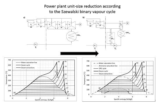
1. Introduction
In the 1960s, Robert Szewalski introduced a binary vapor cycle consisting of a supercritical steam cycle and an organic Rankine cycle (ORC) coupled in a hierarchical energy system. The purpose of this idea was to facilitate the design of power units producing a few gigawatts of power.
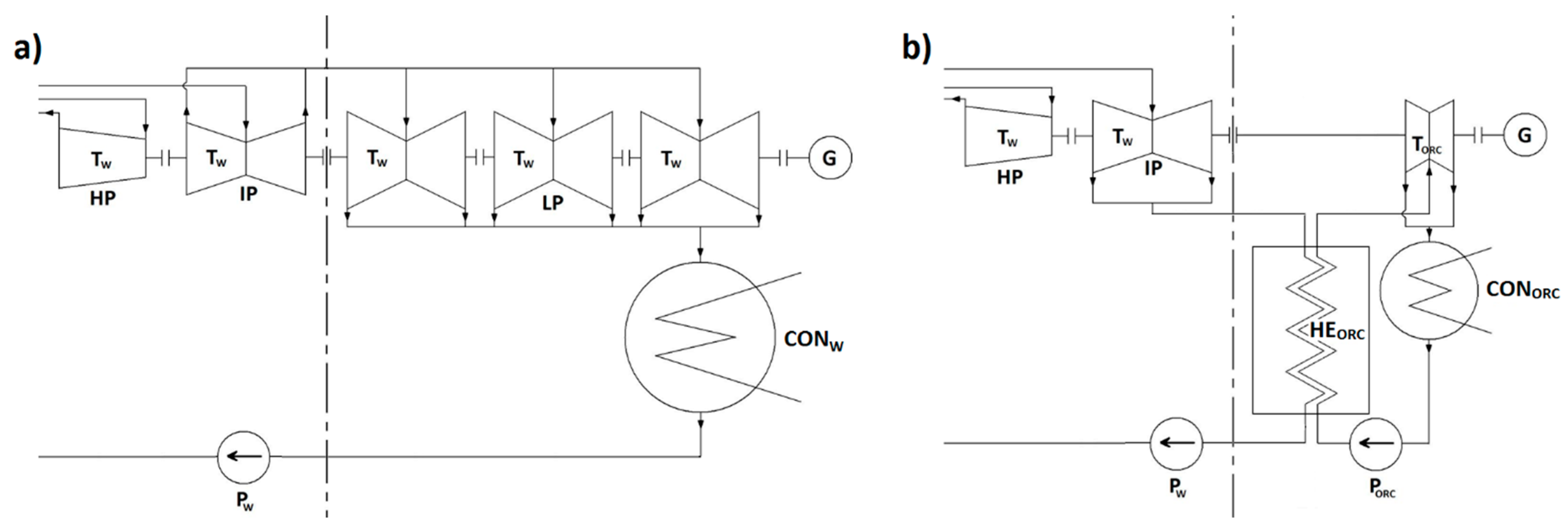
Here, we present the generally accepted terms and common parts of the binary cycle and ORC. We next discuss the primary differences between typical binary cycles and the Szewalski cycle, and we explain the Szewalski cycle in particular. We note that the entire system consists of a traditional steam cycle and the ORC. The Szewalski binary vapor cycle [1,2] uses steam as a working fluid in the high-temperature part of the cycle; another fluid—an organic working fluid with a low specific volume—is used as a working substance that takes the place of conventional steam over a range of temperatures represented by low-pressure (LP) steam expansion (Figure 1).
Figure 1.
Scheme of the Szewalski binary vapor concept cycle (b) compared with the conventional supercritical steam cycle (a). LP—low-, IP—intermediate-, and HP—high-pressure part of the steam turbine. HEORC—regenerative heat exchangers, PW—water pump, G—generator, CONW—condenser of water steam, TW—steam turbine, TORC—turbine of low-boiling point fluid, PORC—pump of low-boiling point fluid, CONORC—condenser of vapor of low-boiling point fluid.

The binary vapor cycle is a thermodynamic cycle that converts thermal into mechanical energy. It is composed of two sub-cycles that employ two different working fluids. The most common applications include serial coupling of sub-cycles, but a parallel configuration is also possible [3,4]. Binary sets have been well known since the beginning of the 20th century. A mercury-steam cycle was introduced to improve the steam cycle efficiency by increasing the working fluid’s temperature without increasing its pressure [1,2], which is consistent with the theory of the Carnot heat engine efficiency [5]. The development of material science and production technology has led to complex and expensive binary sets being replaced by steam sets with live steam parameters of 550 °C and 15 MPa or higher [6,7].
However, the importance of the binary cycle increases in the low-temperature range—for example in geothermal power engineering. In geothermal power plants, the first working fluid was geothermal water or steam that only heated the second fluid (i.e., pure steam in a closed steam turbine cycle) [8]. The goal of this methodology was to separate the turbines from water containing mineral inclusions. However, for the last three decades, geothermal power plants have been intensively developing low-boiling point fluids. ORCs can use low-temperature geothermal heat sources because of their low operating temperatures. Hence, they attain a low thermodynamic efficiency typically in the range of 0.08–0.12 [8,9].
The low thermodynamic efficiency of ORCs does not mean that they cannot be effectively used to generate electricity. ORCs usually attain high exergetic efficiencies that are comparable to the efficiency of steam cycles, without taking boilers into account. Secondly, due to a cascade application it is possible to couple an ORC with a conventional Rankine cycle or to another ORC in very efficient applications by optimally matching the cycle thermodynamic parameters to the heat source and sink. In this case, the condenser of one sub-cycle is simultaneously an evaporator of the next one [3,8,10,11]. More so, the application of low-boiling point fluids in energy cycles is associated with advantages other than the utilization of low-temperature heat sources [11]. One of these advantages is employed in the Szewalski binary vapor cycle.
Studies and a patent by Szewalski [1,2] operate on a specific assumption, which is presented below. According to Szewalski, a supercritical steam cycle is preferred due to its high efficiency in the primary part of the cycle. In the second part of the cycle, the ORC provides a working fluid with a low specific volume. The objective of this concept is to significantly reduce the LP turbine sizes and hence make it possible to increase the output power attainable by a single turbine unit [1,2]. This process leads to an increased gross efficiency of the power plant gross and a decreased specific investment and maintenance costs [1,2,12].
The low specific volume of the LP turbine outlet steam in condensing power plants leads to an increase in the demand for materials. The cylinder of the LP turbine, in units of approximately 600 MWe of output power and above, is typically divided into three parallel casings in which the last-stage blades are limited to approximately one meter [7]. Moreover, because steam starts to condensate at the last stages of the LP turbine, very expensive materials are required to prevent corrosion and erosion and to withstand the large mechanical stresses. For instance, the LP part of a conventional turbine-unit with about 600 MWe with three double-flow low LP cylinders (casings) has an output of approximately one third of the entire set up; its initial cost is in the order of two thirds of that of the entire unit. If we can decrease the cost of this part that now includes the cold vapor turbine and the heat exchanger to one half of the cost of the conventional design, then the cost of the entire unit will be only two thirds of the previous cost. This decrease is significant given that the economic considerations are tied to real technical progress [1]. A scheme of the size reduction is presented in Figure 1.
The most recent analysis of thermodynamic and operational parameters of the Szewalski binary vapor cycle was performed by Ziółkowski et al. [7]. This analysis was carried out using accessible numerical Computational Flow Mechanics (CFM) codes via step-by-step modeling of separate apparatuses. In the Szewalski binary vapor cycle, we considered four potential working fluids (propane, isobutene, ethanol and ammonia) to obtain the highest output and a First Law efficiency of the cycle.
Another supercritical steam cycle that utilizes an ORC cycle has been analyzed in the literature [13,14]. The objective of these studies was to analyze the thermodynamic and operational parameters of a supercritical power plant given reference conditions; this research also focused on the introduction of a hybrid system incorporating an ORC. In an ORC, the upper heat source is a stream of hot water from the system of heat recovery with a temperature of 90 °C, which is additionally aided by heat from steam bleeds of the LP steam turbine. Ziółkowski et al., conducted a thermodynamic analysis of the supercritical plant with and without incorporation of the ORC using CFM numerical codes. Four fluids (propane, isobutane, pentane and ethanol) were investigated in [13], and six working fluids (propane, isobutane, pentane, ethanol, R236ea and R245fa) were investigated in [14]. In the course of the calculations, it was determined that the unit power increased and that a First Law efficiency was attained for the reference case and the case with the ORC.
An analysis of literature results [7,13,14,15,16,17,18,19,20,21,22,23,24,25,26,27,28,29,30,31,32,33,34] pertaining to exergy confirms that good resolution is to perform the exergy loss analysis in the Szewalski cycle.
Exergy analysis is an important tool for the optimization of complex thermodynamic processes because energy balance alone does not include entropy generation and therefore energy quality degradation. For technical and economic reasons, the quality of energy is closely related to investment and maintenance costs [16,17,18]. It should be noted that a First Law analysis is not only incomplete but also misleading because it distorts the real resource consumption quantifiers and overestimates low-exergy (high-entropy) fluxes [17].
A good example of an exergy analysis of a power cycle is [19], in which the authors present an original and rapid method for heat recovery steam generator (HRSG) exergetic optimization. The main aim of the analysis is to maximize exergy transfer to the water/steam cycle. The proposed approach fixes the pinch point and the economics by imposing the total heat transfer area of the HRSG. In another study [20], the author proposes reconsidering direct and inverse configurations of Carnot machines, and he presents two examples. The first example is concerned with a “thermofrigo-pump” in which the two utilities are hot and cold thermal exergies due to the difference in the temperature level compared with the ambient temperature. The second example is relative to a “combined heat and power” (CHP) system [20].
It should be noted that due to environmental-impact considerations and energy-conversion efficiency, the renewal and development of heat pumps and CHP systems has been increasing from large- to micro-scale systems (μCHP) for industrial, building applications and even photovoltaic/thermal (PV/T) configurations or fuel cell CHP systems [17,21,22,23,24,25,26,27,28,29,30,31,32]. Energy and exergy analyses have been conducted by many authors, for example: (1) a combined heat and power system by Feidt & Costea [28]; (2) a novel hybrid solar heating, cooling and power generation system for remote areas by Zhai et al. [22]; (3) a combined molten carbonate fuel cell-gas turbine system by El-Emam & Dincer [25]; (4) a comparison of Proton Exchange Membrane Fuel Cell and Solid Oxide Fuel Cell-based μCHP systems by Barelli et al. [27]. Additionally, exergy analyses of poly-generation systems for sustainable building applications were conducted by Bingöl et al. [26]. Nieminen & Dincer [24] compared gasoline and hydrogen fuelled internal combustion engines using exergy analyses. A review of exergo-economic analysis and optimization of combined heat and power production was performed by Abusoglu & Kanoglu [23].
An exergy analysis offers useful insights into the correct assessment of the process itself: It identifies and quantifies the sources of irreversibility and allows for an immediate comparison of different process structures. Furthermore, such an analysis provides a clear indication for the resource-to-end-use matching, thus enabling better resource allocation. Its inability to account for externalities limits its usefulness in a broader context, however. Additionally, extended exergy analysis overcomes this latter limitation and provides a complete picture of how the process interacts with the biosphere and with the societal environment [31].
According to Szargut’s proposal [33], exergy is an adequate measure of the quality of natural resources. A complete example concerning the analysis of thermo-ecological cost has been presented in [32]. These authors focus on an ecological analysis of coal injection as auxiliary fuel to the Tuyere zone of a blast furnace. Connections with coalmines, coke-oven batteries and power plants have been considered. The summary of Szargut’s investigations on this subject has been presented in [33]. In a recent work, Ziębik and Gładysz [34] presented an algorithm for calculating the thermo-ecological costs of an integrated oxy-fuel combustion power plant based on an “input-output” model of direct energy and material consumption and also on the application of an “input-output” approach for the construction of a mathematical model of the thermo-ecological costs of such a power plant. In order to construct this model, the authors assumed that interconnections between the analyzed integrated oxy-fuel combustion power plant and domestic economy were rather weak, which permitted them to establish indices of thermo-ecological costs concerning fuels, raw materials and semi-products on the basis of a priori knowledge [34]. However, the thermo-ecological optimization of a solar collector was also established [30].
Exergy is a suitable measure of differences in the environment. Various authors have examined the concept of sustainability in relation to exergy flows on Earth. Exergy is applied to emissions into the environment using case studies in order to describe and evaluate its values and limitations as an ecological indicator. Exergy has also been considered to be a useful ecological indicator according to the literature [35].
Exergy accounting has been successfully used for diagnosing energy systems and for accounting for the Earth’s exergy resources. Both applications rely on the concept of exergetic cost. This concept attempts to measure the amount of exergy resources necessary to produce any effect. The process of cost formation becomes essential to understanding and evaluating exergy costs and the degradation process of resources feeding a system. Cost, irreversibility and causation become deeply interrelated, and an Aristotelic analogy between cause and thermo-economic concepts is highlighted [36].
Besides applications to “systems engineering”, another area in which exergy analysis is of importance is the allocation of funding for research and development, irrespective of whether the funding is corporate, entrepreneurial or governmental. Furthermore, exergy analysis can be used for establishing policies [17,37].
From an economical point of view, the construction of powerful steam turbine sets is desirable. First of all, due to the increase in machinery output power (steam boilers, feed water pumps, turbines, even the size of power plant halls), specific investment costs are decreasing. Secondly, machinery efficiency is always higher for large applications [1,2,6,7]. Moreover, maintenance costs such as the number of power plant staff, logistics, renovations, diagnostics, etc., are also relatively lower for larger applications.
Here, we present a Szewalski binary vapor cycle exergy loss analysis. However, in order to present the issue correctly our analysis is based on meaningful values using power plant data [7,13,14]. Our methodology consists of the following steps:
- -
- The creation of a steam cycle mathematical model convergent with a supercritical power plant cycle;
- -
- The choice of optimal parameters for the “cut-off” LP steam turbine;
- -
- The optimization of the ORC thermodynamic parameters;
- -
- The selection of the low-boiling point working fluid for the ORC installation;
- -
- A comparison of exergy losses in the reference cycle and the Szewalski cycle using collected data;
- -
- A summary and conclusion.
2. Referent Model of a Supercritical Steam Cycle
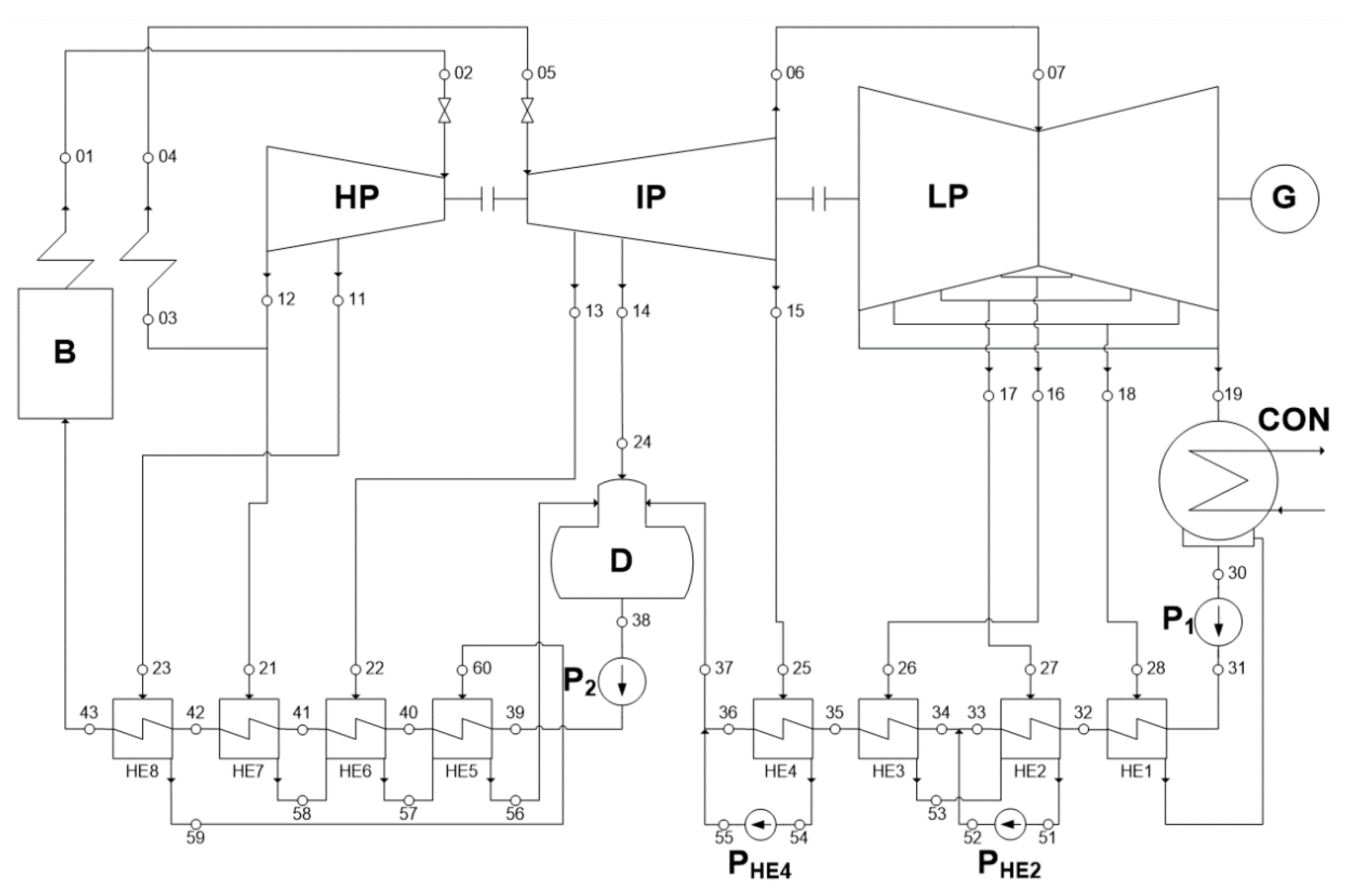
Our analysis of the exergy losses in a binary vapor cycle is based on a CFM model of supercritical steam power, which we refer to as a reference model. The thermodynamic cycle consists of a steam boiler (B) with a steam superheater and re-heater, a three-cylinder (casing) steam turbine (HP, IP, SP) with an electric generator (G), a condenser (CON) and a feed water regeneration system (HE1–HE8) with a deaerator (D).
The thermodynamic parameters of the reference model have been validated using literature data [7,14]. The most significant difference between the reference model and literature data is a steam turbine output power lower by about 510 kW, i.e., 899,490 kW for the reference model and 900,000 kW for a real cycle. A list of the most important cycle parameters and assumptions can be found in the appendix (Supplementary data—Table S1). A full list of the reference model thermodynamic parameters, according to Figure 2, is presented in the appendix (Supplementary data—Table S2). A correct and convergent mathematical model was the basis for our entire analysis.
Figure 2.
Thermodynamic scheme of the supercritical steam power plant-reference model: B—steam boiler with superheater, HP—high-pressure steam turbine, IP—intermediate-pressure steam turbine, LP—LP steam turbine, P—water pumps, CON—condenser, D—deaerator, G—electric generator, HE—regeneration heat exchangers.

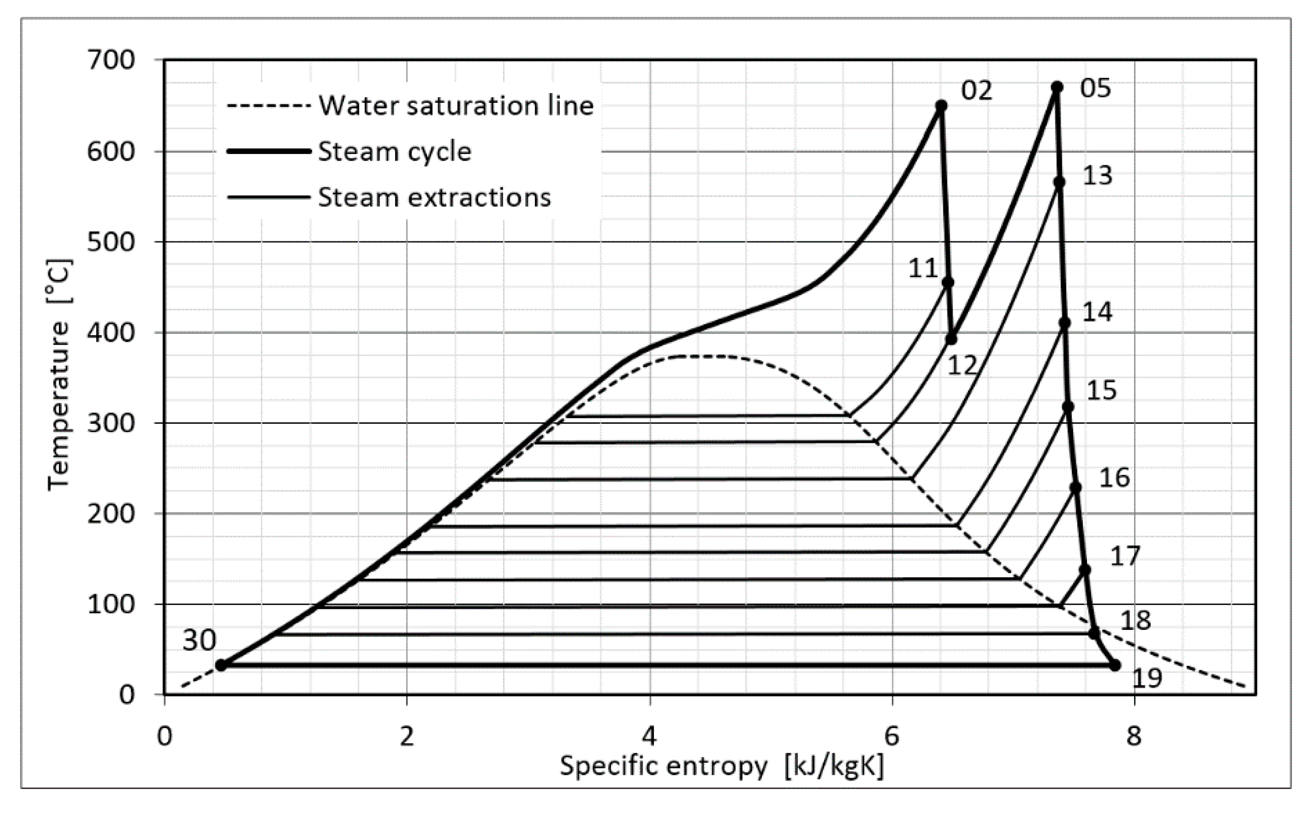
In order to more clearly show the heat transfer and steam expansion phenomena occurring in the reference model devices, a temperature-specific entropy diagram is shown in Figure 3. The characteristic points of the thermodynamic cycle are labeled the same as in Figure 2. Bold lines indicate the main thermodynamic cycle, thin lines indicate steam extractions and their condensation temperatures and dashed line indicates the water saturation line.
Figure 3.
Characteristic thermodynamic points of the reference model represented in a temperature-specific entropy diagram.
Figure 3.
Characteristic thermodynamic points of the reference model represented in a temperature-specific entropy diagram.

The steam expansion from point 18 to 19 occurs with a lower efficiency than in other parts of the turbine for two reasons. The steam turbine reaches a lower isentropic efficiency during expansion in the range of wet steam. This phenomenon is complex, but, according to Baumann [38], we can simplify the situation and assume that only the gas fraction in the wet steam flow expands and that the liquid fraction is responsible for the flow losses. More accurate explanations, according to Bakhtar et al., and Gyarmathy and Lesch [39,40], involve local subcooling of the steam around the condensation germ. Moreover, the last turbine stage in condensing power plant is designed with some modifications in order to provide a safe working range of wet stem expansion, particularly under partial loads. Therefore, those improvements decrease the efficiency of the design point [38]. Hence the next step is the choice of the optimal parameters for the “cut-off” LP steam turbine.
3. The Szewalski Binary Vapor Cycle
3.1. The Optimal Point of “Cut-off” LP Steam Turbine
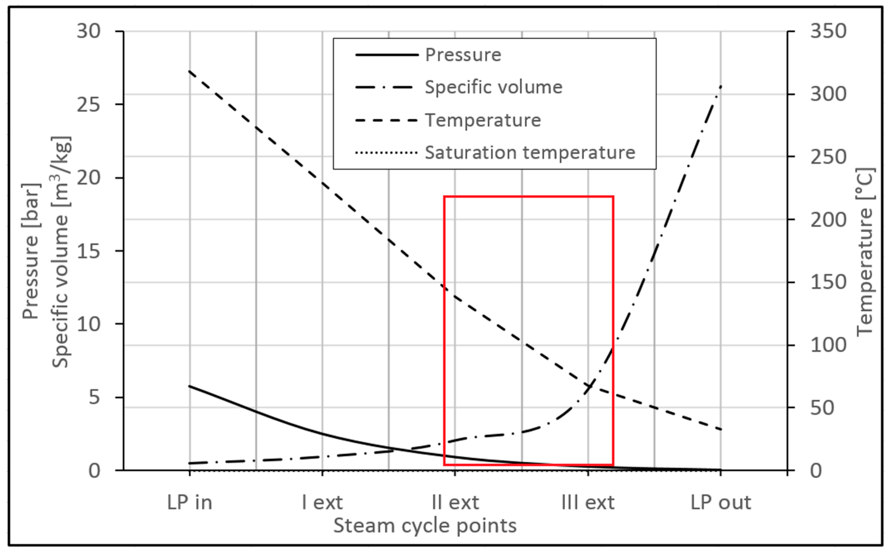
In order to attain the main objectives of the Szewalski cycle, it is necessary to determine the optimal “external” parameters for the ORC installation. To this end, we have analyzed the objective LP turbine in detail. The thermodynamic parameters of steam at the inlet, outlet and steam extractions of the turbine are presented in a diagram of pressure, specific volume and temperature vs. the steam cycle points in Figure 4.
At the inlet to the LP turbine (point 07), the steam is under a pressure of 5.78 bar and is at a temperature of 318 °C. High pressures results in a low specific volume of approximately 0.47 m3/kg. During expansion of the steam in the LP turbine, the pressure and temperature decrease, and the specific volume of the steam increases to values exceeding 25 m3/kg, which means that in an LP turbine the specific volume increases by a factor of over 50. The dimensions of the last stages and the outflow of the turbine result in technical problems that increase the initial costs. Moreover, the high specific volume of the condensation necessitates a large condenser. Under a high vacuum, it is impossible to maintain the seal of the condenser. For this reason, powerful vacuum systems are needed for large condensers.
Figure 4.
A diagram of pressure, specific volume and temperature vs. steam cycle points for an LP steam turbine in the reference model. LP in—LP turbine inlet, point 07 in Figure 2; I ext—first steam extraction in the LP casing; point 16 in Figure 2; II ext—second steam extraction in the LP casing; point 17 in Figure 2; III ext—third steam extraction in the LP casing point 18 in Figure 2; LP out—outlet from the LP turbine.

The optimal point of “cut-off” of the LP turbine, taking into account the dimensions of the turbine and the steam properties, is between the second and third steam extractions (points 17 and 18 referring to the nomenclature of Figure 2 and Figure 3). Besides the dimension criteria, it is also important to consider “external” parameters for the ORC installation. According to the literature [41,42], ORC systems can be effectively operated at a range of temperatures, i.e., 65–140 °C. Other positive results of a “cut-off” in this range of steam parameters include:
- -
- The prevention of steam condensation in the steam turbine, which is associated with corrosion and erosion in the last turbine stages. Furthermore, the last stages of the new LP turbine are shorter and can be made of cheaper materials;
- -
- A less powerful vacuum system in the steam condenser-ORC heat exchanger because the steam condensation occurs at less than 0.25–1 bar of pressure.
For the reasons noted above, further considerations will be based on the steam parameters from points 17 and 18 (Supplementary data—Table S2) extended to the steam condensation temperature in the range of 45–105 °C. As the chosen thermodynamic cycle was adapted to the binary cascade, the majority of the model parameters were not changed. During data collection for different cycle configurations, the thermodynamic and flow parameters up to point 07 (at the LP turbine inlet) and from point 34 (before heat exchanger No. 3) (see the thermodynamic scheme shown in Figure 2) were always constant and the same as for the reference model. A scheme of the Szewalski cycle in the case of a “cut-off” of the LP turbine under the parameters of point No 18 (III ext—third steam extraction) is presented in Figure 5.
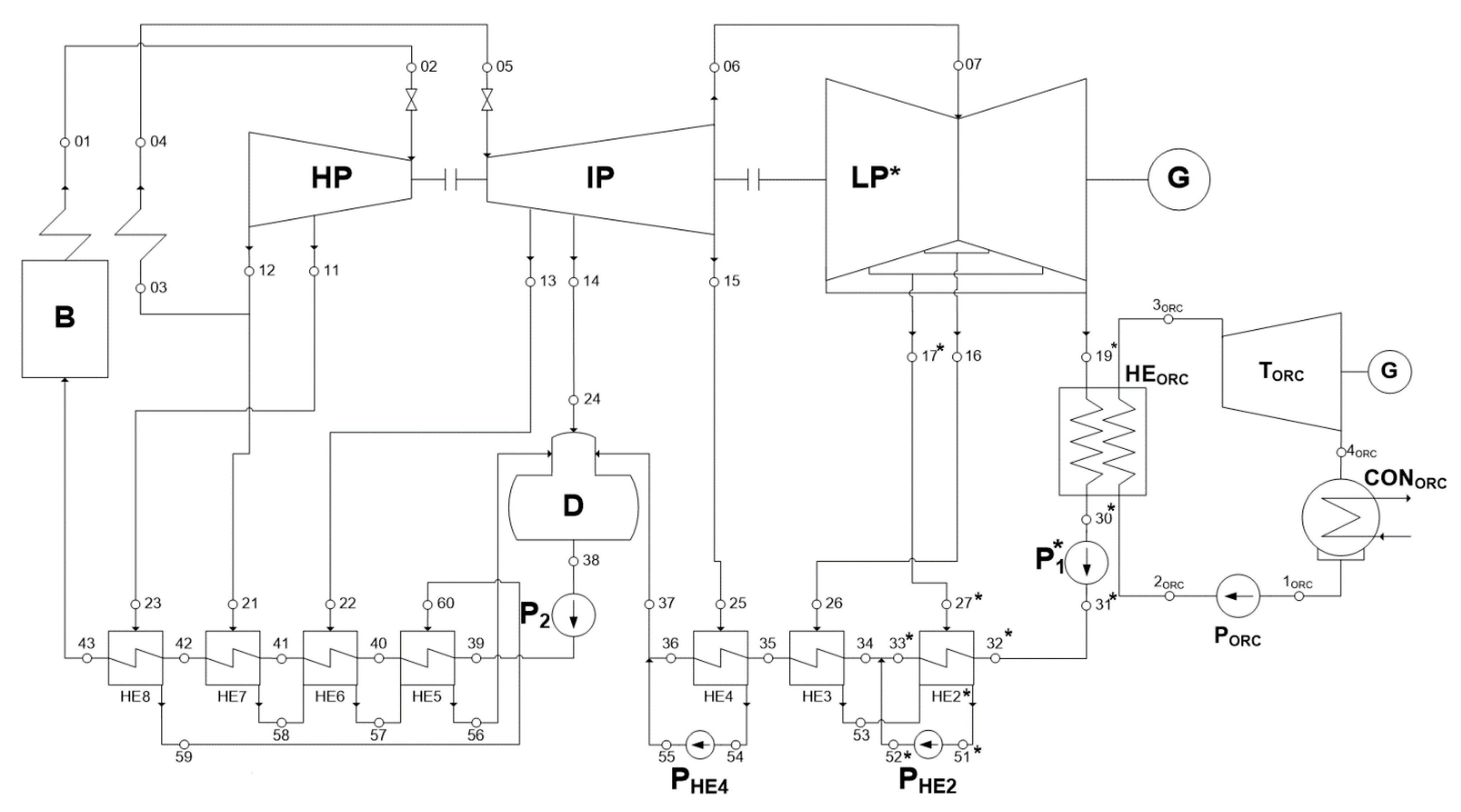
Figure 5.
Thermodynamic scheme of the Szewalski binary vapor cycle: B—steam boiler with superheater, HP—high-pressure steam turbine, IP—intermediate-pressure steam turbine, LP—LP steam turbine, P—water pumps, CON—condenser, D—deaerator, G—electric generator, HE—regeneration heat exchangers; the subscript “ORC” refers to the ORC cycle devices.

In the proposed configuration, heat exchanger No 1 (HE1 in Figure 2) has been removed, and the steam parameters at the outflow of the LP* turbine in point 19* are equal to those at point 18 in the reference cycle. The steam condenser has turned into the ORC heat exchanger, the LP steam turbine has been divided into a new, smaller LP* steam turbine and the ORC turbine (TORC). The ORC condenser (CONORC) has taken on the role of the steam condenser. The ORC pump (PORC) is an added device with no counterpart in the reference cycle. The next steps are the optimization of the ORC part of the hierarchical cycle and the selection of the working fluid.
3.2. The Optimization of the ORC Part of the Hierarchical Cycle
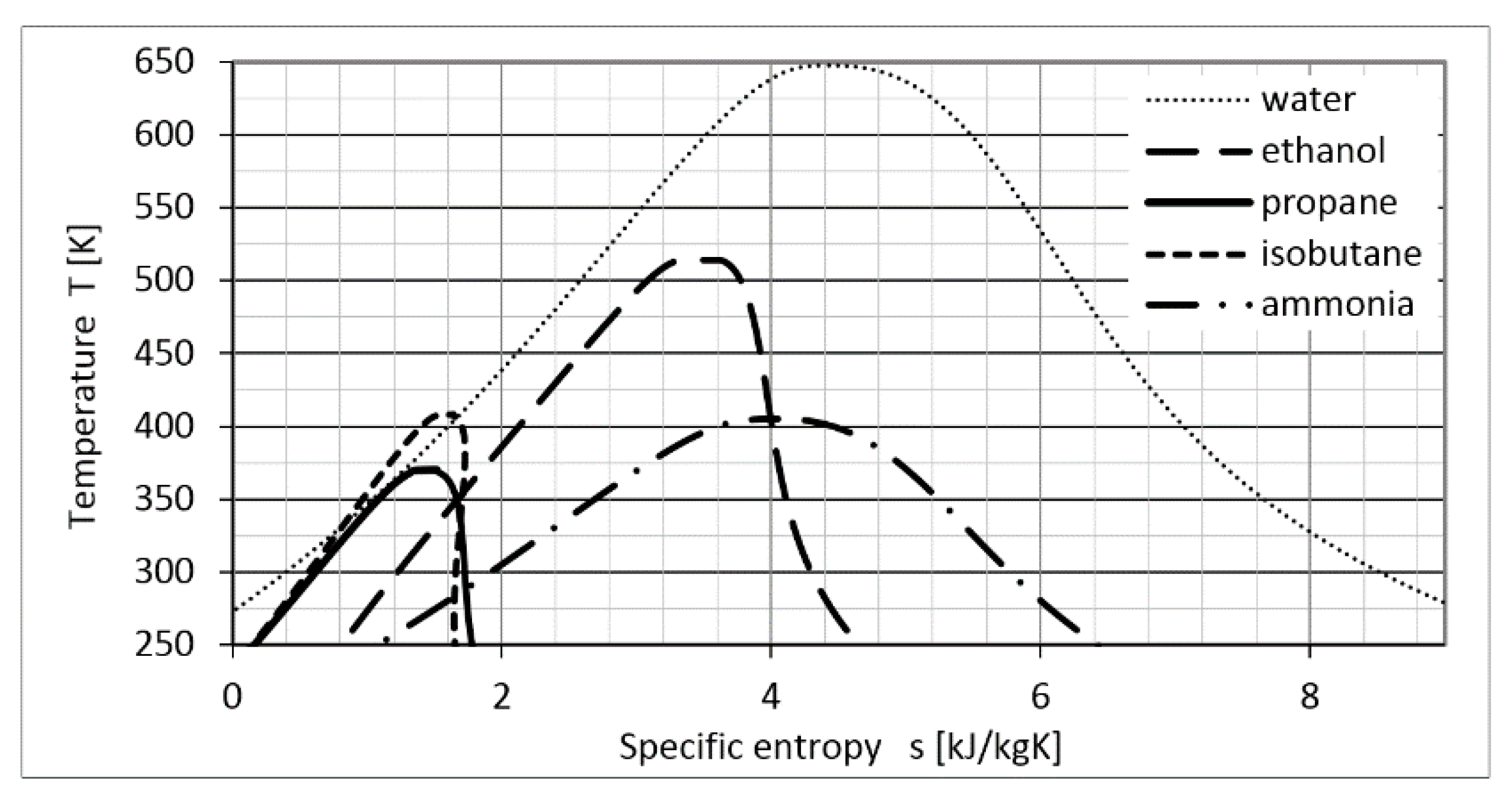
The ORC installation has been designed to be the simplest and therefore also the smallest and the cheapest cycle; it lacks a vapor superheater and regeneration heat exchanger between the ORC turbine and condenser. The Szewalski binary vapor cycle has been tested using four low-boiling point fluids: ethanol, ammonia, propane and isobutane. The fluids were chosen based on literature data [41,42] as being the most suitable for this temperature range. In Figure 6, we show the saturation lines of the chosen fluids relative to a water saturation line in a temperature-specific entropy diagram.
Figure 6.
Saturation lines of the chosen fluids and water in a temperature-specific entropy diagram.
Figure 6.
Saturation lines of the chosen fluids and water in a temperature-specific entropy diagram.

In addition to many parameters such as saturation pressure, specific entropy or specific volume for set thermodynamic conditions, low-boiling point fluids have a parameter that can be used to divide them into three groups: wet fluids, isentropic fluids and dry fluids. This parameter is determined by the vapor saturation curve. If the fluid is dry, then after isentropic expansion from a saturated vapor it will be superheated; these fluids do not need superheating. However, in order to increase the cycle efficiency it is necessary to use a regeneration heat exchanger between the turbine outflow and the condenser. However, even such a device cannot produce wet or saturated steam at the condenser inflow because the main feed pump will always increase the working fluid temperature during pumping. Moreover, to ensure small dimensions of the heat exchanger it is necessary to set a pinch point, which refers to the lowest temperature difference between the evaporating fluid and the heating media [41,42]. In this case, we assumed a pinch point of 5 K.
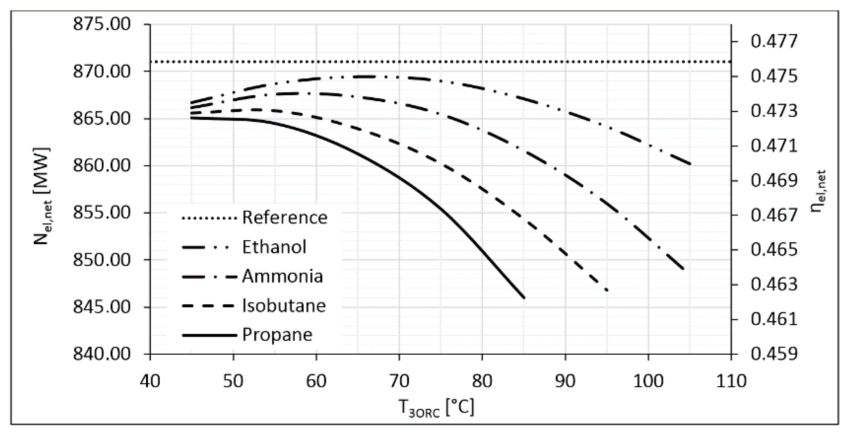
In the case of an isentropic fluid, isentropic expansion from the saturated vapor proceeds along the saturation line and ends at the point of a saturated vapor. A wet fluid acts in the same way as steam: After isentropic expansion from a saturated vapor, the expansion ends in a range of wet fluids. If the working fluid is “wet”, as in the case of water or ammonia, it is preferable to superheat the vapor [41,42]. However, in our preliminary calculations, the same cycle (presented in Figure 5) was used. The results of the preliminary calculation in a diagram of cycle electric net power Nel,net—cycle electric net efficiency ηel,net vs. ORC turbine outlet temperature T3ORC are presented in Figure 7.
The dotted line in Figure 7 refers to the reference cycle electric net power and electric net efficiency, and the curves of the selected fluids refer to those parameters that are due to the different temperatures of the working fluid at the ORC turbine inlet (point 3ORC in Figure 5). The temperature of the steam condensation is 5 K higher, so it is in the range of 50–110 °C. The electric net power Equation (1) and electric net efficiency Equation (2) can be defined as:
where Nel,net is the cycle electric net power, Nel is the electric generator output power, NP is the pump power demand, ηel,net is the electric net efficiency, is the stream of fuel chemical energy, i = 1,2,…,n is the number of pumps.
Figure 7.
Results of the preliminary calculation of the tested fluids in a diagram of cycle electric net power Nel,net and cycle electric net efficiency ηel,net vs. ORC turbine outlet temperature T3ORC.
Figure 7.
Results of the preliminary calculation of the tested fluids in a diagram of cycle electric net power Nel,net and cycle electric net efficiency ηel,net vs. ORC turbine outlet temperature T3ORC.

Preliminary calculations reveal that the highest electric net power and efficiency are achieved for ethanol for a vapor temperature at the inlet to the turbine in the range of 65–70 °C. The second most efficient fluid is ammonia for a temperature of 55–65 °C. Isobutane and propane exhibited the lowest efficiencies. Isobutane vapor at the outlet of the turbine was still a superheated vapor, but the temperature was approximately 10 K above the condensation temperature. Therefore, there was no incentive or technical possibility to use the regeneration heat exchanger.
3.3. Selecting the Low-Boiling Point Working Fluid for the ORC Installation
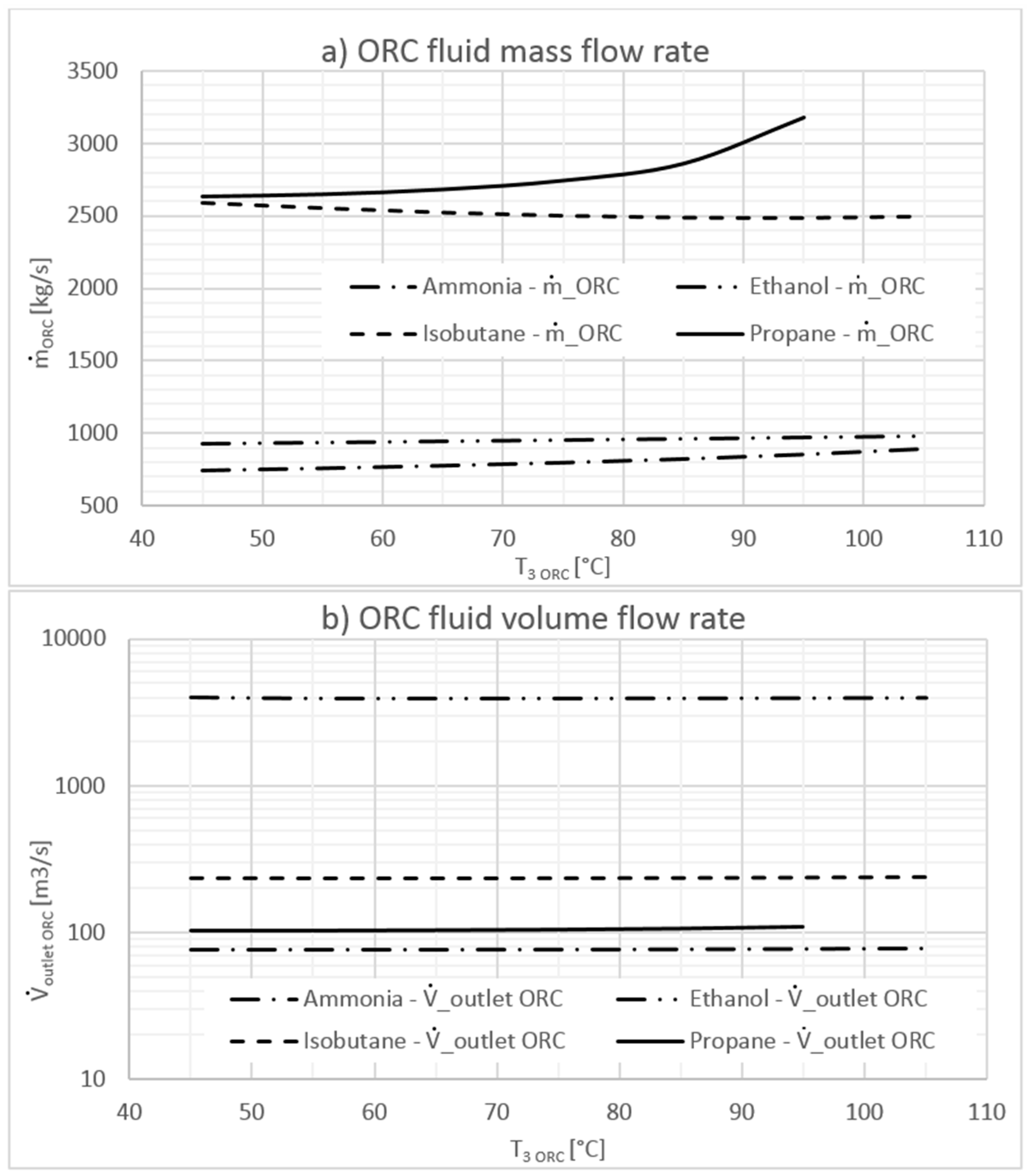
The cycle efficiency was, however, not the primary parameter that we focused on during the preliminary design of the Szewalski cycle. Our main aim was to decrease the size of the LP steam turbine to make it possible to increase the live steam mass flow rate and therefore increase the output power of the unit without additional parallel LP cylinders. A detailed analysis of the ORC fluid mass flow rate and volume flow rate at the ORC turbine outflow for different values of temperature at the turbine inlet (T3ORC) are presented in Figure 8.
We only tested propane up to a temperature of 95 °C because its critical point occurs at approximately 97 °C. Isobutane was the only fluid whose mass flow rate decreased with increasing steam condensation temperature. This finding was due to the fact that the heat consumption during evaporation decreased slightly due to the increase in heat needed for preheating to increase the values of the working fluid pressure. This situation can be observed in the saturation curves in Figure 6. Ammonia had the smallest mass and volume flow rate over the entire tested temperature range. The ethanol mass flow rate was slightly higher, but its volume flow rate was a few thousand times higher (a logarithmic scale is shown in Figure 8).
Figure 8.
ORC fluid: (a) mass flow rate; (b) volume flow rate at the ORC turbine outflow vs. temperature difference between the turbine inlet and T3ORC.
Figure 8.
ORC fluid: (a) mass flow rate; (b) volume flow rate at the ORC turbine outflow vs. temperature difference between the turbine inlet and T3ORC.

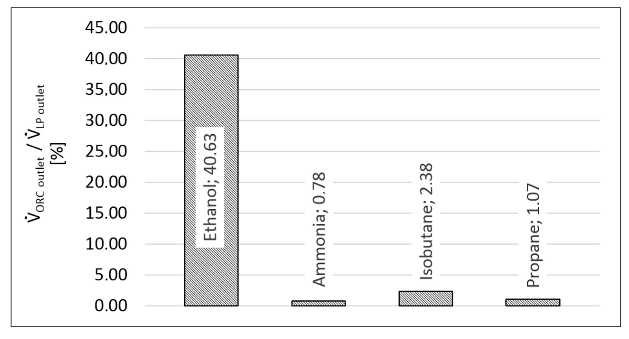
To better visualize the possibility of a volume flow rate decrease, which leads to a decrease in the turbine exhaust area and therefore limits the length of the last-stage turbine blades, the ORC turbine outflow volume rate was compared with the LP steam turbine outflow volume rate of the reference model. The results are presented in Figure 9.
Figure 9.
ORC turbine outflow stream volume as a fraction of the reference model LP steam turbine outflow stream volume for the tested fluids assuming their optimal cycle parameters.
Figure 9.
ORC turbine outflow stream volume as a fraction of the reference model LP steam turbine outflow stream volume for the tested fluids assuming their optimal cycle parameters.

Using the most efficient fluid, ethanol, leads to a decrease in the volume flow rate of about 60%; for ammonia, the decrease reached 99%. This result is possible because the specific volume of vapor at the ORC turbine outlet (point 4ORC in Figure 5) reached approximately 0.09 m3/kg compared with 26.21 m3/kg in the case of steam in the reference model. The saturation pressure of ammonia at 32 °C is equal to 12.6 bar, and the dryness fraction during expansion drops to 0.93, which is the same value as for steam in the reference cycle. It should be noted that the exhaust area is proportional to the volume flow, but the flow channel diameter to volume flow follows a square-root dependence. Therefore, given a one hundred-times decreased volume flow rate due to an assumption of constant velocity leads to a flow channel diameter reduced in length by a factor of 10. Additionally, turbine blade length is a complex function of flow parameters, geometry and shaft rotation speed.
Ammonia as a working fluid in the ORC installation yielded nearly the highest cycle efficiency and the largest decrease in the size of the unit. For these reasons, all later analyses were based on the Szewalski binary vapor cycle model with ammonia. We compared the results of the Szewalski cycle calculations with the reference model data. The main parameters were the electric generator power, the pump demand, the electric output power and the cycle’s net efficiency. Explanations in the form of equations and parameters are presented in Table 1.

| Parameter | Symbol | Units | Reference Model | Szewalski Model (Ammonia) |
|---|---|---|---|---|
| Electric generator power | Nel | kW | 899,490 | 899,226 |
| Pump demand | kW | 28,874 | 31,791 | |
| Electric output power | kW | 871,126 | 867,434 | |
| Cycle electric net efficiency | % | 47.58 | 47.39 | |
| LP* turbine exhaust channel diameter relative to the LP turbine diameter | % | - | 40 | |
| TORC turbine exhaust channel diameter relative to the LP turbine diameter | % | - | 10 | |
| Mass stream of water | kg/s | 619 | ||
| Mass stream of ammonia | kg/s | - | 860 | |
| Live steam/vapor temperature | t02/T3ORC | °C | 650/- | 650/65 |
| Live steam/vapor pressure | p02/p3ORC | bar | 300/- | 300/29.40 |
| Steam/vapor condensation temperature | t30/T1ORC | °C | 32/- | 70/32 |
| Steam/vapor condensation pressure | p30/p1ORC | bar | 0.05 | 0.31/12.6 |
The results in Table 1 are presented for ammonia, however a comparison of the calculation results for the other tested fluids revealed that the pump demand increased the most for ethanol (by more than 7 MW). For ammonia the pump power demand was relatively high due to the high pressure ratio between the set saturation and the condensation temperature. However, the pump demand had no influence on the output power of the turbines. Therefore, additional losses in the proposed cycle only slightly decreased the turbine output power.
The reference model was altered by the replacement of the LP steam turbine with a new smaller one with an additional ORC turbine (TORC). The LP turbine efficiency was divided into parts, i.e., 0.80 for the last stage and 0.85 for other stages. As the dimensions of the ORC turbine were significantly reduced with respect to the LP turbine, the outflow to inflow dimension rate was also smaller, and the dryness fraction of the expanded vapor was the same as that for steam. As a result, the ORC turbine can be designed with a higher efficiency. We assumed a value of 0.90 for the ORC turbine internal efficiency. Next, the ORC condenser (CONORC) took on the role of the steam vacuum condenser because in both cycles the operation conditions were the same. The ORC vapor generator (labeled HEORC in Figure 5) was added in the place of the regeneration heat exchangers (depending on the configuration HE1 or HE1 and HE2, as shown in Figure 2). The vapor generator is at the same time also a steam condenser. The advantage of this solution is a small heat exchange surface relative to the conventional steam condenser cooled with water, thanks to higher heat transfer coefficients [1,2,41].
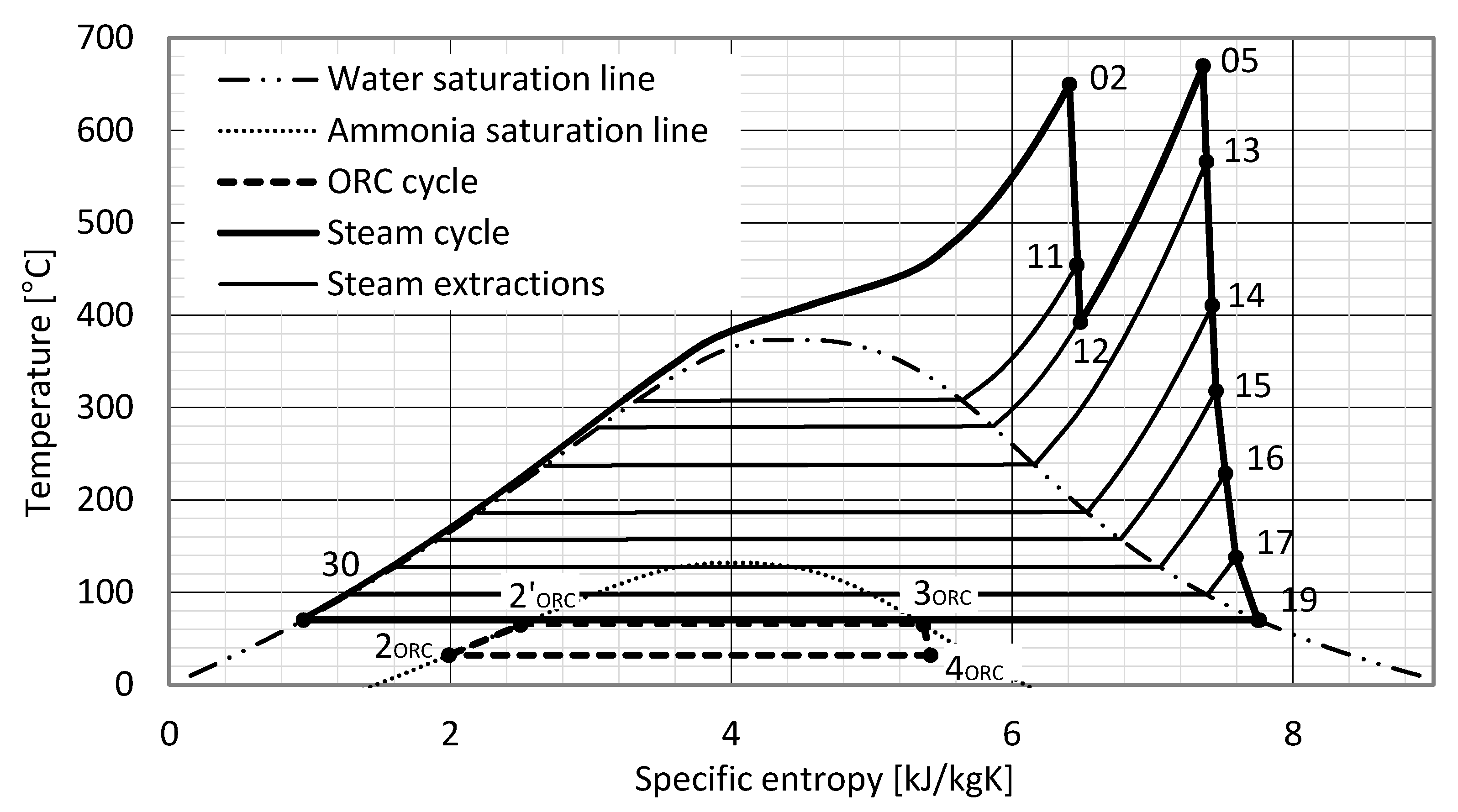
Our proposed Szewalski thermodynamic cycle interpretation in a temperature-specific entropy diagram is presented in Figure 10.
Figure 10.
Thermodynamic interpretation of the Szewalski cycle in a temperature-specific entropy diagram assuming ammonia as the working fluid.
Figure 10.
Thermodynamic interpretation of the Szewalski cycle in a temperature-specific entropy diagram assuming ammonia as the working fluid.

This visualization helps to understand the thermodynamic modifications to the steam cycle during modernization into a binary vapor cycle. Due to our chosen thermodynamic parameters, steam condensation occurs at higher temperatures, and the expansion of the ammonia in the ORC turbine takes the place of steam expansion in the LP turbine. The new LP* steam turbine is smaller due to a smaller specific volume flow at the outflow of the turbine. Moreover, the expansion in the turbine is “shorter” and occurs between points 15 and 19*. Given the two-fold lower specific entropy of ammonia, as shown in Figure 10, the mass flow rate must be almost two times higher than the mass flow rate of condensing water. Entropy balance shows that due to our chosen parameters, the increase in entropy (generation of entropy) is small. However, to optimize the energy conversion efficiency of the Szewalski cycle, we employed exergy analyses.
4. Exergy Balance
To conduct a reliable analysis of a thermodynamic cycle, particularly a complex hierarchical cycle, exergy analysis in addition to thermodynamic analysis is recommended [43,44,45]. Exergy analysis yields a value of efficiency related to the “available energy” that can be converted into work [45,46]. The main feature of exergy is the usage of the thermodynamic temperature, which involves entropy generation. In this case, the ideal Carnot cycle always reaches 100% efficiency, and it shows if the analyzed cycle is closer to or further from the Carnot cycle efficiency [43,44]. Moreover, due to the analysis of exergy losses in the cycle it is possible to undertake proper optimization steps in selected devices to improve technical processes. Exergy analysis is particularly helpful for heat-transfer processes.
To begin the exergy analysis, we describe the exergy stream according to [44] as a sum of a usable part of the internal and external streams of energy:
where describe the potential and kinetic streams of energy, respectively, and is a thermal exergy stream consisting of two elements:
The e element describes the stream of physical exergy, which includes pressure and thermal exergy stream differences between the substance thermodynamic state and ambient parameters. The parameter describes the chemical energy of the substance assuming ambient temperature and pressure.
Narrowing down our considerations to fluid-flow machinery with adiabatic insulation from the environment, we can assume that the maximal technical work of the machinery is equal to the thermal exergy decrease of the thermodynamic fluid, which can be written as:
where are the inlet and outlet enthalpy streams of the process, respectively, and is the amount of useless heat exchanged with the environment.
According to the entropy definition from the Second Law of thermodynamics, the thermal exergy decrease can be described as:
where is the ambient temperature and are the inlet and outlet entropy streams, respectively.
However, if the chemical energy conversion of fuel in the combustion chamber, boiler or fuel cell is taken into consideration, Equation (6) must be applied to the stream of physical energy and then Equation (4) becomes:
The procedure for evaluating the chemical exergy depends on the type of the reaction and the substrates. A complete procedure for a combustion process is presented in [43,44].
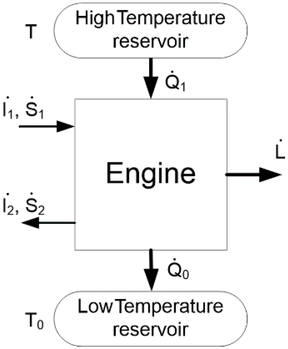
To close the exergy balance of the thermodynamic process, it is necessary to define the exergy losses. To illustrate the balance equations, a model of a thermal engine is presented in Figure 11.
The proposed engine, a binary vapor cycle in this case, using a stream of thermal energy yields a stream of mechanical work and exhales a stream of worthless thermal energy . Additionally, coolant with an inflow stream enthalpy and entropy is heated to parameters ,
Figure 11.
Model of a thermal engine.

In general, the stream of exergy losses in machinery can be defined using an energy balance equation of real and ideal processes, respectively:
Using real and ideal processes and the stream of work definition based on Equations (8) and (9), the stream of exergy loss is defined as the difference between ideal process and real process streams of work, or stream of waste energy from real and ideal processes:
According to the Second Law of thermodynamics, the sum of the entropy streams in a system is more than 0, and the stream of entropy generation during a process can be described as:
In the ideal process, the sum of entropy streams equals 0:
By subtracting Equation (11) from Equation (12), we obtain:
Furthermore, by inserting Equation (13) into Equation (10), we can define the stream of exergy losses as the Gouy–Stodola law [43,44]:
To analyze the share of each machine in the cycle relative exergy losses, it is useful to employ the proportion of the exergy losses in the cycle driving exergy as a mass flow rate of the fuel and unit fuel exergy [43,44]:
where is the fuel mass flow rate, bFuel is the specific fuel exergy and is the stream of exergy losses.
For example, the relative exergy losses in a model of a one-cylinder steam turbine and electric generator set ξT-G are given by:
The same losses for a steam condenser are given by:
where is the steam mass flow rate, is the turbine mechanical efficiency, is the electric generator mechanical and electrical efficiency, is the dryness fraction of the turbine outlet steam, is the specific evaporation heat, is the steam absolute temperature, are the steam and condensate specific entropy, respectively, are the steam and condensate specific enthalpy, respectively and are the steam and condensate specific exergy, respectively.
The most general and the simplest formula for the exergetic efficiency refers to the ratio of the driving exergy BD,s of a reversible ideal thermodynamic process to the driving exergy of a real process BD [43,44]:
In Equation (18), one can see that the ideal Carnot cycle attains an exergetic efficiency of 100%, which is why, in general, the exergetic efficiency of thermodynamic cycles can be viewed as a fraction of the Carnot ideal cycle. A more accurate equation depends on the kind of physical process or, in case of the thermodynamic cycle, on the complexity of the cycle. For instance, the gross exergy efficiency of a steam boiler Equation (19) and the exergy efficiency of a pump Equation (20) can be given as:
where is the pump mechanical efficiency, is the pump internal efficiency and is the pumped media mean absolute temperature.
Equation (19) can be used to determine the exergetic efficiency of a heat exchanger by measuring the change of the mass stream and specific exergy of fuel in a heating media mass stream and the specific exergy difference at the inlet and outlet of the heat exchanger. The exergetic efficiency of a more complex model of real machinery or a thermodynamic system can be easily estimated via a balance of losses:
where the index i is the number of machines.
For a simple model of the Clausius–Rankine cycle, the exergy balance is given as follows:
A Comparison of Exergy Losses in Considered Cycles
In the present case in which the ORC installation is added to a supercritical steam cycle, we propose to perform the exergy analyses only for the added devices to investigate their impact on the entire cycle. This line of reasoning for the optimization analysis is used to minimize the costs of implementing the Szewalski idea in a supercritical power plant. Secondly, the steam cycle is already optimized, and changing its parameters is undesirable. The steam cycle parameters were changed between the LP turbine second steam extraction (point 17 in Figure 5) and the regeneration heat exchanger HE2. The results of simplified exergy analyses of the reference cycle machinery and their equivalent machinery in the Szewalski cycle are presented in Table 2.
| Devices | Type Value | Exergy Analysis | ||
|---|---|---|---|---|
| Reference Cycle | Szewalski Cycle | Reference Cycle | Szewalski Cycle | |
| LP | LP* + TORC | 0.02 | 0.02 | |
| CON | CONORC | 0.03 | 0.04 | |
| HE1 | HEORC | <0.01 | <0.01 | |
| 0.71 | 0.89 | |||
| HE2 | HE2* | <0.01 | <0.01 | |
| 87 | 0.84 | |||
| - | PORC | - | <0.01 | |
| - | 0.87 | |||
The values in Table 2 were calculated according to the equation for the exergy balance. The main assumptions, such as fuel exergy for hard coal, condensation exergy, steam exergy, etc were assumed based on the literature data [33]. Further parameters for calculation, such as temperature, mass flow rate, specific enthalpy, etc., are shown in Supplementary data—Table S2.
The exergy analysis reveals that the replacement of one LP steam turbine by a smaller LP* steam turbine and a TORC turbine does not increase the exergy losses because the internal efficiency and enthalpy drops are nearly the same in both cycles. Moreover, the “external” thermodynamic parameters for LP and LP* + TORC are constant. The slight increase in the related exergy losses in the ORC condenser (CONORC), even though the same thermodynamic efficiency is employed in both cycles, is caused by an increase of condensation temperature and the removal of one steam extraction and regeneration steam exchanger. This increase of temperature and the removal lead to an increase of heat injected into the condenser, which causes higher related losses. The next modification concerns the replacement of the regeneration heat exchanger HE1 by the ORC vapor generator (HEORC). In both cycles for the presented thermodynamic configuration these devices have no significant influence on the exergy losses of the cycles. However, if the LP turbine “cut-off” point is selected for higher steam parameters to further reduce the size of the LP turbine, then the exergy efficiency decreases, and the related exergy losses will be more significant.
The device that was not changed was heat exchanger HE2. Its thermodynamic parameters, however, were changed. When the low temperature regeneration system was changed, the role of the heat exchanger HE2* was to compensate the difference in the Szewalski cycle. We assumed that the cycle parameters after the HE2 would be the same for both presented cycles. To demonstrate the subtle changes in the exergy balance of presented cycles, the exergy efficiency . of heat exchangers and ORC pump have been added to Table 2. It should be noted that in both cycles the energy efficiency of the heat exchangers is assumed to be 99.5%. Such a large difference between the energy and exergy efficiency results from entropy generation, which is taken into account in the exergy balance.
A device that has been added to the Szewalski cycle, but has no equivalent in the reference model, is the ORC pump. Through its high internal and exergy efficiency it can have a significant impact on related exergy losses, the net electric cycle output power and the net efficiency. In the configuration of thermodynamic parameters that we present, these losses are very low. However, increasing the pressure ratio in the ORC cycle increases the role of the pump in the balance. This situation occurs when higher thermodynamic parameters of the ORC cycle are adopted. Then, in order to provide a proper temperature for the evaporation of the working fluid, the pressure in the heat exchanger needs to be increased. Superheated ammonia vapor is recommended only in cases in which superheated steam is used to supply the HEORC exchanger to optimize the heat transfer. A different pressure ratio in the ORC installation can also occur for different working fluids. For instance, as shown in Figure 7, the model that we investigated for each low-boiling point fluid generated almost the same amount of electricity at the optimal point. This result occurs because the exergy losses in all devices are minimalized and are almost the same. However, the electric net power is different for each fluid. This difference is caused by the different pressure ratios in the cycle for each low-boiling point fluid, which also accounts for the differing pump power demands. A decreased pressure ratio is recovered for ethanol, ammonia, isobutane and propane, in that order, which is consistent with the diagram shown in Figure 7. Changes in the power demand of the condensate pump, P in Figure 2 and Figure 5, in the analyzed cycles was negligible.
5. Conclusions
Our analysis has revealed that the Szewalski binary vapor cycle has a great potential in the field of reducing the size of power units. Such a reduction can be used particularly for designing units with a large output power, which is desirable for the many technical and economic reasons noted in this manuscript. Unfortunately, the binary cycle is associated with some energy losses and a slight decrease in energy efficiency relative to a single steam cycle. However, installing an ORC provides a significant opportunity to utilize waste heat expelled from the power plant machinery.
For our analyses, ammonia was chosen as the working fluid for several reasons. Ammonia yields the largest reduction in the size of the turbine exhaust channels: Roughly a factor of 10 compared with the reference LP steam turbine. Secondly, ammonia is associated with nearly the highest electric net efficiency of the cycle. The most significant reduction in the cycle electric net power is caused by the power demands of the ORC pump. In the case of ammonia, the pump power demand is higher than that of ethanol but smaller than that of isobutane or pentane. This situation persists because the pressure difference due to the evaporation and condensation temperatures is higher for ammonia than for ethanol and smaller than that of the other tested fluids. Moreover, ammonia used as a wet fluid should be superheated prior to entering the turbine inlet. However, due to the small temperature difference between the generated steam and the condensation point, the vapor dryness fraction at the outlet of the ORC turbine is the same as in the case of the LP steam turbine in the reference cycle (i.e., approximately 0.93).
The thermodynamic configuration of the cycle that we present here is the result of an optimization process. Thanks to this optimization process the heat exchangers, which play a key role in the hierarchical cycles, do not cause a large entropy generation, which thereby prevents significant exergy losses. Exergy analysis is an important tool for the optimization of complex thermodynamic processes because the energy balance does not include entropy generation and, therefore, energy quality degradation. For technical and economic reasons, the quality of energy is closely related to initial and ongoing maintenance costs. For these reasons, temperature and entropy are energy conversion phenomena that are coupled in the exergy balance; they cannot be omitted in the process of design and optimization, particularly when the temperatures of the hot and cold reservoirs are set (e.g., in binary vapor cycles, gas-steam cycles or in low-temperature waste heat recovery systems). For heat-transfer processes such as combustion, mixing or heat exchanging, exergy analysis is particularly recommended because it is a measure of process irreversibility.
Throughout the exergy analysis, little difference between the reference cycle and the Szewalski cycle can be observed. From the values in Table 2, it can be seen that the related exergy losses increase by about 1% in the case of the Szewalski cycle.
The remaining parts of the cycle were not taken into consideration (using exergetic analysis) because no changes were observed. Therefore, we can conclude that the exergy losses also remain the same. Using this line of reasoning, we could analyze the impact of the Szewalski “modernization” on the exergetic efficiency. In this case, exergetic analysis of the entire cycle was not necessary.
On the other hand, the thermodynamic analysis (First Law) revealed that the reference cycle with an efficiency of 47.58% was more efficient from an energy balance standpoint. Energy efficiency of the Szewalski cycle was lower by 0.19%.
However, it should be noted that the authors are also planning to conduct the thermoecological and thermoeconomic analyses as they were included in the work [30,32,33].
The authors suggest that when using the waste heat stream, the exhaust gas amongst others, the Szewalski cycle can raise the efficiency of the supercritical block (both increase the net efficiency and reduce exergy losses).
Supplementary Files
Supplementary File 1Author Contributions
T.K. and P.Z. wrote the paper; T.K. developed the schemes and diagrams, P.Z. and T.K. produced the cycle CFM models and gathered and analyzed the data; J.B. provided scientific supervision. All authors have read and approved the final manuscript.
Conflicts of Interest
The authors declare no conflict of interest.
Nomenclature
| B | exergy (kJ); | S | entropy (kJ/K); |
| b | specific exergy (kJ/kg); | s | specific entropy (kJ/(K*kg)); |
| E | energy (kJ); | T | titalicperature (K); |
| I | enthalpy (kJ); | rate of heat, heat energy flux (kW); | |
| i | specific enthalpy (kJ/kg); | x | dryness fraction (-); |
| L | work (kJ); | mass flow rate (kg/s); | |
| N | power (kW); | r | specific evaporation heat (kJ/kg); |
Greek Symbols
| Δ | difference (-); |
| Π | sum of entropy changes (kJ/K); |
| δ B | exergy loss (kJ); |
| ξ | relative loss (-); |
| η | efficiency (-); |
Subscripts
| B | boiler; | B | exergy; |
| C | Carnot/condenser; | C-R | Clausius-Rankine cycle; |
| ch | chemical; | D | driving (exergy); |
| el | electric | Fuel | fuel; |
| G | electric generator; | HE | heat exchanger; |
| i | number of device/cycle; | int | internal; |
| k | kinetic; | m | mechanical; |
| max | maximum; | mean | mean arithmetic absolute temperature; |
| net | netto | P | pump; |
| p | potential; | s | isentropic process; |
| st | steam; | t | thermal (energy); |
| T-G | turbine—generator set; | w | water; |
| 0 | ambient; | 1,2,... | points of process |
References
- Szewalski, R. The binary vapour turbine set of great output, its concept and some basic engineering problems. Trans. Inst. Fluid Flow Mach. 1969, 42–44, 119–140. [Google Scholar]
- Szewalski, R. Actual problems of development of energetical technology. In Enhancement of Unit Work and Efficiency Turbine and Power Unit; Ossolineum: Wrocław, Poland, 1978. (in Polish) [Google Scholar]
- Bartnik, R. Thermodynamic fundamentals for production of electric power in hierarchical j-cycle system. Trans. Inst. Fluid Flow Mach. 2014, 126, 141–151. [Google Scholar]
- Srinivas, T.; Reddy, B.V. Study on power plants arrangements for integration. Energy Convers. Manag. 2014, 85, 7–12. [Google Scholar] [CrossRef]
- Carnot, S. Reflections on the Motive Power of Fire; Dover Publications: New York, NY, USA, 1960. [Google Scholar]
- Bartela, Ł.; Skorek-Osikowska, A.; Kotowicz, J. Thermodynamic, ecological and economic aspects of the use of the gas turbine for heat supply to the stripping process in a supercritical CHP plant integrated with a carbon capture installation. Energy Convers. Manag. 2014, 85, 750–763. [Google Scholar]
- Ziółkowski, P.; Hernet, J.; Badur, J. Revalorization of the Szewalski binary vapour cycle. Arch. Thermodyn. 2014, 35, 225–249. [Google Scholar]
- Lund, J. 100 years of renewable electricity—Geothermal power production. Renew. Energy World 2005, 8, 252–259. [Google Scholar]
- Fridleifsson, I.B. Geothermal Energy for the Benefit of the People. Renew. Sustain. Energy Rev. 2001, 5, 299–312. [Google Scholar] [CrossRef]
- Le, V.L.; Feidt, M.; Kheiri, A.; Pelloux-Prayer, S. Performance optimization of low-temperature power generation by supercritical ORCs (organic Rankine cycles) using low GWP (global warming potential) working fluids. Energy 2014, 67, 513–526. [Google Scholar] [CrossRef]
- Rosyid, H.; Koestoer, R.; Putra, N.; Nasruddin, M.; Yanuar, A. Sensitivity analysis of steam power plant-binary cycle. Energy 2010, 35, 3578–3586. [Google Scholar]
- Perycz, S. Steam and Gas Turbines; PAN: Wroclaw, Poland, 1992. (in Polish) [Google Scholar]
- Ziółkowski, P.; Mikielewicz, D. Thermodynamic analysis of the supercritical 900 MWe power unit, cooperating with an ORC cycle. Arch. Energ. 2012, 42, 165–174. (in Polish). [Google Scholar]
- Ziółkowski, P.; Mikielewicz, D.; Mikielewicz, J. Increase of power and efficiency of the 900 MW supercritical power plant through incorporation of the ORC. Arch. Thermodyn. 2013, 34, 51–71. [Google Scholar] [CrossRef]
- Verda, V.; Borchiellini, R.; Calì, M. A Thermoeconomic Approach for the Analysis of District Heating Systems. Int. J. Thermodyn. 2003, 4, 183–190. [Google Scholar]
- Lazzaretto, A. Fuel and product definitions in cost accounting evaluations: Is it a solved problem? In Proceedings of the 12th Joint European Thermodynamics Conference, Brescia, Italy, 1–5 July 2013; pp. 244–250.
- Gaggioli, R.; Reini, M. Panel I: Connecting 2nd Law Analysis with Economics, Ecology and Energy Policy. Entropy 2014, 16, 3903–3938. [Google Scholar] [CrossRef] [Green Version]
- Rosen, M.A.; Bulucea, C.A. Using Exergy to Understand and Improve the Efficiency of Electrical Power Technologies. Entropy 2009, 11, 820–835. [Google Scholar] [CrossRef]
- Cenuşă, V.E.; Badea, A.; Feidt, M.; Benelmir, R. Exergetic Optimization of the Heat Recovery Steam Generators by Imposing the Total Heat Transfer Area. Int. J. Thermodyn. 2004, 7, 149–156. [Google Scholar]
- Feidt, M. Two Examples of Exergy Optimization Regarding the “Thermo-Frigopump” and Combined Heat and Power Systems. Entropy 2013, 15, 544–558. [Google Scholar] [CrossRef]
- Milia, D.; Sciubba, E. Exergy-based lumped simulation of complex systems: An interactive analysis tool. Energy 2006, 31, 100–111. [Google Scholar] [CrossRef]
- Zhai, H.; Dai, Y.J.; Wu, J.Y.; Wang, R.Z. Energy and exergy analyses on a novel hybrid solar heating, cooling and power generation system for remote areas. Appl. Energy 2009, 86, 1395–1404. [Google Scholar] [CrossRef]
- Abusoglu, A.; Kanoglu, M. Exergoeconomic analysis and optimization of combined heat and power production: A review. Renew. Sustain. Energy Rev. 2009, 13, 2295–2308. [Google Scholar] [CrossRef]
- Nieminen, J.; Dincer, I. Comparative exergy analyses of gasoline and hydrogen fuelled ICEs. Int. J. Hydrog. Energy 2010, 35, 5124–5132. [Google Scholar] [CrossRef]
- El-Emam, R.S.; Dincer, I. Energy and exergy analyses of a combined molten carbonate fuel cell—Gas turbine system. Int. J. Hydrog. Energy 2011, 36, 8927–8935. [Google Scholar] [CrossRef]
- Bingöl, E.; Kılkış, B.; Eralp, C. Exergy based performance analysis of high efficiency poly-generation systems for sustainable building applications. Energy Build. 2011, 43, 3074–3081. [Google Scholar] [CrossRef]
- Barelli, L.; Bidini, G.; Gallorini, F.; Ottaviano, A. An energetic-exergetic comparison between PEMFC and SOFC-based micro-CHP systems. Int. J. Hydrog. Energy 2011, 36, 3206–3214. [Google Scholar] [CrossRef]
- Feidt, M.; Costea, M. Energy and exergy analysis and optimization of combined heat and power systems. Energies 2012, 5, 3701–3722. [Google Scholar] [CrossRef]
- Erdil, A. Exergy optimization for an irreversible combined cogeneration cycle. J. Energy Inst. 2005, 78, 27–30. [Google Scholar] [CrossRef]
- Szargut, J.T.; Stanek, W. Thermo-ecological optimization of a solar collector. Energy 2007, 32, 584–590. [Google Scholar] [CrossRef]
- Sciubba, E.; Ulgiati, S. Energy and exergy analyses: Complementary methods or irreducible ideological options? Energy 2005, 30, 1953–1988. [Google Scholar] [CrossRef]
- Szargut, J.T.; Ziębik, A.; Stanek, W. Depletion of the non-renewable natural exergy resources as a measure of the ecological cost. Energy Convers. Manag. 2002, 43, 1149–1163. [Google Scholar] [CrossRef]
- Szargut, J. Exergy Method: Technical and Ecological Applications; WIT Press: Southampton, UK, 2005. [Google Scholar]
- Ziębik, A.; Gładysz, P. Thermoecological analysis of an oxy-fuel combustion power plant integrated with a CO2 processing unit. Energy 2015, 88, 37–45. [Google Scholar] [CrossRef]
- Wall, G.; Gong, M. On exergy and sustainable development—Part 1: Conditions and concepts. Exergy Int. J. 2001, 1, 128–145. [Google Scholar] [CrossRef]
- Valero, A. Exergy accounting: Capabilities and drawbacks. Energy 2006, 31, 164–180. [Google Scholar] [CrossRef]
- Rosen, M.A. Using Exergy to Correlate Energy Research Investments and Efficiencies: Concept and Case Studies. Entropy 2013, 15, 262–286. [Google Scholar] [CrossRef]
- Baumann, K. Some Recent Developments in Large Steam Turbine Practice. J. Inst. Electr. Eng. 1921, 59, 565–623. [Google Scholar] [CrossRef]
- Bakhtar, F.; Young, J.B.; White, A.J.; Simpson, D.A. Classical nucleation theory and its application to condensing steam flow calculations. J. Mech. Eng. Sci. 2005, 219, 1315–1333. [Google Scholar] [CrossRef]
- Gyarmathy, G.; Lesch, F. Fog droplet observations in Laval nozzles and in an ex-perimental turbine. Proc. Inst. Mech. Eng. 1969, 184, 29–36. [Google Scholar]
- Bao, J.; Zhao, L. A review of working fluid and expander selections for organic Rankine cycle. Renew. Sustain. Energy Rev. 2013, 24, 325–342. [Google Scholar] [CrossRef]
- Khennich, M.; Galanis, N. Optimal Design of ORC Systems with a Low-Temperature Heat Source. Entropy 2012, 14, 370–389. [Google Scholar] [CrossRef]
- Szargut, J.; Petela, R. Exergy; WNT: Warsaw, Poland, 1965. (in Polish) [Google Scholar]
- Szargut, J.; Morris, D.; Steward, F. Exergy Analysis of Thermal, Chemical, and Metallurgical Processes; Hemisphere Publishing Corporation: Washington, DC, USA, 1988. [Google Scholar]
- Feidt, M.; Blaise, M. A New Three Objectives Criterion to Optimize Thermomechanical Engines Model. In Proceedings of the 1st International e-Conference on Energies, 14–31 March 2014; Available online: http://sciforum.net/conference/ece-1 (accessed on 10 September 2015).
- Badur, J. Development of Energy Concept; Wyd. IMP PAN: Gdańsk, Poland, 2009. (in Polish) [Google Scholar]
© 2015 by the authors; licensee MDPI, Basel, Switzerland. This article is an open access article distributed under the terms and conditions of the Creative Commons Attribution license (http://creativecommons.org/licenses/by/4.0/).
Share and Cite
MDPI and ACS Style
Kowalczyk, T.; Ziółkowski, P.; Badur, J. Exergy Losses in the Szewalski Binary Vapor Cycle. Entropy 2015, 17, 7242-7265. https://doi.org/10.3390/e17107242
AMA Style
Kowalczyk T, Ziółkowski P, Badur J. Exergy Losses in the Szewalski Binary Vapor Cycle. Entropy. 2015; 17(10):7242-7265. https://doi.org/10.3390/e17107242
Chicago/Turabian StyleKowalczyk, Tomasz, Paweł Ziółkowski, and Janusz Badur. 2015. "Exergy Losses in the Szewalski Binary Vapor Cycle" Entropy 17, no. 10: 7242-7265. https://doi.org/10.3390/e17107242