
Probabilistic Forecasts: Scoring Rules and Their Decomposition and Diagrammatic Representation via Bregman Divergences


Abstract
:1. Introduction
2. Methods
2.1. Data, Terminology, Notation
2.2. Probability Forecasts of Zero and One

| k | 1 | 2 | 3 | 4 | 5 | 6 | 7 | 8 | 9 | 10 | 11 |
|---|---|---|---|---|---|---|---|---|---|---|---|
| pk | 0.05 | 0.1 | 0.2 | 0.3 | 0.4 | 0.5 | 0.6 | 0.7 | 0.8 | 0.9 | 0.95 |
| ok | 1 | 1 | 5 | 5 | 4 | 8 | 6 | 16 | 16 | 8 | 11 |
| nk | 46 | 55 | 59 | 41 | 19 | 22 | 22 | 34 | 24 | 11 | 13 |
2.3. The Brier Score and its Decomposition
2.4. The Divergence Score and its Decomposition
3. Forecast Evaluation via Bregman Divergences
3.1. Scoring Rules as Bregman Divergences
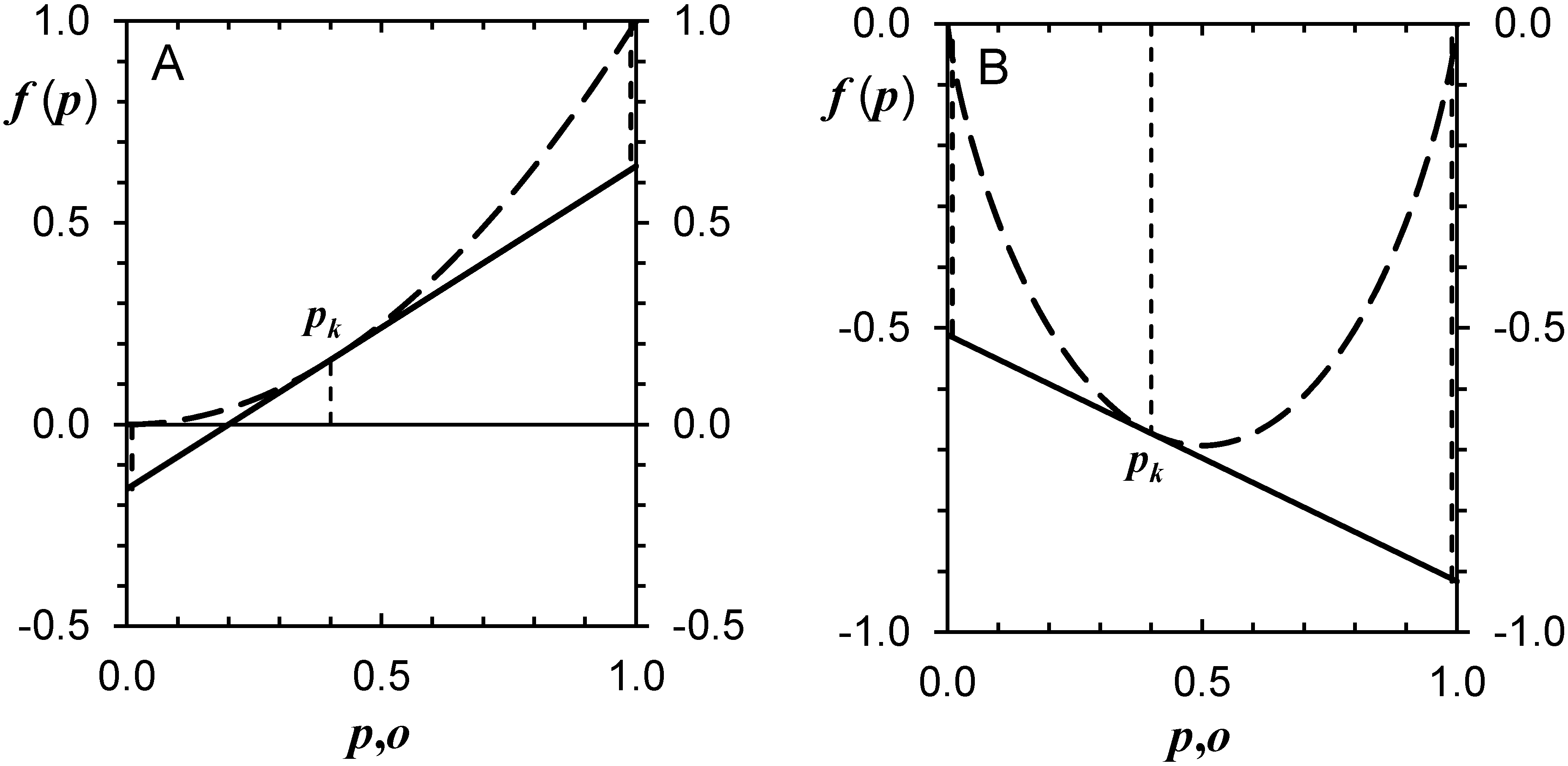
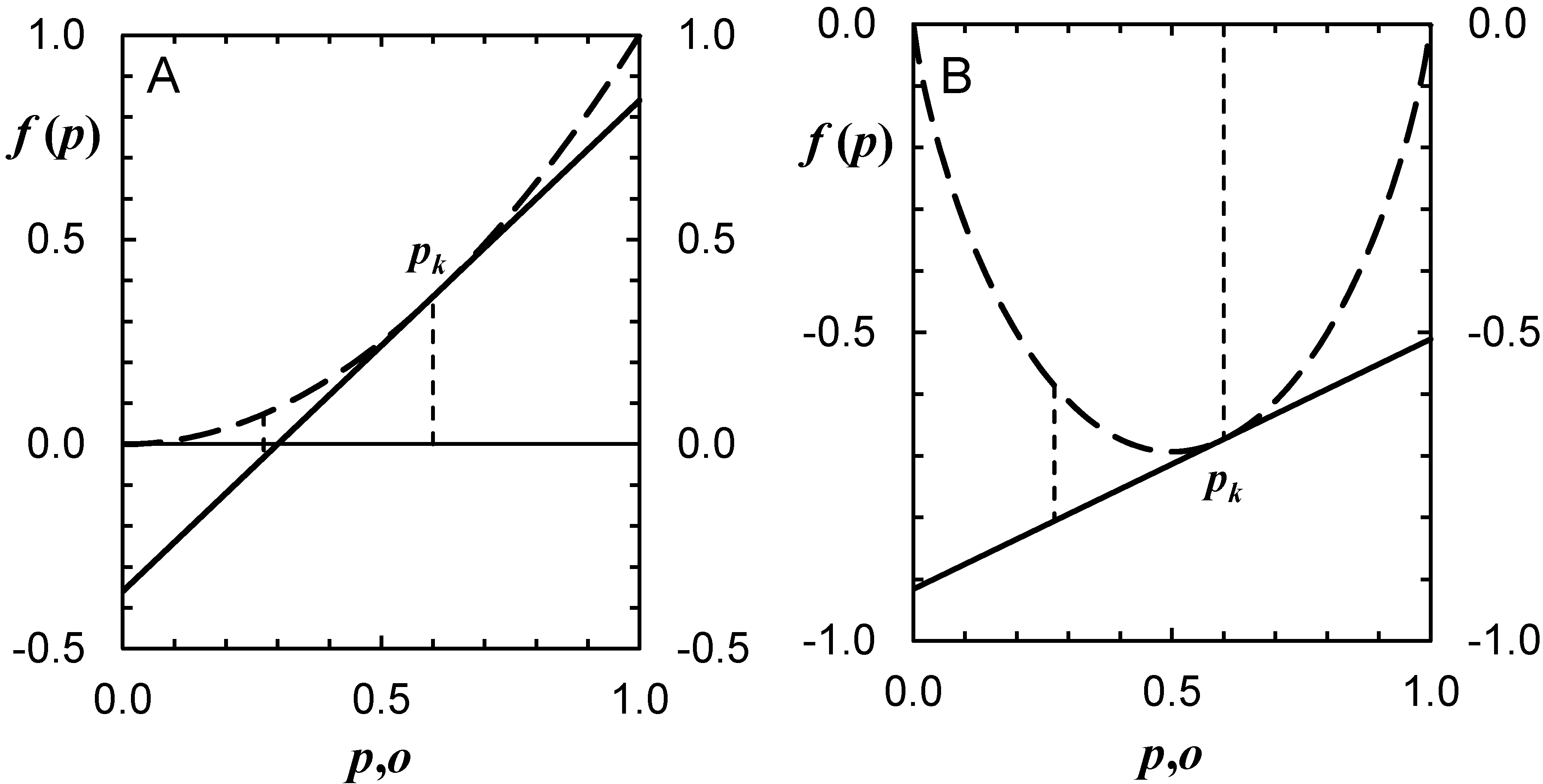
3.1.1. Brier Score and Divergence Score Diagrams for Individual Forecast Categories
- for o = 0, = 0.5108;
- for o = 1, = 0.9163.
3.1.2. Overall Scores

3.2. Reliability
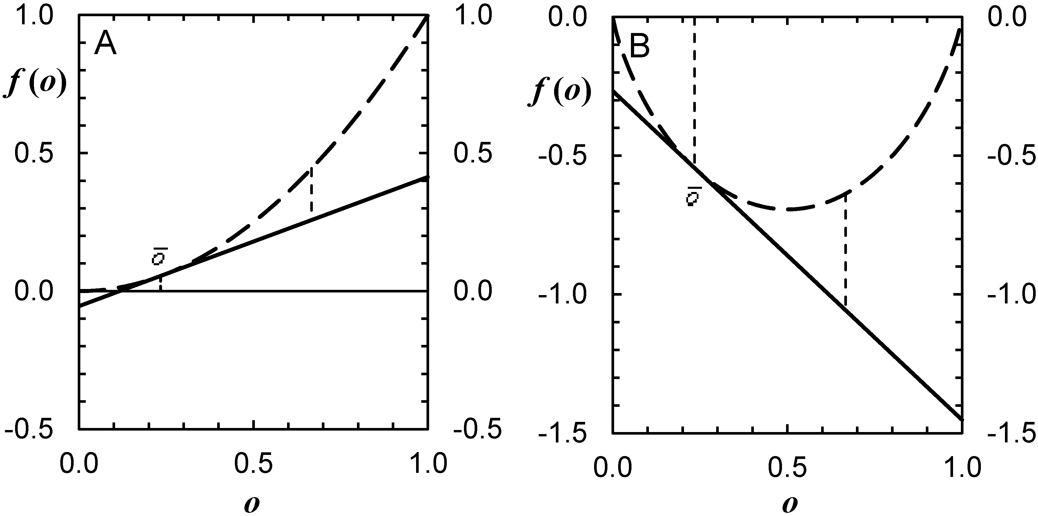
3.2.1. Reliability Diagrams for Individual Forecast Categories

3.2.2. Overall Reliability
3.2.3. Interpreting Reliability
3.3. Resolution
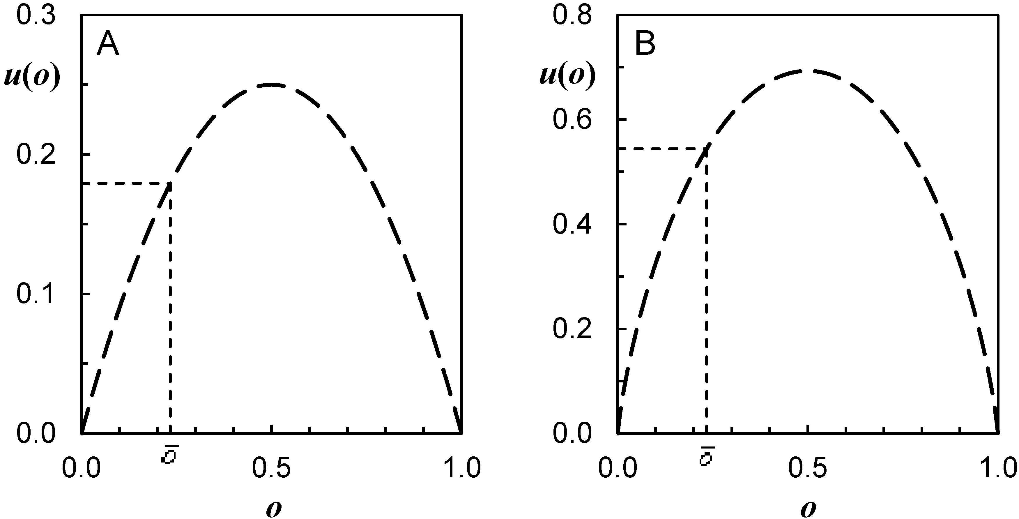
3.3.1. Resolution Diagrams for Individual Forecast Categories
3.3.2. Overall Resolution

3.3.3. Interpreting Resolution
3.4. Uncertainty

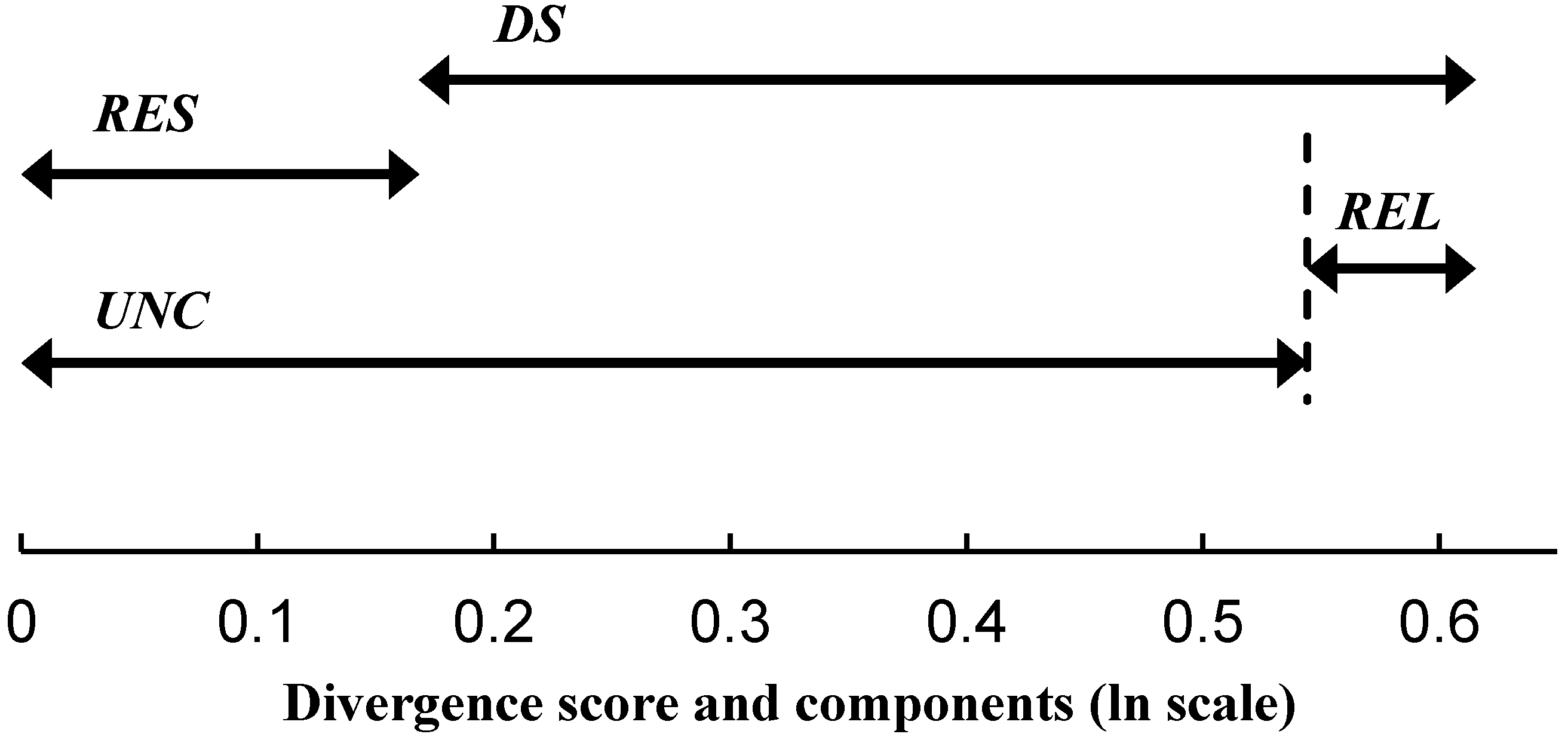
3.5. Overview
4. Discussion

Acknowledgments
Author Contributions
Conflicts of Interest
Appendix
| k | pk | nk | ok | nk/N | RELBS,k | RESBS,k | RELDS,k | RESDS,k | |
|---|---|---|---|---|---|---|---|---|---|
| 1 | 0.05 | 46 | 1 | 0.0217 | 0.1329 | 0.0367 | 2.0745 | 0.4862 | 8.6362 |
| 2 | 0.1 | 55 | 1 | 0.0182 | 0.1590 | 0.3682 | 2.5642 | 2.9939 | 10.8561 |
| 3 | 0.2 | 59 | 5 | 0.0847 | 0.1705 | 0.7837 | 1.3162 | 2.9746 | 4.5399 |
| 4 | 0.3 | 41 | 5 | 0.1220 | 0.1185 | 1.2998 | 0.5157 | 3.6576 | 1.6589 |
| 5 | 0.4 | 19 | 4 | 0.2105 | 0.0549 | 0.6821 | 0.0106 | 1.5491 | 0.0302 |
| 6 | 0.5 | 22 | 8 | 0.3636 | 0.0636 | 0.4091 | 0.3691 | 0.8286 | 0.9292 |
| 7 | 0.6 | 22 | 6 | 0.2727 | 0.0636 | 2.3564 | 0.0328 | 4.8346 | 0.0883 |
| 8 | 0.7 | 34 | 16 | 0.4706 | 0.0983 | 1.7894 | 1.9014 | 3.8702 | 4.5244 |
| 9 | 0.8 | 24 | 16 | 0.6667 | 0.0694 | 0.4267 | 4.4907 | 1.1695 | 10.0892 |
| 10 | 0.9 | 11 | 8 | 0.7273 | 0.0318 | 0.3282 | 2.6754 | 1.3052 | 5.9706 |
| 11 | 0.95 | 13 | 11 | 0.8462 | 0.0376 | 0.1402 | 4.8699 | 0.9745 | 10.9241 |
| Column sumsb | 346 | 81 | 1.0000 | 8.6204 | 20.8205 | 24.6439 | 58.2471 | ||
| k | pk | o | nk | f(o) | f(pk) | DB(0||pk) | ||
|---|---|---|---|---|---|---|---|---|
| 1 | 0.05 | 0 | 45 | 0.1 | 0 | 0.0025 | −0.0050 | 0.0025 |
| 2 | 0.1 | 0 | 54 | 0.2 | 0 | 0.0100 | −0.0200 | 0.0100 |
| 3 | 0.2 | 0 | 54 | 0.4 | 0 | 0.0400 | −0.0800 | 0.0400 |
| 4 | 0.3 | 0 | 36 | 0.6 | 0 | 0.0900 | −0.1800 | 0.0900 |
| 5b | 0.4 | 0 | 15 | 0.8 | 0 | 0.1600 | −0.3200 | 0.1600 |
| 6 | 0.5 | 0 | 14 | 1.0 | 0 | 0.2500 | −0.5000 | 0.2500 |
| 7 | 0.6 | 0 | 16 | 1.2 | 0 | 0.3600 | −0.7200 | 0.3600 |
| 8 | 0.7 | 0 | 18 | 1.4 | 0 | 0.4900 | −0.9800 | 0.4900 |
| 9 | 0.8 | 0 | 8 | 1.6 | 0 | 0.6400 | −1.2800 | 0.6400 |
| 10 | 0.9 | 0 | 3 | 1.8 | 0 | 0.8100 | −1.6200 | 0.8100 |
| 11 | 0.95 | 0 | 2 | 1.9 | 0 | 0.9025 | −1.8050 | 0.9025 |
| k | pk | o | nk | f(o) | f(pk) | DB(1||pk) | ||
|---|---|---|---|---|---|---|---|---|
| 1 | 0.05 | 1 | 1 | 0.1 | 1 | 0.0025 | 0.0950 | 0.9025 |
| 2 | 0.1 | 1 | 1 | 0.2 | 1 | 0.0100 | 0.1800 | 0.8100 |
| 3 | 0.2 | 1 | 5 | 0.4 | 1 | 0.0400 | 0.3200 | 0.4400 |
| 4 | 0.3 | 1 | 5 | 0.6 | 1 | 0.0900 | 0.4200 | 0.4900 |
| 5b | 0.4 | 1 | 4 | 0.8 | 1 | 0.1600 | 0.4800 | 0.3600 |
| 6 | 0.5 | 1 | 8 | 1.0 | 1 | 0.2500 | 0.5000 | 0.2500 |
| 7 | 0.6 | 1 | 6 | 1.2 | 1 | 0.3600 | 0.4800 | 0.1600 |
| 8 | 0.7 | 1 | 16 | 1.4 | 1 | 0.4900 | 0.4200 | 0.0900 |
| 9 | 0.8 | 1 | 16 | 1.6 | 1 | 0.6400 | 0.3200 | 0.0400 |
| 10 | 0.9 | 1 | 8 | 1.8 | 1 | 0.8100 | 0.1800 | 0.0100 |
| 11 | 0.95 | 1 | 11 | 1.9 | 1 | 0.9025 | 0.0950 | 0.0025 |
| k | pk | o | nk | f(o) | f(pk) | DB(0||pk) | ||
|---|---|---|---|---|---|---|---|---|
| 1 | 0.05 | 0 | 45 | −2.9444 | 0 | −0.1985 | 0.1472 | 0.0513 |
| 2 | 0.1 | 0 | 54 | −2.1972 | 0 | −0.3251 | 0.2197 | 0.1054 |
| 3 | 0.2 | 0 | 54 | −1.3863 | 0 | −0.5004 | 0.2773 | 0.2231 |
| 4 | 0.3 | 0 | 36 | −0.8473 | 0 | −0.6109 | 0.2542 | 0.3567 |
| 5b | 0.4 | 0 | 15 | −0.4055 | 0 | −0.6730 | 0.1622 | 0.5108 |
| 6 | 0.5 | 0 | 14 | 0.0000 | 0 | −0.6931 | 0.0000 | 0.6931 |
| 7 | 0.6 | 0 | 16 | 0.4055 | 0 | −0.6730 | −0.2433 | 0.9163 |
| 8 | 0.7 | 0 | 18 | 0.8473 | 0 | −0.6109 | −0.5931 | 1.2040 |
| 9 | 0.8 | 0 | 8 | 1.3863 | 0 | −0.5004 | −1.1090 | 1.6094 |
| 10 | 0.9 | 0 | 3 | 2.1972 | 0 | −0.3251 | −1.9775 | 2.3026 |
| 11 | 0.95 | 0 | 2 | 2.9444 | 0 | −0.1985 | −2.7972 | 2.9957 |
| k | pk | o | nk | f(o) | f(pk) | DB(1||pk) | ||
|---|---|---|---|---|---|---|---|---|
| 1 | 0.05 | 1 | 1 | −2.9444 | 0 | −0.1985 | −2.7972 | 2.9957 |
| 2 | 0.1 | 1 | 1 | −2.1972 | 0 | −0.3251 | −1.9775 | 2.3026 |
| 3 | 0.2 | 1 | 5 | −1.3863 | 0 | −0.5004 | −1.1090 | 1.6094 |
| 4 | 0.3 | 1 | 5 | −0.8473 | 0 | −0.6109 | −0.5931 | 1.2040 |
| 5b | 0.4 | 1 | 4 | −0.4055 | 0 | −0.6730 | −0.2433 | 0.9163 |
| 6 | 0.5 | 1 | 8 | 0.0000 | 0 | −0.6931 | 0.0000 | 0.6931 |
| 7 | 0.6 | 1 | 6 | 0.4055 | 0 | −0.6730 | 0.1622 | 0.5108 |
| 8 | 0.7 | 1 | 16 | 0.8473 | 0 | −0.6109 | 0.2542 | 0.3567 |
| 9 | 0.8 | 1 | 16 | 1.3863 | 0 | −0.5004 | 0.2773 | 0.2231 |
| 10 | 0.9 | 1 | 8 | 2.1972 | 0 | −0.3251 | 0.2197 | 0.1054 |
| 11 | 0.95 | 1 | 11 | 2.9444 | 0 | −0.1985 | 0.1472 | 0.0513 |
| k | pk | nk | f(pk) | |||||
|---|---|---|---|---|---|---|---|---|
| 1 | 0.05 | 0.0217 | 46 | 0.1 | 0.0005 | 0.0025 | −0.0028 | 0.0008 |
| 2 | 0.1 | 0.0182 | 55 | 0.2 | 0.0003 | 0.0100 | −0.0164 | 0.0067 |
| 3 | 0.2 | 0.0847 | 59 | 0.4 | 0.0072 | 0.0400 | −0.0461 | 0.0133 |
| 4 | 0.3 | 0.1220 | 41 | 0.6 | 0.0149 | 0.0900 | −0.1068 | 0.0317 |
| 5 | 0.4 | 0.2105 | 19 | 0.8 | 0.0443 | 0.1600 | −0.1516 | 0.0359 |
| 6 | 0.5 | 0.3636 | 22 | 1.0 | 0.1322 | 0.2500 | −0.1364 | 0.0186 |
| 7b | 0.6 | 0.2727 | 22 | 1.2 | 0.0744 | 0.3600 | −0.3927 | 0.1071 |
| 8 | 0.7 | 0.4706 | 34 | 1.4 | 0.2215 | 0.4900 | −0.3212 | 0.0526 |
| 9 | 0.8 | 0.6667 | 24 | 1.6 | 0.4444 | 0.6400 | −0.2133 | 0.0178 |
| 10 | 0.9 | 0.7273 | 11 | 1.8 | 0.5289 | 0.8100 | −0.3109 | 0.0298 |
| 11 | 0.95 | 0.8462 | 13 | 1.9 | 0.7160 | 0.9025 | −0.1973 | 0.0108 |
| k | pk | nk | f(pk) | |||||
|---|---|---|---|---|---|---|---|---|
| 1 | 0.05 | 0.0217 | 46 | −2.9444 | −0.1047 | −0.1985 | 0.0832 | 0.0106 |
| 2 | 0.1 | 0.0182 | 55 | −2.1972 | −0.0909 | −0.3251 | 0.1798 | 0.0544 |
| 3 | 0.2 | 0.0847 | 59 | −1.3863 | −0.2902 | −0.5004 | 0.1598 | 0.0504 |
| 4 | 0.3 | 0.1220 | 41 | −0.8473 | −0.3708 | −0.6109 | 0.1509 | 0.0892 |
| 5 | 0.4 | 0.2105 | 19 | −0.4055 | −0.5147 | −0.6730 | 0.0768 | 0.0815 |
| 6 | 0.5 | 0.3636 | 22 | 0.0000 | −0.6555 | −0.6931 | 0.0000 | 0.0377 |
| 7b | 0.6 | 0.2727 | 22 | 0.4055 | −0.5860 | −0.6730 | −0.1327 | 0.2198 |
| 8 | 0.7 | 0.4706 | 34 | 0.8473 | −0.6914 | −0.6109 | −0.1944 | 0.1138 |
| 9 | 0.8 | 0.6667 | 24 | 1.3863 | −0.6365 | −0.5004 | −0.1848 | 0.0487 |
| 10 | 0.9 | 0.7273 | 11 | 2.1972 | −0.5860 | −0.3251 | −0.3795 | 0.1187 |
| 11 | 0.95 | 0.8462 | 13 | 2.9444 | −0.4293 | −0.1985 | −0.3058 | 0.0750 |
| k | nk | |||||||
|---|---|---|---|---|---|---|---|---|
| 1 | 0.2341 | 0.0217 | 46 | 0.4682 | 0.0005 | 0.0548 | −0.0994 | 0.0451 |
| 2 | 0.2341 | 0.0182 | 55 | 0.4682 | 0.0003 | 0.0548 | −0.1011 | 0.0466 |
| 3 | 0.2341 | 0.0847 | 59 | 0.4682 | 0.0072 | 0.0548 | −0.0699 | 0.0223 |
| 4 | 0.2341 | 0.1220 | 41 | 0.4682 | 0.0149 | 0.0548 | −0.0525 | 0.0126 |
| 5 | 0.2341 | 0.2105 | 19 | 0.4682 | 0.0443 | 0.0548 | −0.0110 | 0.0006 |
| 6 | 0.2341 | 0.3636 | 22 | 0.4682 | 0.1322 | 0.0548 | 0.0606 | 0.0168 |
| 7 | 0.2341 | 0.2727 | 22 | 0.4682 | 0.0744 | 0.0548 | 0.0181 | 0.0015 |
| 8 | 0.2341 | 0.4706 | 34 | 0.4682 | 0.2215 | 0.0548 | 0.1107 | 0.0559 |
| 9b | 0.2341 | 0.6667 | 24 | 0.4682 | 0.4444 | 0.0548 | 0.2025 | 0.1871 |
| 10 | 0.2341 | 0.7273 | 11 | 0.4682 | 0.5289 | 0.0548 | 0.2309 | 0.2432 |
| 11 | 0.2341 | 0.8462 | 13 | 0.4682 | 0.7160 | 0.0548 | 0.2866 | 0.3746 |
| k | nk | |||||||
|---|---|---|---|---|---|---|---|---|
| 1 | 0.2341 | 0.0217 | 46 | −1.1853 | −0.1047 | −0.5442 | 0.2517 | 0.1877 |
| 2 | 0.2341 | 0.0182 | 55 | −1.1853 | −0.0909 | −0.5442 | 0.2559 | 0.1974 |
| 3 | 0.2341 | 0.0847 | 59 | −1.1853 | −0.2902 | −0.5442 | 0.1770 | 0.0769 |
| 4 | 0.2341 | 0.1220 | 41 | −1.1853 | −0.3708 | −0.5442 | 0.1329 | 0.0405 |
| 5 | 0.2341 | 0.2105 | 19 | −1.1853 | −0.5147 | −0.5442 | 0.0279 | 0.0016 |
| 6 | 0.2341 | 0.3636 | 22 | −1.1853 | −0.6555 | −0.5442 | −0.1535 | 0.0422 |
| 7 | 0.2341 | 0.2727 | 22 | −1.1853 | −0.5860 | −0.5442 | −0.0458 | 0.0040 |
| 8 | 0.2341 | 0.4706 | 34 | −1.1853 | −0.6914 | −0.5442 | −0.2803 | 0.1331 |
| 9b | 0.2341 | 0.6667 | 24 | −1.1853 | −0.6365 | −0.5442 | −0.5127 | 0.4204 |
| 10 | 0.2341 | 0.7273 | 11 | −1.1853 | −0.5860 | −0.5442 | −0.5845 | 0.5428 |
| 11 | 0.2341 | 0.8462 | 13 | −1.1853 | −0.4293 | −0.5442 | −0.7255 | 0.8403 |
References
- Lindley, D.V. Making Decisions, 2nd ed.; Wiley: Chichester, UK, 1985. [Google Scholar]
- Jolliffe, I.T.; Stephenson, D.B. (Eds.) Forecast Verification: A Practitioner’s Guide in Atmospheric Science, 2nd ed.; Wiley: Chichester, UK, 2012.
- Broecker, J. Probability forecasts. In Forecast Verification: A Practitioner’s Guide in Atmospheric Science, 2nd ed.; Jolliffe, I.T., Stephenson, D.B., Eds.; Wiley: Chichester, UK, 2012; pp. 119–139. [Google Scholar]
- Brier, G.W. Verification of forecasts expressed in terms of probability. Mon. Weather Rev. 1950, 78, 1–3. [Google Scholar] [CrossRef]
- Good, I.J. Rational decisions. J. Roy. Stat. Soc. B 1952, 14, 107–114. [Google Scholar]
- DeGroot, M.W.; Fienberg, S.E. The comparison and evaluation of forecasters. The Statistician 1983, 32, 12–22. [Google Scholar] [CrossRef]
- Bröcker, J.; Smith, L.A. Scoring probabilistic forecasts: the importance of being proper. Weather Forecast. 2007, 22, 382–388. [Google Scholar] [CrossRef]
- Bröcker, J. Reliability, sufficiency, and the decomposition of proper scores. Q. J. R. Meteorol. Soc. 2009, 135, 1512–1519. [Google Scholar] [CrossRef]
- Murphy, A.H. A new vector partition of the probability score. J. Appl. Meteorol. 1973, 12, 595–600. [Google Scholar] [CrossRef]
- Wilks, D.S. Statistical Methods in the Atmospheric Sciences, 3rd ed.; Academic Press: Oxford, UK, 2011. [Google Scholar]
- Weijs, S.V.; Schoups, G.; van de Giesen, N. Why hydrological predictions should be evaluated using information theory. Hydrol. Earth Syst. Sci. 2010, 14, 2545–2558. [Google Scholar] [CrossRef]
- Weijs, S.V.; van Nooijen, R.; van de Giesen, N. Kullback-Leibler divergence as a forecast skill score with classic reliability-resolution-uncertainty decomposition. Mon. Weather Rev. 2010, 138, 3387–3399. [Google Scholar] [CrossRef]
- Gneiting, T.; Katzfuss, M. Probabilistic forecasting. Annu. Rev. Stat. Appl. 2014, 1, 125–151. [Google Scholar] [CrossRef]
- Verifying probability of precipitation—an example from Finland. http://www.cawcr.gov.au/projects/verification/POP3/POP3.html (accessed on 18 June 2015).
- Kullback, S. Information Theory and Statistics, 2nd ed.; Dover: New York, NY, USA, 1968. [Google Scholar]
- Cover, T.M.; Thomas, J.A. Elements of Information Theory, 2nd ed.; Wiley: Hoboken, NJ, USA, 2006. [Google Scholar]
- Shannon, C.E.; Weaver, W. The Mathematical Theory of Communication; University of Illinois Press: Urbana, IL, USA, 1949. [Google Scholar]
- Bregman, L.M. The relaxation method of finding the common points of convex sets and its application to the solution of problems in convex programming. USSR Comput. Math. Math. Phys. 1967, 7, 200–217. [Google Scholar] [CrossRef]
- Gneiting, T.; Raftery, A.E. Strictly proper scoring rules, prediction, and estimation. J. Am. Stat. Assoc. 2007, 102, 359–378. [Google Scholar] [CrossRef]
- Adamčik, M. The information geometry of Bregman divergences and some applications in multi-expert reasoning. Entropy 2014, 16, 6338–6381. [Google Scholar] [CrossRef]
- Reid, M.D.; Williamson, R.C. Information, divergence and risk for binary experiments. J. Mach. Learn. Res. 2011, 12, 731–817. [Google Scholar]
- Banerjee, A.; Merugu, S.; Dhillon, I.S.; Ghosh, J. Clustering with Bregman divergences. J. Mach. Learn. Res. 2005, 6, 1705–1749. [Google Scholar]
- Theil, H. Statistical Decomposition Analysis; North-Holland Publishing Company: Amsterdam, The Netherlands, 1972. [Google Scholar]
- Benedetti, R. Scoring rules for forecast verification. Mon. Weather Rev. 2010, 138, 203–211. [Google Scholar] [CrossRef]
- Tödter, J.; Ahrens, B. Generalization of the ignorance score: continuous ranked version and its decomposition. Mon. Weather Rev. 2012, 140, 2005–2017. [Google Scholar] [CrossRef]
- Topp, C.F.E.; Wang, W.; Cloy, J.M.; Rees, R.M.; Hughes, G. Information properties of boundary line models for N2O emissions from agricultural soils. Entropy 2013, 15, 972–987. [Google Scholar] [CrossRef]
- Cardenas, L.M.; Gooday, R.; Brown, L.; Scholefield, D.; Cuttle, S.; Gilhespy, S.; Matthews, R.; Misselbrook, T.; Wang, J.; Li, C.; Hughes, G.; Lord, E. Towards an improved inventory of N2O from agriculture: model evaluation of N2O emission factors and N fraction leached from different sources in UK agriculture. Atmos. Environ. 2013, 79, 340–348. [Google Scholar] [CrossRef]
- Rees, R.M.; Augustin, J.; Alberti, G.; Ball, B.C.; Boeckx, P.; Cantarel, A.; Castaldi, S.; Chirinda, N.; Chojnicki, B.; Giebels, M.; Gordon, H.; Grosz, B.; Horvath, L.; Juszczak, R.; Klemedtsson, Å.K.; Klemedtsson, L.; Medinets, S.; Machon, A.; Mapanda, F.; Nyamangara, J.; Olesen, J.E.; Reay, D.S.; Sanchez, L.; Sanz Cobena, A.; Smith, K.A.; Sowerby, A.; Sommer, J.M.; Soussana, J.F.; Stenberg, M.; Topp, C.F.E.; van Cleemput, O.; Vallejo, A.; Watson, C.A.; Wuta, M. Nitrous oxide emissions from European agriculture—an analysis of variability and drivers of emissions from field experiments. Biogeosciences 2013, 10, 2671–2682. [Google Scholar]
- Hawkins, M.J.; Hyde, B.P.; Ryan, M.; Schulte, R.P.O.; Connolly, J. An empirical model and scenario analysis of nitrous oxide emissions from a fertilised and grazed grassland site in Ireland. Nutr. Cycl. Agroecosyst. 2007, 79, 93–101. [Google Scholar] [CrossRef]
- Moran, D.; Lucas, A.; Barnes, A. Mitigation win-win. Nat. Clim. Change 2013, 3, 611–613. [Google Scholar] [CrossRef]
© 2015 by the authors; licensee MDPI, Basel, Switzerland. This article is an open access article distributed under the terms and conditions of the Creative Commons Attribution license (http://creativecommons.org/licenses/by/4.0/).
Share and Cite
Hughes, G.; Topp, C.F.E. Probabilistic Forecasts: Scoring Rules and Their Decomposition and Diagrammatic Representation via Bregman Divergences. Entropy 2015, 17, 5450-5471. https://doi.org/10.3390/e17085450
Hughes G, Topp CFE. Probabilistic Forecasts: Scoring Rules and Their Decomposition and Diagrammatic Representation via Bregman Divergences. Entropy. 2015; 17(8):5450-5471. https://doi.org/10.3390/e17085450
Chicago/Turabian StyleHughes, Gareth, and Cairistiona F.E. Topp. 2015. "Probabilistic Forecasts: Scoring Rules and Their Decomposition and Diagrammatic Representation via Bregman Divergences" Entropy 17, no. 8: 5450-5471. https://doi.org/10.3390/e17085450