
A Five Species Cyclically Dominant Evolutionary Game with Fixed Direction: A New Way to Produce Self-Organized Spatial Patterns

Abstract
:
1. Introduction
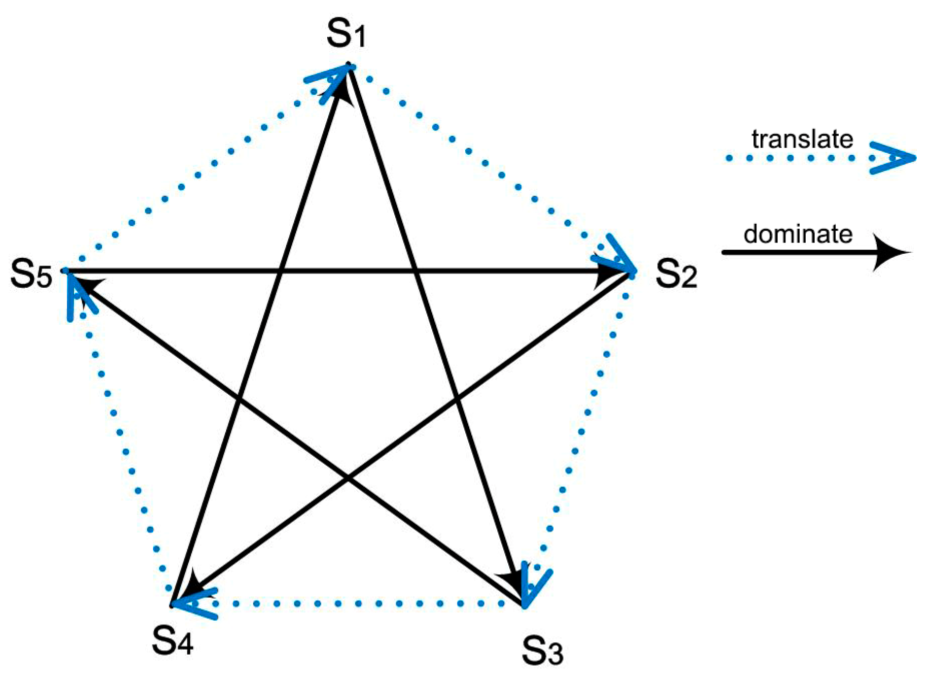
2. Model
- Place individuals using different strategies randomly on the lattice;
- For each individual using the strategy Si in the system, count the numbers of Si-1 and Si-2 respectively in its neighbors. If the number of Si-2 in its neighbors is more than Si-1, we label the individual Si as “alterable”.
- Changing the labeled “alterable” individuals’ strategies from Si to Si+1.
- Repeat step 2.
3. Mean Field Theory
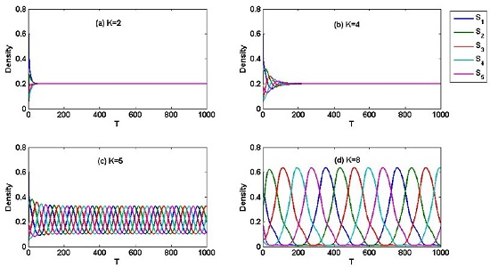
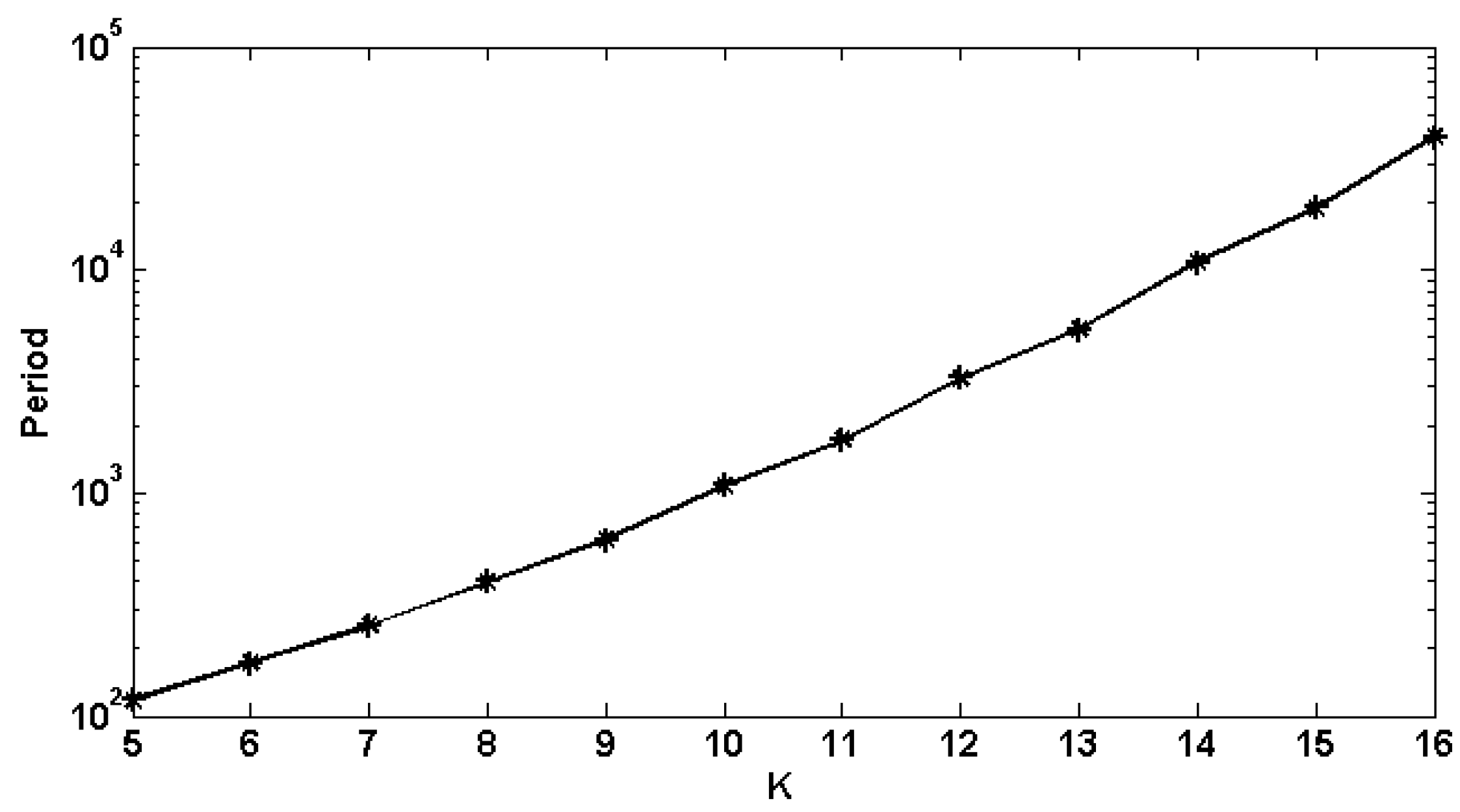
4. Numerical Result
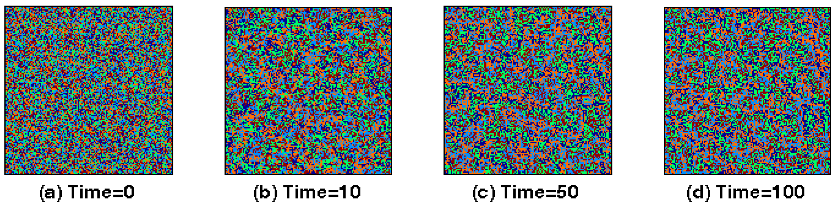
5. Simulation
6. Conclusions
Acknowledgments
Author Contributions
Conflicts of Interest
References
- Czaran, T.L.; Hoekstra, R.F.; Pagie, L. Chemical warfare between microbes promotes biodiversity. Proc. Natl. Acad. Sci. USA 2002, 99, 786–790. [Google Scholar] [CrossRef] [PubMed]
- Kerr, B.; Riley, M.A.; Feldman, M.W.; Bohannan, B.J.M. Local dispersal promotes biodiversity in a real-life game of rock–paper–scissors. Nature 2002, 418, 171–174. [Google Scholar] [CrossRef] [PubMed]
- Reichenbach, T.; Mobilia, M.; Frey, E. Mobility promotes and jeopardizes biodiversity in rock–paper–scissors games. Nature 2007, 448, 1046–1049. [Google Scholar] [CrossRef] [PubMed]
- Reichenbach, T.; Mobilia, M.; Frey, E. Coexistence versus extinction in the stochastic cyclic Lotka–Volterra model. Phys. Rev. E 2006, 74, 051907. [Google Scholar] [CrossRef] [PubMed]
- Claussen, J.C.; Traulsen, A. Cyclic dominance and biodiversity in well-mixed populations. Phys. Rev. Lett. 2008, 100, 058104. [Google Scholar] [CrossRef] [PubMed]
- Weber, M.F.; Poxleitner, G.; Hebisch, E.; Frey, E.; Opitz, M. Chemical warfare and survival strategies in bacterial range expansions. J. R. Soc. Interface 2014, 11, 20140172. [Google Scholar] [CrossRef] [PubMed]
- Jackson, J.B.C.; Buss, L. Alleopathy and spatial competition among coral reef invertebrates. Proc. Natl. Acad. Sci. USA 1975, 72, 5160–5163. [Google Scholar] [CrossRef] [PubMed]
- Taylor, D.R.; Aarssen, L.W. Complex competitive relationships among genotypes of three perennial grasses: Implications for species coexistence. Am. Nat. 1990, 136, 305–327. [Google Scholar] [CrossRef]
- Silvertown, J.; Holtier, S.; Johnson, J.; Dale, P. Cellular automaton models of interspecific competition for space—The effect of pattern on process. J. Ecol. 1992, 80, 527–534. [Google Scholar] [CrossRef]
- Durrett, R.; Levin, S. Spatial aspects of interspecific competition. Theor. Popul. Biol. 1998, 53, 30–43. [Google Scholar] [CrossRef] [PubMed]
- Lankau, R.A.; Strauss, S.Y. Mutual feedbacks maintain both genetic and species diversity in a plant community. Science 2007, 317, 1561–1563. [Google Scholar] [CrossRef] [PubMed]
- Cameron, D.D.; White, A.; Antonovics, J. Parasite–grass–forb interactions and rock–paper–scissor dynamics: Predicting the effects of the parasitic plant Rhinanthus minor on host plant communities. J. Ecol. 2009, 97, 1311–1319. [Google Scholar] [CrossRef]
- Durrett, R.; Levin, S. Allelopathy in spatially distributed populations. J. Theor. Biol. 1997, 185, 165–171. [Google Scholar] [CrossRef] [PubMed]
- Kirkup, B.C.; Riley, M.A. Antibiotic-mediated antagonism leads to a bacterial game of rock–paper–scissors in vivo. Nature 2004, 428, 412–414. [Google Scholar] [CrossRef] [PubMed]
- Neumann, G.F.; Jetschke, G. Evolutionary classification of toxin mediated interactions in microorganisms. Biosystems 2010, 99, 155–166. [Google Scholar] [CrossRef] [PubMed]
- Nahum, J.R.; Harding, B.N.; Kerr, B. Evolution of restraint in a structured rock–paper–scissors community. Proc. Natl. Acad. Sci. USA 2011, 108, 10831–10838. [Google Scholar] [CrossRef] [PubMed]
- Knebel, J.; Weber, M.F.; Krüger, T.; Frey, E. Evolutionary games of condensates in coupled birth-death processes. Nat. Commun. 2015, 6, 6977. [Google Scholar] [CrossRef] [PubMed]
- Sinervo, B.; Lively, C.M. The rock-paper-scissors game and the evolution of alternative male strategies. Nature 1996, 380, 240–243. [Google Scholar] [CrossRef]
- Gilg, O.; Hanski, I.; Sittler, B. Cyclic dynamics in a simple vertebrate predator-prey community. Science 2003, 302, 866–868. [Google Scholar] [CrossRef] [PubMed]
- Guill, C.; Drossel, B.; Just, W.; Carmack, E. A three-species model explaining cyclic dominance of Pacific salmon. J. Theor. Biol. 2011, 276, 16–21. [Google Scholar] [CrossRef] [PubMed]
- Berlow, E.L.; Neutel, A.M.; Cohen, J.E.; de Ruiter, P.C.; Ebenman, B.; Emmerson, M.; Fox, J.W.; Jansen, V.A.A.; Jones, J.I.; Kokkoris, G.D.; et al. Interaction strengths in food webs: Issues and opportunities. J. Anim. Ecol. 2004, 73, 585–598. [Google Scholar] [CrossRef]
- Stouffer, D.B.; Sales-Pardo, M.; Sirer, M.I.; Bascompte, J. Evolutionary Conservation of Species’ Roles in Food Webs. Science 2012, 335, 1489–1492. [Google Scholar] [CrossRef] [PubMed]
- Avelino, P.P.; Bazeia, D.; Menezes, J.; de Oliveira, B.F. String networks in ZN Lotka–Volterra competition models. Phys. Lett. A 2014, 378, 393–397. [Google Scholar] [CrossRef]
- Dobrinevski, A.; Alava, M.; Reichenbach, T.; Frey, E. Mobility-dependent selection of competing strategy associations. Phys. Rev. E 2014, 89, 012721. [Google Scholar] [CrossRef] [PubMed]
- Durney, C.H.; Case, S.O.; Pleimling, M.; Zia, R.K.P. Saddles, arrows, and spirals: Deterministic trajectories in cyclic competition of four species. Phys. Rev. E 2011, 83, 051108. [Google Scholar] [CrossRef] [PubMed]
- Feng, S.S.; Qiang, C.C. Self-organization of five species in a cyclic competition game. Physica A 2013, 392, 4675–4682. [Google Scholar] [CrossRef]
- Intoy, B.; Pleimling, M. Extinction in four species cyclic competition. J. Stat. Mech. Theory Exp. 2013, 16, P08011. [Google Scholar] [CrossRef]
- Kang, Y.B.; Pan, Q.H.; Wang, X.T.; He, M.F. A golden point rule in rock-paper-scissors-lizard-spock game. Physica A 2013, 392, 2652–2659. [Google Scholar] [CrossRef]
- Vukov, J.; Szolnoki, A.; Szabo, G. Diverging fluctuations in a spatial five-species cyclic dominance game. Phys. Rev. E 2013, 88, 022123. [Google Scholar] [CrossRef] [PubMed]
- Szolnoki, A.; Mobilia, M.; Jiang, L.L.; Szczesny, B.; Rucklidge, A.M.; Perc, M. Cyclic dominance in evolutionary games: A review. J. R. Soc. Interface 2014, 11, 20140735. [Google Scholar] [CrossRef] [PubMed]
- Cheng, H.Y.; Yao, N.; Huang, Z.G.; Park, J.; Do, Y.; Lai, Y.C. Mesoscopic Interactions and Species Coexistence in Evolutionary Game Dynamics of Cyclic Competitions. Sci. Rep. 2014, 4, 7486. [Google Scholar] [CrossRef] [PubMed]
- Knebel, J.; Kruger, T.; Weber, M.F.; Frey, E. Coexistence and Survival in Conservative Lotka–Volterra Networks. Phys. Rev. Lett. 2013, 110, 168106. [Google Scholar] [CrossRef] [PubMed]
- Laird, R.A.; Schamp, B.S. Species coexistence, intransitivity, and topological variation in competitive tournaments. J. Theor. Biol. 2009, 256, 90–95. [Google Scholar] [CrossRef] [PubMed]
- Li, Y.M.; Dong, L.R.; Yang, G.C. The elimination of hierarchy in a completely cyclic competition system. Physica A 2012, 391, 125–131. [Google Scholar] [CrossRef]
- Andrae, B.; Cremer, J.; Reichenbach, T.; Frey, E. Entropy production of cyclic population dynamics. Phys. Rev. Lett. 2010, 104, 218102. [Google Scholar] [CrossRef] [PubMed]
- Mobilia, M. Oscillatory dynamics in rock–paper–scissors games with mutations. J. Theor. Biol. 2010, 264, 1–10. [Google Scholar] [CrossRef] [PubMed]
- LiLing, J. Human Phenome Based on Traditional Chinese Medicine—A Solution to Congenital Syndromology. Am. J. Chin. Med. 2012, 31, 991–1000. [Google Scholar] [CrossRef] [PubMed]
- Wu Xing. Available online: https://en.wikipedia.org/wiki/Wu_Xing (accessed on 2 August 2016).
- Santos, F.P.; Encarnação, S.; Santos, F.C.; Portugali, J.; Pacheco, J.M. An Evolutionary Game Theoretic Approach to Multi-Sector Coordination and Self-Organization. Entropy 2016, 18, 152. [Google Scholar] [CrossRef]
- Boerlijst, M.; Hogeweg, P. Spiral wave structure in pre-biotic evolution: HyPercycles stable against parasites. Physica D 1991, 48, 17–28. [Google Scholar] [CrossRef]
- Boerlijst, M.C.; Lamers, M.; Hogeweg, P. Evolutionary consequences of spiral patterns in a host-parasitoid system. Proc. R. Soc. Lond. B 1993, 253, 15–18. [Google Scholar] [CrossRef]
- Roman, A.; Dasgupta, D.; Pleimling, M. A theoretical approach to understand spatial organization in complex ecologies. J. Theor. Biol. 2016, 403, 10–16. [Google Scholar] [CrossRef] [PubMed]
- Hofbauer, J.; Sigmund, K. Evolutionary Games and Population Dynamics; Cambridge University Press: Cambridge, UK, 1998. [Google Scholar]
- Szczesny, B. Coevolutionary Dynamics in Structured Populations of Three Species. Ph.D. Thesis, University of Leeds, Leeds, UK, 2014. [Google Scholar]


© 2016 by the authors; licensee MDPI, Basel, Switzerland. This article is an open access article distributed under the terms and conditions of the Creative Commons Attribution (CC-BY) license (http://creativecommons.org/licenses/by/4.0/).
Share and Cite
Kang, Y.; Pan, Q.; Wang, X.; He, M. A Five Species Cyclically Dominant Evolutionary Game with Fixed Direction: A New Way to Produce Self-Organized Spatial Patterns. Entropy 2016, 18, 284. https://doi.org/10.3390/e18080284
Kang Y, Pan Q, Wang X, He M. A Five Species Cyclically Dominant Evolutionary Game with Fixed Direction: A New Way to Produce Self-Organized Spatial Patterns. Entropy. 2016; 18(8):284. https://doi.org/10.3390/e18080284
Chicago/Turabian StyleKang, Yibin, Qiuhui Pan, Xueting Wang, and Mingfeng He. 2016. "A Five Species Cyclically Dominant Evolutionary Game with Fixed Direction: A New Way to Produce Self-Organized Spatial Patterns" Entropy 18, no. 8: 284. https://doi.org/10.3390/e18080284
APA StyleKang, Y., Pan, Q., Wang, X., & He, M. (2016). A Five Species Cyclically Dominant Evolutionary Game with Fixed Direction: A New Way to Produce Self-Organized Spatial Patterns. Entropy, 18(8), 284. https://doi.org/10.3390/e18080284