
Short Term Electrical Load Forecasting Using Mutual Information Based Feature Selection with Generalized Minimum-Redundancy and Maximum-Relevance Criteria

Abstract
:1. Introduction
2. Methodology
2.1. Mutual Information-Based Generalized Minimal-Redundancy and Maximal-Relevance
2.2. Random Forest
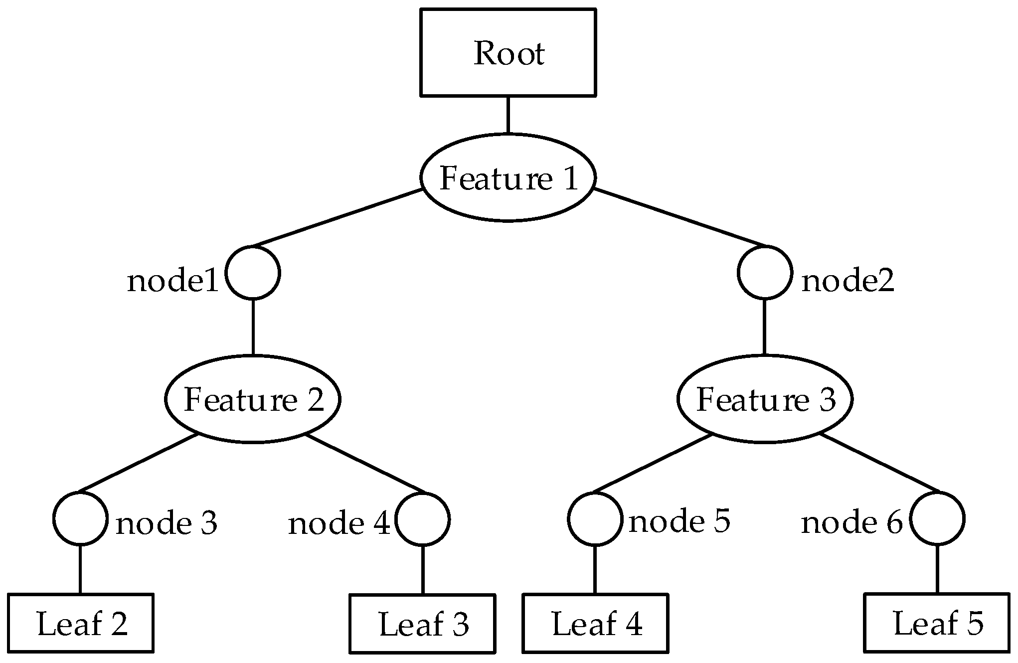
2.2.1. CART
2.2.2. Bagging
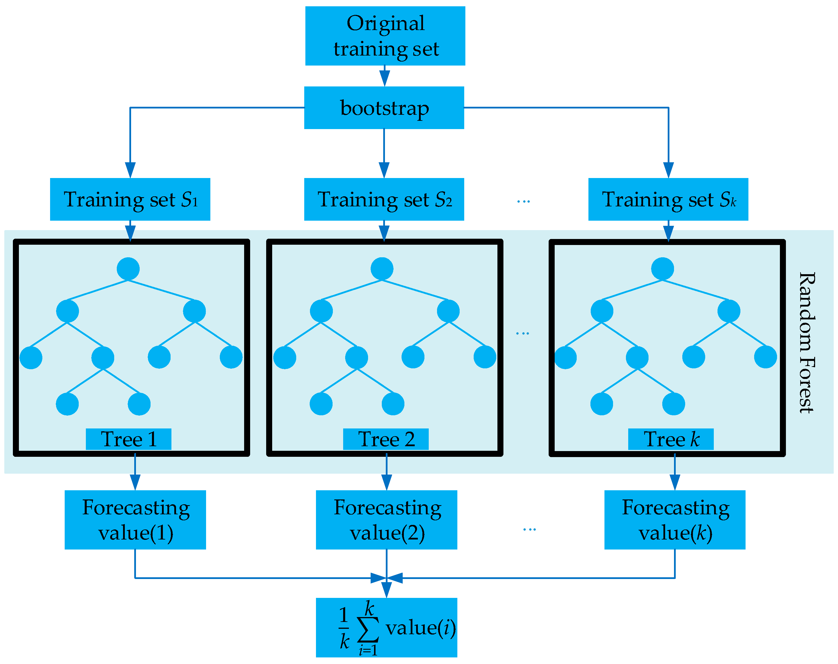
2.2.3. RF
- (1)
- k training sets are sampled with replacement from the dataset B by bootstrap.
- (2)
- Each training set grows up to a tree according to CART algorithm. Supposing dataset B has M features and mtry features are randomly selected from B for each non-leaf node. Afterward, the node is split by a feature selected from these mtry features.
- (3)
- Each tree grows completely without pruning.
- (4)
- The forecasting result is solved by calculating the mean value of the consequences of each tree predicted.
- (1)
- The same capacity of the training set sampled by bootstrap guarantees each sample in dataset B to be appraised equally. A situation that one sample may appear many times in the same training set and some may not causes low correlation among the trees.
- (2)
- The manner of selecting feature for node split applies randomness, and ensures the generalized performance of RF.
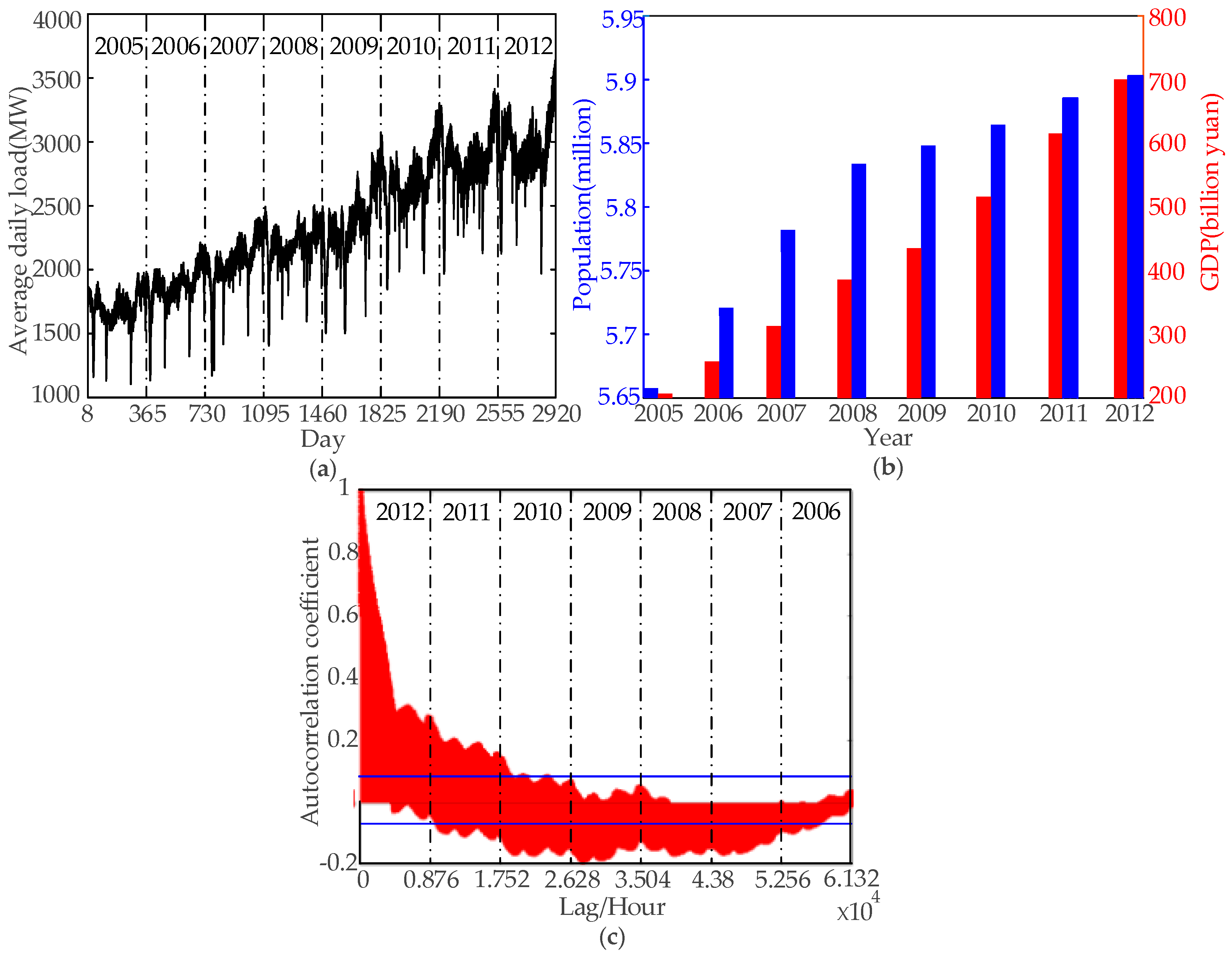
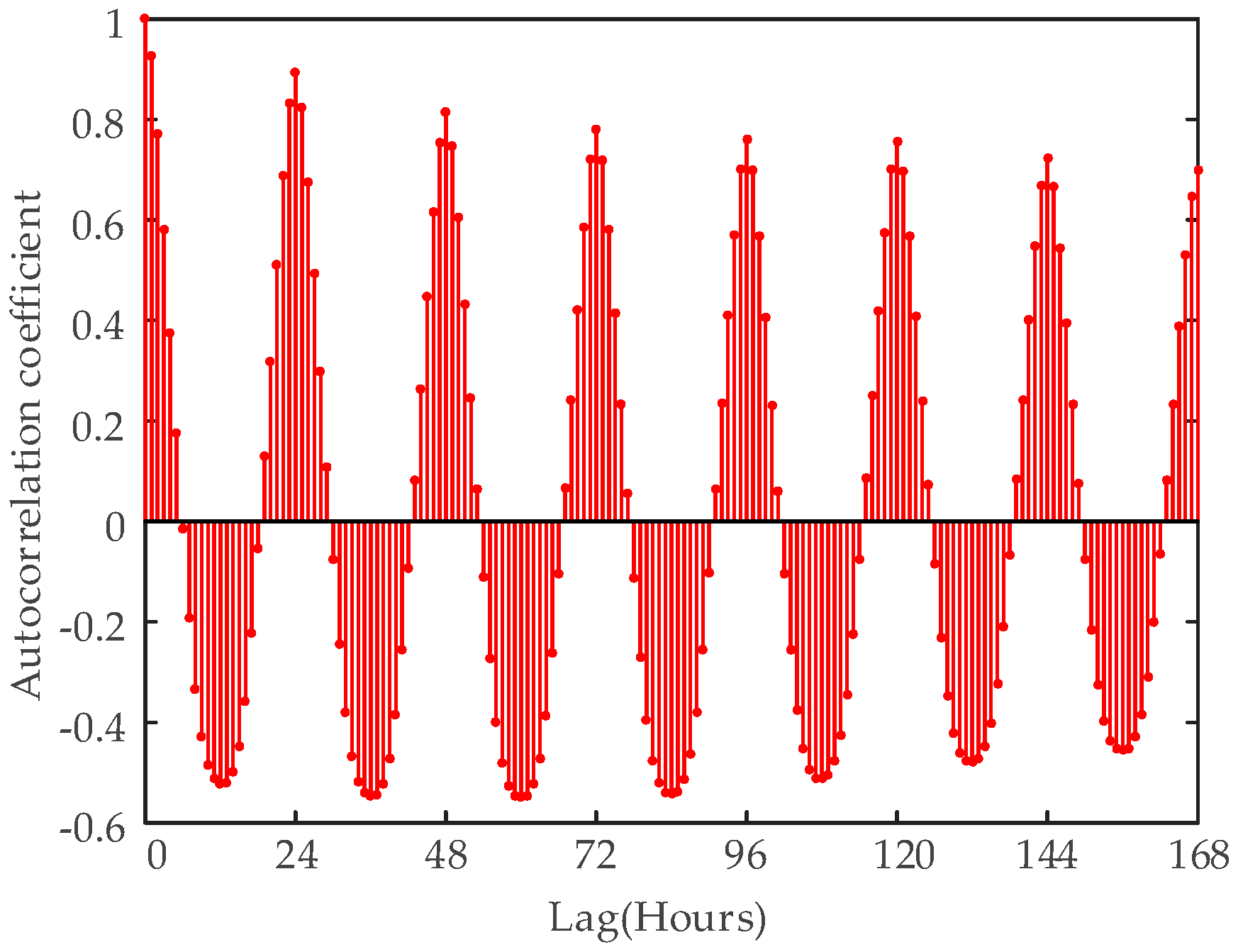
3. Data Analysis
- FHour means the moment of hour, which is tagged by the numbers from 1 to 24.
- FWW is either weekday or weekend marked by binary numbers, wherein 0 means weekend and 1 means weekday.
- FDW refers to the day of week, which is labeled by the numbers from 1 to 7.
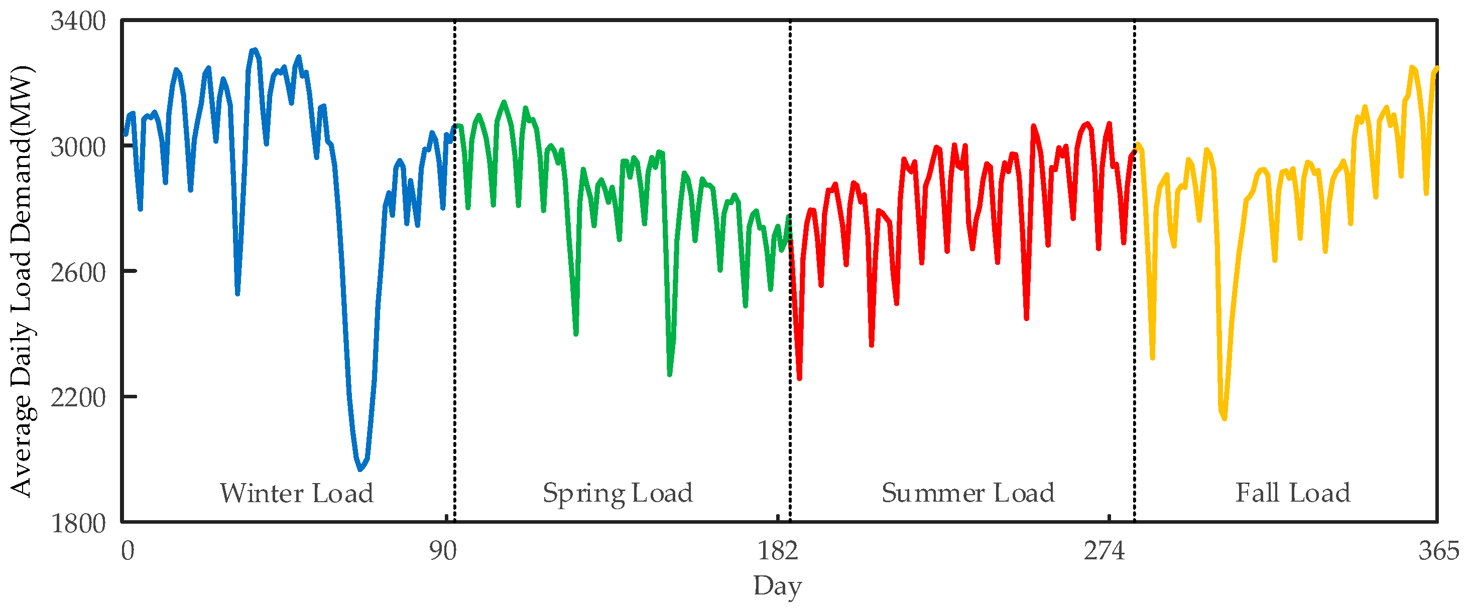
- FS uses the numbers from 1 to 4.
- FL(t-25) is the load 25 h before, FL(t-26) means the load 26 h before, and so on.
4. The Proposed Feature Selection Method and STLF Model
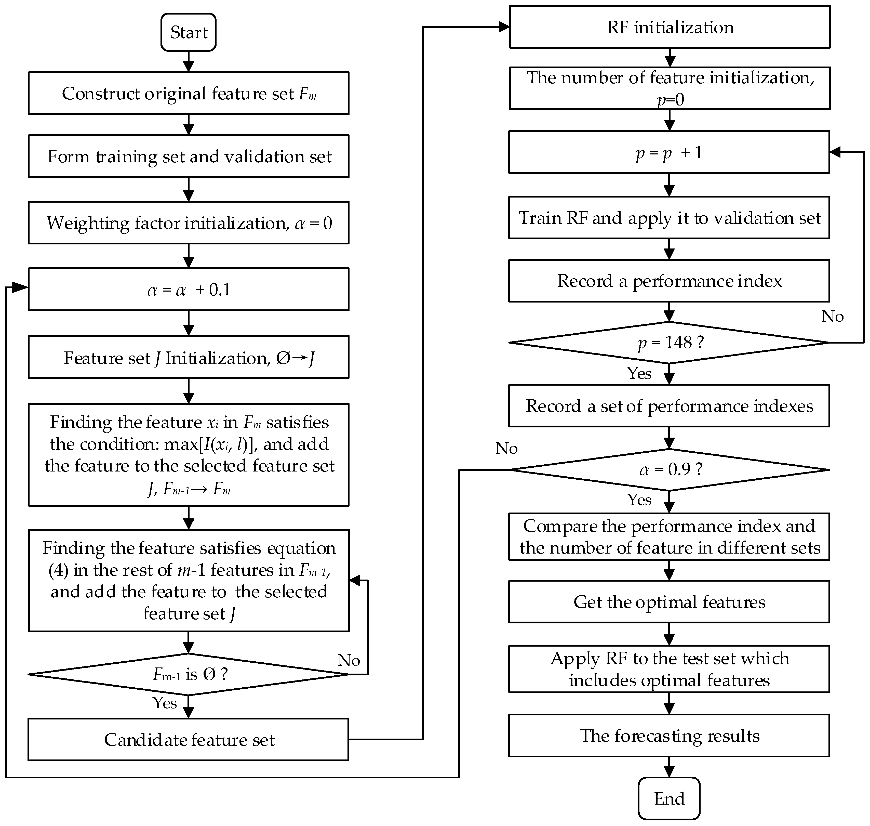
4.1. G-mRMR for Feature Selection
- (1)
- Initialization Ø→J.
- (2)
- Compute the relevance between each feature and target variable l. Pick out the feature from Fm which satisfies Equation (2) and add it into J.
- (3)
- Find the feature in the rest of m−1 features in Fm that satisfies Equation (4) and add it in to J.
- (4)
- Repeat step (3) until Fm becomes Ø.
- (5)
- Rank the features in feature set J in descending order in accordance with the measured mRMR value.
4.2. Wrapper for Feature Selection
4.3. The Proposed STLF Model
5. Case Study and Results Analysis
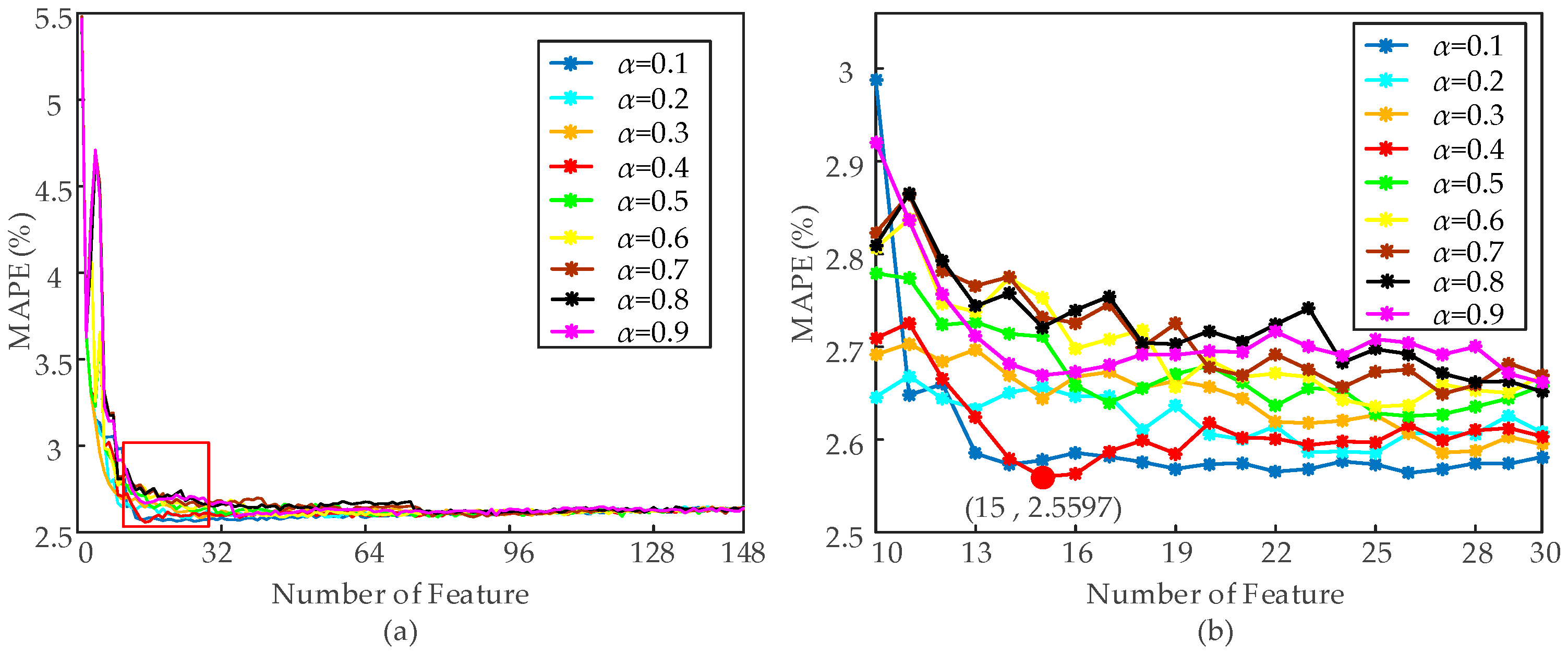
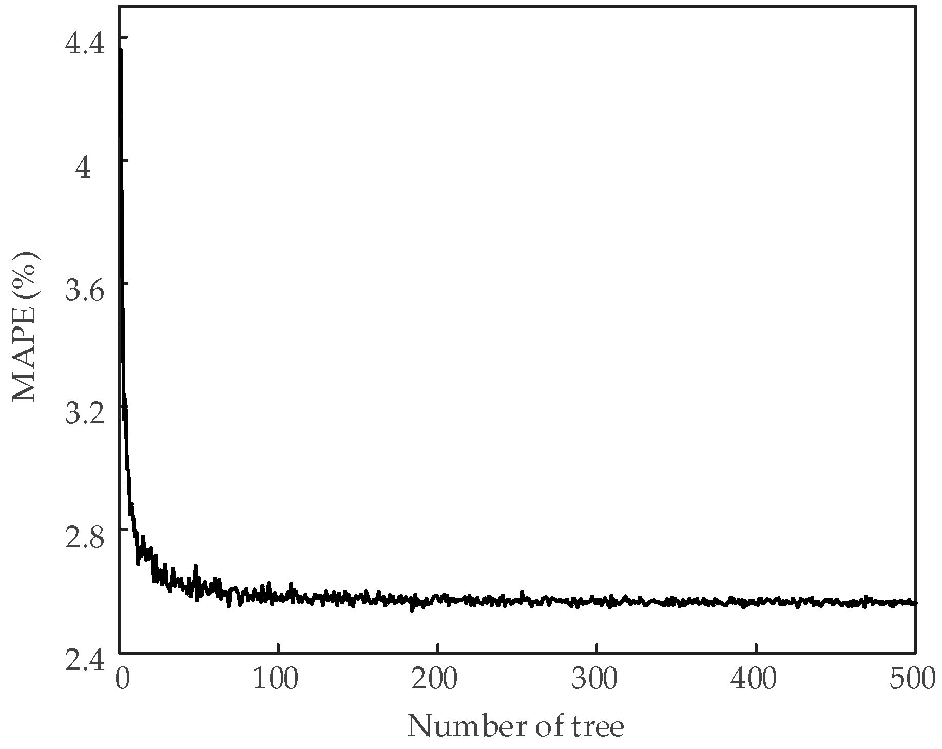
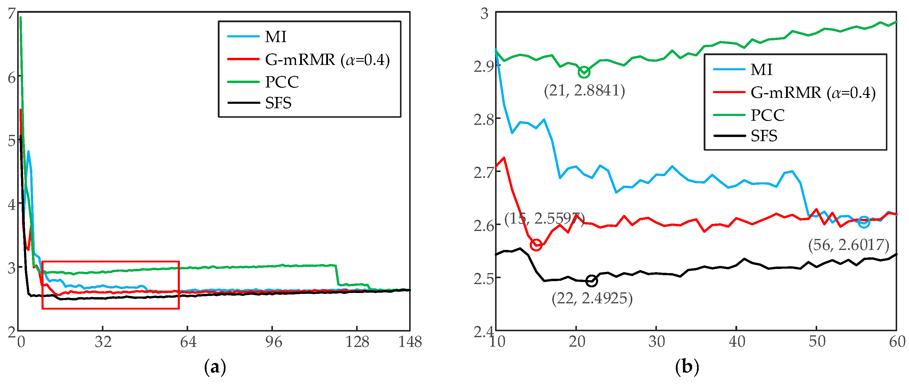
5.1. Feature Selection Results Based on G-mRMR and RF
- (1)
- The training set and test set with optimal features are used for the experiment.
- (2)
- The initial number of tree nTree = 1.
- (3)
- Training RF and testing with different nTree value with increment of 1 until nTree = 500.
5.2. Comparison Experiments for STLF
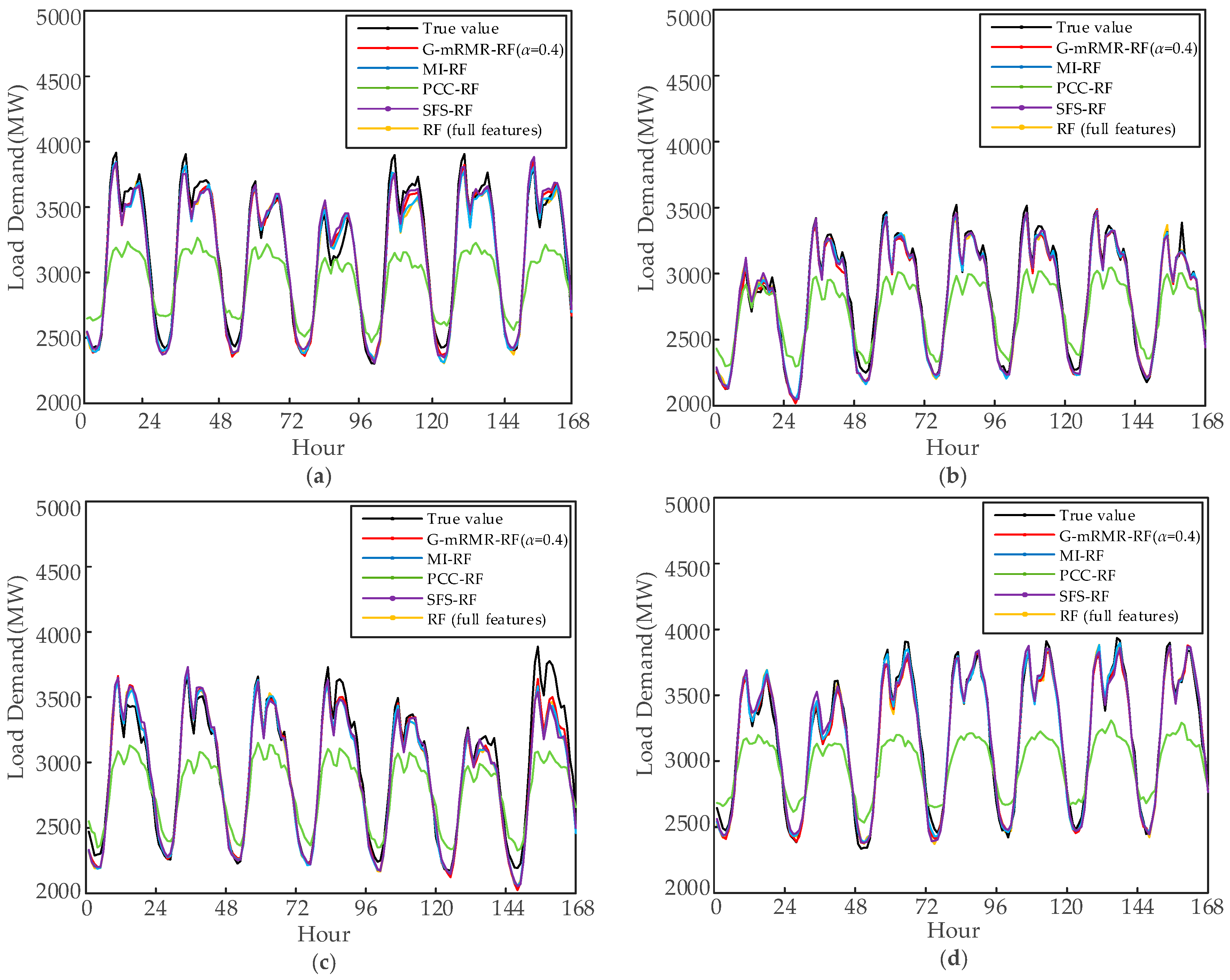
5.2.1. Comparison of Different Feature Selection Methods
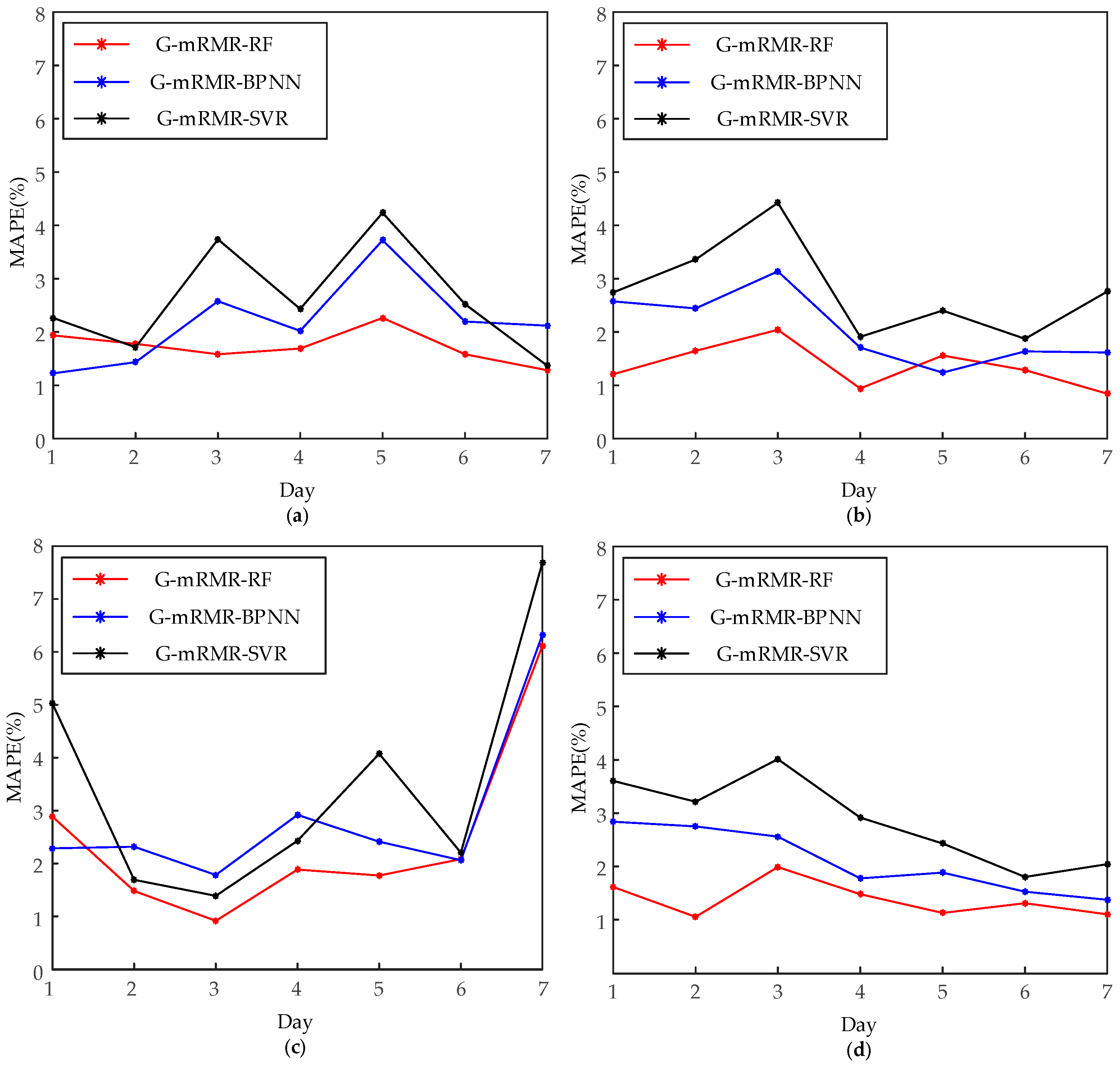
5.2.2. Comparison of Different Intelligent Methods
6. Conclusions
- (1)
- MI is adopted as the criterion to measure the relevance between features and time series of load and the dependency among features, which is the basis of quantitative analysis of feature selection by mRMR.
- (2)
- The correlation between features and load as well as the redundancy of these features are considered. As compared to the maximum relevance method, the G-mRMR method for feature selection reduces the number of optimal feature subset and avoids the association of STLF accuracy with the redundancy of features. For the time being, the relevance and redundancy are balanced by using a variable weighting factor. The features selected by G-mRMR make the accuracy of RF more precise than mRMR.
- (3)
- The optimal structure of RF is designed for reducing the complexity of the model and for improving the accuracy of STLF.
Acknowledgments
Author Contributions
Conflicts of Interest
References
- Moslehi, K.; Kumar, R. A reliability perspective of the smart grid. IEEE Trans. Smart Grid 2010, 1, 57–64. [Google Scholar] [CrossRef]
- Ren, Y.; Suganthan, P.N.; Srikanth, N.; Amaratunga, G. Random vector functional link network for short-term electricity load demand forecasting. Inf. Sci. 2016, 367–368, 1078–1093. [Google Scholar] [CrossRef]
- Lee, C.-M.; Ko, C.-N. Short-term load forecasting using lifting scheme and ARIMA models. Expert Syst. Appl. 2011, 38, 5902–5911. [Google Scholar] [CrossRef]
- Goia, A.; May, C.; Fusai, G. Functional clustering and linear regression for peak load forecasting. Int. J. Fofrecast. 2010, 26, 700–711. [Google Scholar] [CrossRef]
- Al-Hamadi, H.M.; Soliman, S.A. Fuzzy short-term electric load forecasting using Kalman filter. IEE Proc. Gener. Transm. Distrib. 2006, 153, 217–227. [Google Scholar] [CrossRef]
- Ramos, S.; Soares, J.; Vale, Z. Short-term load forecasting based on load profiling. In Proceedings of the 2013 IEEE Power and Energy Society General Meeting, Vancouver, BC, Canada, 21–25 July 2013; pp. 1–5.
- Li, W.; Zhang, Z.G. Based on Time Sequence of ARIMA Model in the Application of Short-Term Electricity Load Forecasting. In Proceedings of the 2009 International Conference on Research Challenges in Computer Science, Shanghai, China, 28–29 December 2009; pp. 11–14.
- Deshmukh, M.R.; Mahor, A. Comparisons of Short Term Load Forecasting using Artificial Neural Network and Regression Method. Int. J. Adv. Comput. Res. 2011, 1, 96–100. [Google Scholar]
- Taylor, J.W. Short-Term Load Forecasting With Exponentially Weighted Methods. IEEE Trans. Power Syst. 2012, 27, 458–464. [Google Scholar] [CrossRef]
- Kouhi, S.; Keynia, F.; Ravadanegh, S.N. A new short-term load forecast method based on neuro-evolutionary algorithm and chaotic feature selection. Int. J. Electr. Power Energy Syst. 2014, 62, 862–867. [Google Scholar] [CrossRef]
- Raza, M.Q.; Khosravi, A. A review on artificial intelligence based load demand forecasting techniques for smart grid and buildings. Renew. Sustain. Energy Rev. 2015, 50, 1352–1372. [Google Scholar] [CrossRef]
- Lin, C.T.; Chou, L.D.; Chen, Y.M.; Tseng, L.M. A hybrid economic indices based short-term load forecasting system. Int. J. Electr. Power Energy Syst. 2014, 54, 293–305. [Google Scholar] [CrossRef]
- Yu, F.; Xu, X. A short-term load forecasting model of natural gas based on optimized genetic algorithm and improved BP neural network. Appl. Energy 2014, 134, 102–113. [Google Scholar] [CrossRef]
- Çevik, H.H.; Çunkaş, M. Short-term load forecasting using fuzzy logic and ANFIS. Neural Comput. Appl. 2015, 26, 1355–1367. [Google Scholar] [CrossRef]
- Lahouar, A.; Slama, J.B.H. Day-ahead load forecast using random forest and expert input selection. Energy Convers. Manag. 2015, 103, 1040–1051. [Google Scholar] [CrossRef]
- Ho, K.L.; Hsu, Y.Y.; Chen, C.F.; Lee, T.E. Short term load forecasting of Taiwan power system using a knowledge-based expert system. IEEE Trans. Power Syst. 1990, 5, 1214–1221. [Google Scholar]
- Srinivasan, D.; Tan, S.S.; Cheng, C.S.; Chan, E.K. Parallel neural network-fuzzy expert system strategy for short-term load forecasting: System implementation and performance evaluation. IEEE Trans. Power Syst. 1999, 14, 1100–1106. [Google Scholar] [CrossRef]
- Quan, H.; Srinivasan, D.; Khosravi, A. Uncertainty handling using neural network-based prediction intervals for electrical load forecasting. Energy 2014, 73, 916–925. [Google Scholar] [CrossRef]
- Hernández, L.; Baladrón, C.; Aguiar, J.M.; Carro, B.; Sánchez-Esguevillas, A.; Lloret, J. Artificial neural networks for short-term load forecasting in microgrids environment. Energy 2014, 75, 252–264. [Google Scholar] [CrossRef]
- Ko, C.N.; Lee, C.M. Short-term load forecasting using SVR (support vector regression)-based radial basis function neural network with dual extended Kalman filter. Energy 2013, 49, 413–422. [Google Scholar] [CrossRef]
- Che, J.X.; Wang, J.Z. Short-term load forecasting using a kernel-based support vector regression combination model. Appl. Energy 2014, 132, 602–609. [Google Scholar] [CrossRef]
- Pandian, S.C.; Duraiswamy, K.; Rajan, C.C.A.; Kanagaraj, N. Fuzzy approach for short term load forecasting. Electr. Power Syst. Res. 2006, 76, 541–548. [Google Scholar] [CrossRef]
- Božić, M.; Stojanović, M.; Stajić, Z.; Stajić, N. Mutual Information-Based Inputs Selection for Electric Load Time Series Forecasting. Entropy 2013, 15, 926–942. [Google Scholar] [CrossRef]
- Ma, L.; Zhou, S.; Lin, M. Support Vector Machine Optimized with Genetic Algorithm for Short-Term Load Forecasting. In Proceedings of the 2008 International Symposium on Knowledge Acquisition and Modeling, Wuhan, China, 21–22 December 2008; pp. 654–657.
- Gao, R.; Liu, X. Support vector machine with PSO algorithm in short-term load forecasting. In Proceedings of the 2008 Chinese Control and Decision Conference, Yantai, China, 2–4 July 2008; pp. 1140–1142.
- Breiman, L. Random Forests. Mach. Learn. 2001, 45, 5–32. [Google Scholar] [CrossRef]
- Jurado, S.; Nebot, À.; Mugica, F.; Avellana, N. Hybrid methodologies for electricity load forecasting: Entropy-based feature selection with machine learning and soft computing techniques. Energy 2015, 86, 276–291. [Google Scholar] [CrossRef] [Green Version]
- Wilamowski, B.M.; Cecati, C.; Kolbusz, J.; Rozycki, P. A Novel RBF Training Algorithm for short-term Electric Load Forecasting and Comparative Studies. IEEE Trans. Ind. Electron. 2015, 62, 6519–6529. [Google Scholar]
- Wi, Y.M.; Joo, S.K.; Song, K.B. Holiday load forecasting using fuzzy polynomial regression with weather feature selection and adjustment. IEEE Trans. Power Syst. 2012, 27, 596–603. [Google Scholar] [CrossRef]
- Viegas, J.L.; Vieira, S.M.; Melício, M.; Mendes, V.M.F.; Sousa, J.M.C. GA-ANN Short-Term Electricity Load Forecasting. In Proceedings of the 7th IFIP WG 5.5/SOCOLNET Advanced Doctoral Conference on Computing, Electrical and Industrial Systems, Costa de Caparica, Portugal, 11–13 April 2016; pp. 485–493.
- Li, S.; Wang, P.; Goel, L. A novel wavelet-based ensemble method for short-term load forecasting with hybrid neural networks and feature selection. IEEE Trans. Power Syst. 2015, 1788–1798. [Google Scholar] [CrossRef]
- Hu, Z.; Bao, Y.; Chiong, R.; Xiong, T. Mid-term interval load forecasting using multi-output support vector regression with a memetic algorithm for feature selection. Energy 2015, 84, 419–431. [Google Scholar] [CrossRef]
- Koprinska, I.; Rana, M.; Agelidis, V.G. Yearly and seasonal models for electricity load forecasting. In Proceedings of the 2011 International Joint Conference on Neural Networks (IJCNN), San Jose, CA, USA, 31 July–5 August 2011; pp. 1474–1481.
- Peng, H.; Long, F.; Ding, C. Feature selection based on mutual information: Criteria of max-dependency, max-relevance, and min-redundancy. IEEE Trans. Pattern Anal. Mach. Intell. 2005, 27, 1226–1238. [Google Scholar] [CrossRef] [PubMed]
- Nguyen, X.V.; Chan, J.; Romano, S.; Bailey, J. Effective global approaches for mutual information based feature selection. In Proceedings of the 20th ACM SIGKDD International Conference on Knowledge Discovery and Data Mining, New York, NY, USA, 24–27 August 2014; pp. 512–521.
- Speybroeck, N. Classification and regression trees. Int. J. Public Health 2012, 57, 243–246. [Google Scholar] [CrossRef] [PubMed]
- Breiman, L. Bagging predictors. Mach. Learn. 1996, 24, 123–140. [Google Scholar] [CrossRef]
- Sood, R.; Koprinska, I.; Agelidis, V.G. Electricity load forecasting based on autocorrelation analysis. In Proceedings of the 2010 International Joint Conference on Neural Networks (IJCNN), Barcelona, Spain, 18–23 July 2010; pp. 1–8.
- Kohavi, R.; John, G.H. Wrappers for feature subset selection. Artif. Intell. 1997, 97, 273–324. [Google Scholar] [CrossRef]
- Dudek, G. Short-Term Load Forecasting Using Random Forests. In Intelligent Systems’2014; Springer: Cham, Switzerland, 2015; pp. 821–828. [Google Scholar]
- Che, J.X.; Wang, J.Z.; Tang, Y.J. Optimal training subset in a support vector regression electric load forecasting model. Appl. Soft Comput. 2012, 12, 1523–1531. [Google Scholar] [CrossRef]
- Sheela, K.G.; Deepa, S.N. Review on Methods to Fix Number of Hidden Neurons in Neural Networks. Math. Probl. Eng. 2013, 2013, 425740. [Google Scholar] [CrossRef]
- Rana, M.; Koprinska, I. Forecasting electricity load with advanced wavelet neural networks. Neurocomputing 2016, 182, 118–132. [Google Scholar] [CrossRef]


| Feature Type | Original Feature |
|---|---|
| Exogenous features | 1.FHour, 2.FWW, 3.FDW, 4.FS |
| Endogenous features | 5.FL(t-25), 6.FL(t-26), 7.FL(t-27), 8.FL(t-28), …, 146.FL(t-166), 147.FL(t-167), 148.FL(t-168) |
| Data Set | Information | Purpose |
|---|---|---|
| Training Set | January, February, May, June, August, September, October, December | Train RF |
| Validation Set | March, April, July, November | Use for obtain the best weighting factor |
| Test Set | 23–29 February 2012 (Winter) 13–19 May 2012 (Spring) 21–27 August 2012 (Summer) 24–30 November 2012 (Fall) | Test performance of RF |
| α | Min MAPE (%) | Number of Features | Feature Subset |
|---|---|---|---|
| 0.1 | 2.5640 | 26 | FL(t-168), FL(t-25), FL(t-48), FL(t-144), FL(t-72), FHour, FL(t-47), FL(t-26), FL(t-120), FL(t-167), FWW, FS, FDW, FL(t-34), FL(t-158), FL(t-103), FL(t-27), FL(t-96), FL(t-162), FL(t-132), FL(t-44), FL(t-88), FL(t-149), FL(t-153), FL(t-37), FL(t-107) |
| 0.2 | 2.5857 | 25 | FL(t-168), FL(t-25), FL(t-48), FL(t-144), FHour, FS, FWW, FL(t-71), FDW, FL(t-27), FL(t-106), FL(t-162), FL(t-38), FL(t-127), FL(t-93), FL(t-156), FL(t-88), FL(t-32), FL(t-29), FL(t-96), FL(t-44), FL(t-134), FL(t-26), FL(t-166), FL(t-59) |
| 0.3 | 2.5858 | 27 | FL(t-168), FL(t-25), FL(t-48), FHour, FWW, FS, FL(t-144), FDW, FL(t-103), FL(t-37), FL(t-162), FL(t-70), FL(t-131), FL(t-28), FL(t-88), FL(t-153), FL(t-106), FL(t-75), FL(t-159), FL(t-34), FL(t-125), FL(t-96), FL(t-43), FL(t-165), FL(t-109), FL(t-31), FL(t-26) |
| 0.4 | 2.5597 | 15 | FL(t-168), FL(t-25), FL(t-48), FWW, FS, FL(t-127), FL(t-85), FL(t-139), FDW, FL(t-34), FL(t-160), FL(t-70), FL(t-28), FL(t-120), FL(t-141) |
| 0.5 | 2.5897 | 80 | FL(t-168), FL(t-25), FL(t-47), FWW, FS, FL(t-127), FL(t-86), FDW, FL(t-139), FL(t-35), FL(t-99), FL(t-160), FL(t-69), FL(t-29), FL(t-154), FL(t-120), FL(t-41), FL(t-81), FL(t-133), FL(t-148), FL(t-166), FL(t-32), FL(t-63), FL(t-92), FL(t-26), FL(t-108), FL(t-162), FL(t-78), … |
| 0.6 | 2.5868 | 46 | FL(t-168), FL(t-25), FHour, FL(t-47), FS, FL(t-127), FL(t-88), FDW, FL(t-156), FL(t-139), FL(t-76), FL(t-34), FL(t-110), FL(t-69), FL(t-149), FL(t-120), FL(t-41), FL(t-81), FL(t-27), FL(t-165), FL(t-37), FL(t-162), FL(t-98), FL(t-30), FL(t-131), FL(t-159), FL(t-104), FL(t-44), … |
| 0.7 | 2.5891 | 88 | FL(t-168), FL(t-25), FWW, FS, FL(t-103), FL(t-61), FL(t-139), FDW, FL(t-47), FL(t-160), FL(t-82), FL(t-124), FL(t-30), FL(t-93), FL(t-156), FL(t-41), FL(t-146), FL(t-33), FL(t-110), FL(t-72), FL(t-152), FL(t-164), FL(t-27), FL(t-90), FL(t-131), FL(t-39), FL(t-118), FL(t-77), … |
| 0.8 | 2.6046 | 93 | FL(t-168), FL(t-25), FWW, FS, FL(t-103), FL(t-61), FL(t-139), FDW, FL(t-47), FL(t-160), FL(t-82), FL(t-124), FL(t-30), FL(t-93), FL(t-156), FL(t-41), FL(t-146), FL(t-33), FL(t-110), FL(t-166), FL(t-75), FL(t-152), FL(t-90), FL(t-72), FL(t-44), FL(t-131), FL(t-28), FL(t-39), … |
| 0.9 | 2.5918 | 35 | FL(t-168), FL(t-25), FWW, FS, FL(t-103), FL(t-67), FL(t-133), FDW, FL(t-34), FL(t-160), FL(t-46), FL(t-148), FL(t-96), FL(t-29), FL(t-84), FL(t-140), FL(t-39), FL(t-153), FL(t-75), FL(t-114), FL(t-165), FL(t-56), FL(t-122), FL(t-62), FL(t-155), FL(t-126), FL(t-41), FL(t-119), … |
| Day | G-mRMR-RF (α = 0.4) | MI-RF | PCC-RF | SFS-RF | RF with Full Features | |||||
|---|---|---|---|---|---|---|---|---|---|---|
| MAPE | RMSE | MAPE | RMSE | MAPE | RMSE | MAPE | RMSE | MAPE | RMSE | |
| Day 1 | 1.93 | 75.24 | 1.79 | 69.42 | 10.28 | 401.01 | 2.07 | 79.58 | 1.91 | 70.74 |
| Day 2 | 1.77 | 66.63 | 1.78 | 67.90 | 9.78 | 388.26 | 2.22 | 79.46 | 1.80 | 69.13 |
| Day 3 | 1.58 | 53.24 | 1.63 | 51.63 | 7.59 | 285.51 | 1.47 | 49.33 | 1.50 | 50.49 |
| Day 4 | 1.69 | 79.28 | 1.59 | 70.02 | 5.35 | 189.65 | 2.52 | 105.32 | 1.98 | 76.33 |
| Day 5 | 2.26 | 90.72 | 2.66 | 104.16 | 11.14 | 440.91 | 2.04 | 83.68 | 2.91 | 113.32 |
| Day 6 | 1.58 | 57.73 | 2.37 | 83.87 | 9.78 | 396.44 | 1.61 | 57.41 | 2.54 | 87.59 |
| Day 7 | 1.28 | 51.92 | 0.97 | 36.35 | 9.26 | 362.46 | 1.87 | 73.03 | 1.29 | 44.60 |
| Average | 1.72 | 67.82 | 1.82 | 69.05 | 9.02 | 352.03 | 1.97 | 75.40 | 1.99 | 73.17 |
| Day | G-mRMR-RF (α = 0.4) | MI-RF | PCC-RF | SFS-RF | RF with Full Features | |||||
|---|---|---|---|---|---|---|---|---|---|---|
| MAPE | RMSE | MAPE | RMSE | MAPE | RMSE | MAPE | RMSE | MAPE | RMSE | |
| Day 1 | 1.20 | 42.36 | 1.22 | 39.15 | 3.76 | 110.39 | 1.43 | 50.90 | 1.57 | 47.92 |
| Day 2 | 1.64 | 60.32 | 1.33 | 50.26 | 8.98 | 273.78 | 1.28 | 46.10 | 1.37 | 53.34 |
| Day 3 | 2.04 | 66.88 | 2.04 | 67.09 | 6.56 | 246.64 | 2.03 | 69.43 | 2.00 | 66.78 |
| Day 4 | 0.94 | 34.38 | 0.96 | 34.48 | 7.04 | 263.29 | 0.89 | 34.98 | 1.11 | 41.54 |
| Day 5 | 1.55 | 53.26 | 1.40 | 46.62 | 7.17 | 261.54 | 1.40 | 50.04 | 1.50 | 52.38 |
| Day 6 | 1.28 | 41.45 | 1.34 | 44.68 | 6.66 | 237.55 | 1.28 | 40.22 | 1.45 | 40.03 |
| Day 7 | 0.84 | 26.82 | 0.99 | 36.97 | 5.51 | 178.83 | 0.92 | 50.61 | 1.01 | 49.05 |
| Average | 1.35 | 46.49 | 1.33 | 48.03 | 6.53 | 224.57 | 1.32 | 48.90 | 1.40 | 50.15 |
| Day | G-mRMR-RF (α = 0.4) | MI-RF | PCC-RF | SFS-RF | RF with Full Features | |||||
|---|---|---|---|---|---|---|---|---|---|---|
| MAPE | RMSE | MAPE | RMSE | MAPE | RMSE | MAPE | RMSE | MAPE | RMSE | |
| Day 1 | 2.88 | 92.71 | 2.61 | 83.05 | 6.69 | 258.31 | 3.32 | 104.41 | 2.89 | 90.68 |
| Day 2 | 1.48 | 55.30 | 1.55 | 56.81 | 8.22 | 319.74 | 1.77 | 62.53 | 1.59 | 57.62 |
| Day 3 | 0.91 | 31.93 | 0.82 | 29.02 | 7.04 | 263.33 | 1.00 | 38.68 | 1.07 | 36.28 |
| Day 4 | 1.88 | 76.95 | 2.27 | 90.86 | 8.97 | 344.82 | 1.99 | 84.88 | 2.17 | 87.44 |
| Day 5 | 1.77 | 54.77 | 1.87 | 56.56 | 6.42 | 227.25 | 2.16 | 70.95 | 1.91 | 58.15 |
| Day 6 | 2.08 | 73.60 | 1.78 | 71.44 | 5.91 | 181.33 | 1.71 | 65.13 | 1.86 | 74.78 |
| Day 7 | 6.12 | 208.00 | 6.77 | 237.00 | 11.26 | 458.19 | 6.98 | 247.66 | 6.57 | 227.17 |
| Average | 2.45 | 72.83 | 2.52 | 89.25 | 7.79 | 293.28 | 2.70 | 96.32 | 2.58 | 90.30 |
| Day | G-mRMR-RF (α = 0.4) | MI-RF | PCC-RF | SFS-RF | RF with Full Features | |||||
|---|---|---|---|---|---|---|---|---|---|---|
| MAPE | RMSE | MAPE | RMSE | MAPE | RMSE | MAPE | RMSE | MAPE | RMSE | |
| Day 1 | 1.61 | 58.60 | 1.64 | 58.26 | 6.80 | 263.40 | 1.96 | 68.90 | 1.78 | 63.62 |
| Day 2 | 1.05 | 48.24 | 1.12 | 43.26 | 6.97 | 242.74 | 2.11 | 78.43 | 1.09 | 40.30 |
| Day 3 | 1.98 | 74.62 | 2.06 | 74.67 | 10.78 | 427.39 | 1.98 | 73.90 | 2.12 | 76.64 |
| Day 4 | 1.47 | 57.14 | 1.33 | 48.09 | 9.21 | 387.30 | 1.80 | 67.13 | 1.50 | 57.63 |
| Day 5 | 1.12 | 42.84 | 0.90 | 33.83 | 10.29 | 413.17 | 1.15 | 46.87 | 1.26 | 45.01 |
| Day 6 | 1.31 | 53.79 | 1.33 | 52.33 | 9.03 | 389.52 | 1.32 | 54.74 | 1.23 | 47.40 |
| Day 7 | 1.10 | 42.86 | 1.22 | 45.31 | 9.53 | 387.69 | 1.06 | 44.21 | 1.18 | 43.42 |
| Average | 1.38 | 54.01 | 1.37 | 50.82 | 8.93 | 358.74 | 1.63 | 62.02 | 1.45 | 53.43 |
| Predictor | Min MAPE (%) | Number of Features | Feature Subset |
|---|---|---|---|
| G-mRMR-RF (α = 0.4) | 2.5389% | 15 | FL(t-168), FL(t-25), FL(t-48), FWW, FS, FL(t-127), FL(t-85), FL(t-139), FDW, FL(t-34), FL(t-160), FL(t-70), FL(t-28), FL(t-120), FL(t-141) |
| G-mRMR-SVR (α = 0.3) | 3.3293% | 5 | FL(t-168), FL(t-25), FL(t-48), FHour, FWW |
| G-mRMR-BPNN (α = 0.1) | 2.7186% | 11 | FL(t-168), FL(t-25), FL(t-48), FL(t-144), FL(t-72), FHour, FL(t-47), FL(t-26), FL(t-120), FL(t-167), FWW |
| Test Set | MAPE (%) | G-mRMR-RF | G-mRMR-ANN | G-mRMR-SVR |
|---|---|---|---|---|
| 23–29 February 2012 (Winter) | Max | 2.26 | 3.72 | 4.24 |
| Min | 1.28 | 1.23 | 1.37 | |
| Ave | 1.72 | 2.18 | 2.61 | |
| 13–19 May 2012 (Spring) | Max | 2.04 | 3.14 | 4.42 |
| Min | 0.84 | 1.24 | 1.87 | |
| Ave | 1.35 | 2.05 | 2.78 | |
| 21–27 August 2012 (Summer) | Max | 6.12 | 6.32 | 7.68 |
| Min | 0.91 | 1.78 | 1.69 | |
| Ave | 2.45 | 2.87 | 3.50 | |
| 24–30 November 2012 (Fall) | Max | 1.98 | 2.84 | 4.01 |
| Min | 1.05 | 1.38 | 1.80 | |
| Ave | 1.38 | 2.10 | 2.86 |
© 2016 by the authors; licensee MDPI, Basel, Switzerland. This article is an open access article distributed under the terms and conditions of the Creative Commons Attribution (CC-BY) license (http://creativecommons.org/licenses/by/4.0/).
Share and Cite
Huang, N.; Hu, Z.; Cai, G.; Yang, D. Short Term Electrical Load Forecasting Using Mutual Information Based Feature Selection with Generalized Minimum-Redundancy and Maximum-Relevance Criteria. Entropy 2016, 18, 330. https://doi.org/10.3390/e18090330
Huang N, Hu Z, Cai G, Yang D. Short Term Electrical Load Forecasting Using Mutual Information Based Feature Selection with Generalized Minimum-Redundancy and Maximum-Relevance Criteria. Entropy. 2016; 18(9):330. https://doi.org/10.3390/e18090330
Chicago/Turabian StyleHuang, Nantian, Zhiqiang Hu, Guowei Cai, and Dongfeng Yang. 2016. "Short Term Electrical Load Forecasting Using Mutual Information Based Feature Selection with Generalized Minimum-Redundancy and Maximum-Relevance Criteria" Entropy 18, no. 9: 330. https://doi.org/10.3390/e18090330