Article

Entropy Minimizing Curves with Application to Flight Path Design and Clustering †

by
Stéphane Puechmorel
* and
Florence Nicol
Laboratoire de Mathématiques Appliquées, Informatique et Automatique pour l’Aérien (MAIAA), Département Sciences et Ingénierie de la Navigation Aérienne (SINA), École Nationale de l’Aviation Civile (ENAC), 7 avenue Edouard Belin CS 54005, 31055 Toulouse, France
*
Author to whom correspondence should be addressed.
This paper is an extended version of our paper published in the 2nd Conference on Geometric Science of Information, Paris, France, 28–30 October 2015.
Entropy 2016, 18(9), 337; https://doi.org/10.3390/e18090337
Submission received: 26 July 2016 / Revised: 8 September 2016 / Accepted: 8 September 2016 / Published: 15 September 2016
(This article belongs to the Special Issue Differential Geometrical Theory of Statistics)

Abstract

:
Air traffic management (ATM) aims at providing companies with a safe and ideally optimal aircraft trajectory planning. Air traffic controllers act on flight paths in such a way that no pair of aircraft come closer than the regulatory separation norms. With the increase of traffic, it is expected that the system will reach its limits in the near future: a paradigm change in ATM is planned with the introduction of trajectory-based operations. In this context, sets of well-separated flight paths are computed in advance, tremendously reducing the number of unsafe situations that must be dealt with by controllers. Unfortunately, automated tools used to generate such planning generally issue trajectories not complying with operational practices or even flight dynamics. In this paper, a means of producing realistic air routes from the output of an automated trajectory design tool is investigated. For that purpose, the entropy of a system of curves is first defined, and a mean of iteratively minimizing it is presented. The resulting curves form a route network that is suitable for use in a semi-automated ATM system with human in the loop. The tool introduced in this work is quite versatile and may be applied also to unsupervised classification of curves: an example is given for French traffic.

1. Introduction

Based on recent studies [1], traffic in Europe is expected to grow by an average yearly rate of 2.6%, yielding a net increase of two million flights per year at the 2020 horizon. The long-term forecast gives a two-fold increase in 2050 over the current traffic, pointing out the need for a paradigm change in the way flights are managed. Two major framework programs, SESAR (Single European Sky Air traffic management Research) in Europe and Nextgen in the U.S. have been launched in order to first investigate potential solutions and to deploy them in a second phase. One of the main changes that the air traffic management (ATM) system will undergo is a switch from airspace-based to trajectory-based operations with a delegation of the separation task to the crews. Within this framework, trajectories become the basic object of ATM, changing the way air traffic controllers will be working. In order to alleviate the workload of controllers, trajectories will be planned several weeks in advance in such a way that close encounters are minimized and ideally removed. For that purpose, several tools are currently being developed; most of them coming from the field of robotics [2]. Unfortunately, flight paths issued by these algorithms are not tractable for a human controller and need to be simplified. The purpose of the present work is to introduce an automated procedure that takes as input a set of trajectories and outputs a simplified one that can be used in an operational context. Please note that the separation norm constraints were not taken into account in this work. In our algorithm, we cannot enforce the regulatory separation norms, just construct clusters with low interactions. According to the applications, the results of our algorithm may be used as an initial solution of a post-processing algorithm based on optimal control in order to keep in line with the regulatory constraints. Using entropy associated with a curves system, a gradient descent is performed in order to reduce it so as to straighten trajectories while avoiding areas with low aircraft density, thus enforcing route-like behavior. This effect is related to the fact that entropy-minimizing distributions favor concentration.

2. Entropy-Minimizing Curves

2.1. Motivation

As previously mentioned, air traffic management of the future will make an intensive use of 4D trajectories as a basic object. Full automation is a far-reaching concept that will probably not be implemented before 2040–2050, and even in such a situation, it will be necessary to keep humans in the loop so as to gain a wide societal acceptance of the concept. Starting from SESAR or Nextgen initial deployment and aiming towards this ultimate objective, a transition phase with human-system cooperation will take place. Since ATC controllers are used to a well-structured network of routes, it is advisable to post-process the 4D trajectories issued by automated systems in order to make them as close as possible to line segments connecting beacons. To perform this task, in an automatic way, flight paths will be deformed so as to minimize an entropy criterion that enforces avoidance of low density areas and at the same time penalizes length. Compared to already available bundling algorithms [3] that tend to move curves to high density areas, this new procedure generates geometrically-correct curves, without excess curvature.
Let a set γ 1 , , γ N of smooth curves be given that will be aircraft flight paths for the air traffic application. It will be assumed in the sequel that all curves are smooth mappings from [ 0 , 1 ] to a domain Ω of R q with everywhere non-vanishing derivatives in ] 0 , 1 [ . This last condition allows one to view them as smooth immersions with boundaries and is sound from the application point of view, as aircraft velocities are bounded below by the efficiency consideration and ultimately by the stall and, therefore, cannot vanish expect at the endpoints. In air traffic applications, the dimension of the state space is generally two and sometimes three when the evolution of the aircraft in the vertical plane is of interest.
The approach taken in this work is first to get a sound definition of spatial density associated with a curve system, then to derive from it an entropy that will be minimized.

2.2. Spatial Density of a System of Curves

Due to the fact that aircraft positions are acquired through radar measurements, a trajectory is known only at discrete sampling times. In the operational context, the sampling period ranges from 4 to 10 s, which corresponds roughly to a 100–250-m traveling distance. Derived from that, a classical performance indicator used in ATM is the aircraft density [4], obtained from the sampled positions γ i ( t j ) , j = 1 , , n i on each flight path γ i , i = 1 , , N . It is constructed from a partition U k , k = 1 , , P of Ω by counting the number of samples occurring in a given U k , then dividing out by the total number of samples n = i = 1 N n i . More formally, the density d k in the subset U k of Ω is expressed as:
d k = n 1 i = 1 N j = 1 n i 1 U k γ i ( t j )
with 1 U k the characteristic function of the set U k . It seems natural to extend the density obtained from samples to another one based on the trajectories themselves using an integral form:
d k = λ 1 i = 1 N 0 1 1 U k γ i ( t ) d t
where the normalizing constant λ is chosen so that d k is a discrete probability distribution:
λ = k = 1 P i = 1 N 0 1 1 U k γ i ( t ) d t = i = 1 N 0 1 k = 1 P 1 U k γ i ( t ) d t
and since U k , k = 1 , , P is a partition:
k = 1 P 1 U k γ i ( t ) = 1
so that λ = N .
Density can be viewed as an empirical probability distribution with the U k considered as bins in an histogram. It is thus natural to extend the above computation so as to give rise to a continuous distribution on Ω. For that purpose, local weighting techniques, such as kernel density estimation methods, are well known in nonparametric statistics, because they are a useful data-driven way to yield continuous density estimation. Many references may be found in the literature as in [5,6]. Given the observations, the resulting estimation will be the sum of weights taking into account the distance between the observations and the location x at which the density has to be estimated; the more an observation is close to x, the greater is the weighting. The weights are defined by selecting a summable function centered on the observations, called a kernel, usually denoted by K : R R + in the univariate case, and a smoothed version of the Parzen–Rosenblatt density estimator [7,8] is used. Standard choices for the K function are the ones used for nonparametric kernel estimation, like the Epanechnikov function [9]:
K : x 1 x 2 1 [ 1 , 1 ] ( x ) .
There exists a large variety of kernel functions, and any density function satisfying the normalization condition can be considered, so that the estimation is a probability density. Moreover, the kernel function is a symmetric positive function, with the first moment equal to zero and a finite second order moment. In the multivariate case, a multivariate kernel function K : R q R + is selected that can be expressed by means of a real kernel K associated with a norm, denoted by . , in R q as follows:
K ( x ) = K ( x ) , x R q .
The normalization condition becomes:
R q K x d x = R q K x d x = 1 .
A kernel version of the density is then defined as a mapping d from Ω to [ 0 , 1 ] :
d : x i = 1 N 0 1 K x γ i ( t ) d t i = 1 N Ω 0 1 K x γ i ( t ) d t d x .
Normalizing the kernel is not mandatory, as the normalization occurs with the definition of d. It is nevertheless easier to consider these kinds of kernels, as is done in nonparametric density estimation. Note that when K is compactly supported, which is the case of the Epanechnikov function and all of its relatives, it becomes:
Ω K x γ i ( t ) d x = R q K x d x
provided that Ω contains the set:
{ x R q , inf i = 1 N , t [ 0 , 1 ] x γ i ( t ) A }
where the interval [ A , A ] contains the support of K. The case of kernels with unbounded support, like Gaussian functions, may be dealt with provided Ω = R q . In the application considered, only compactly-supported kernels are used, mainly to allow fast machine implementation of the density computation.
Using the polar coordinates ( ρ , θ ) and the rotation invariance of the integrand, the relation becomes:
V o l S q 1 R + K ( ρ ) ρ q 1 d ρ = 1
which yields a normalizing constant of 2 / π for the Epanechnikov function in dimension two, instead of the usual 3 / 4 in the real case. When the normalization condition is fulfilled, the expression of the density simplifies to:
d : x N 1 i = 1 N 0 1 K x γ i ( t ) d t .
The normalizing constant is the same as in (2).
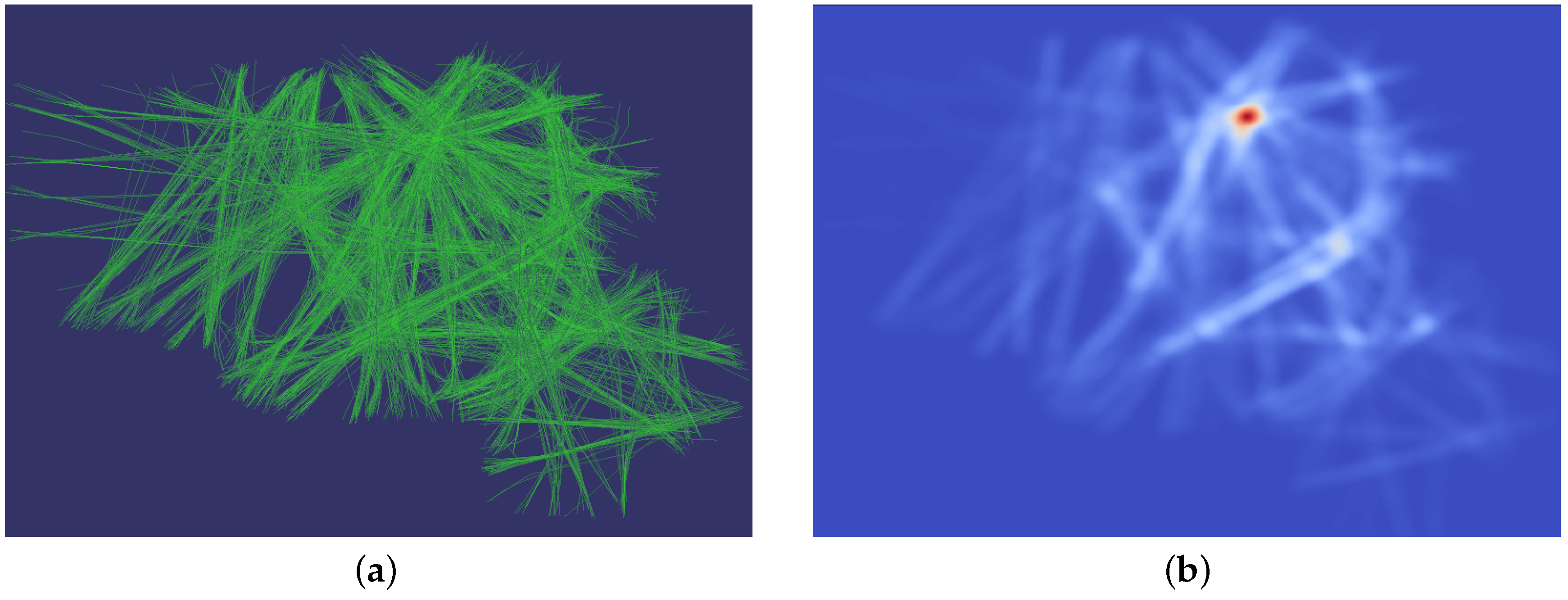
As an example, one day of traffic over France is considered and pictured in Figure 1 with the corresponding density map, computed on an evenly-spaced grid with a normalized Epanechnikov kernel.
Unfortunately, density computed this way suffers a severe flaw for the ATM application: it is not related only to the shape of trajectories, but also to the time behavior. Formally, it is defined on the set Imm [ 0 , 1 ] , R q of smooth immersions from [ 0 , 1 ] to R q while the space of primary interest will be the quotient by smooth diffeomorphisms of the interval [ 0 , 1 ] , Imm [ 0 , 1 ] , R q / Diff ( [ 0 , 1 ] ) . Invariance of the density under the action of Diff ( [ 0 , 1 ] ) is obtained as in [10] by adding a term related to velocity in the integrals. The new definition of d becomes:
d ˜ : x i = 1 N 0 1 K x γ i ( t ) γ i ( t ) d t i = 1 N Ω 0 1 K x γ i ( t ) γ i ( t ) d t d x .
Assuming again a normalized kernel and letting l i be the length of the curve γ i , the expression of the density simplifies to:
d ˜ : x i = 1 N 0 1 K x γ i ( t ) γ i ( t ) d t i = 1 N l i .
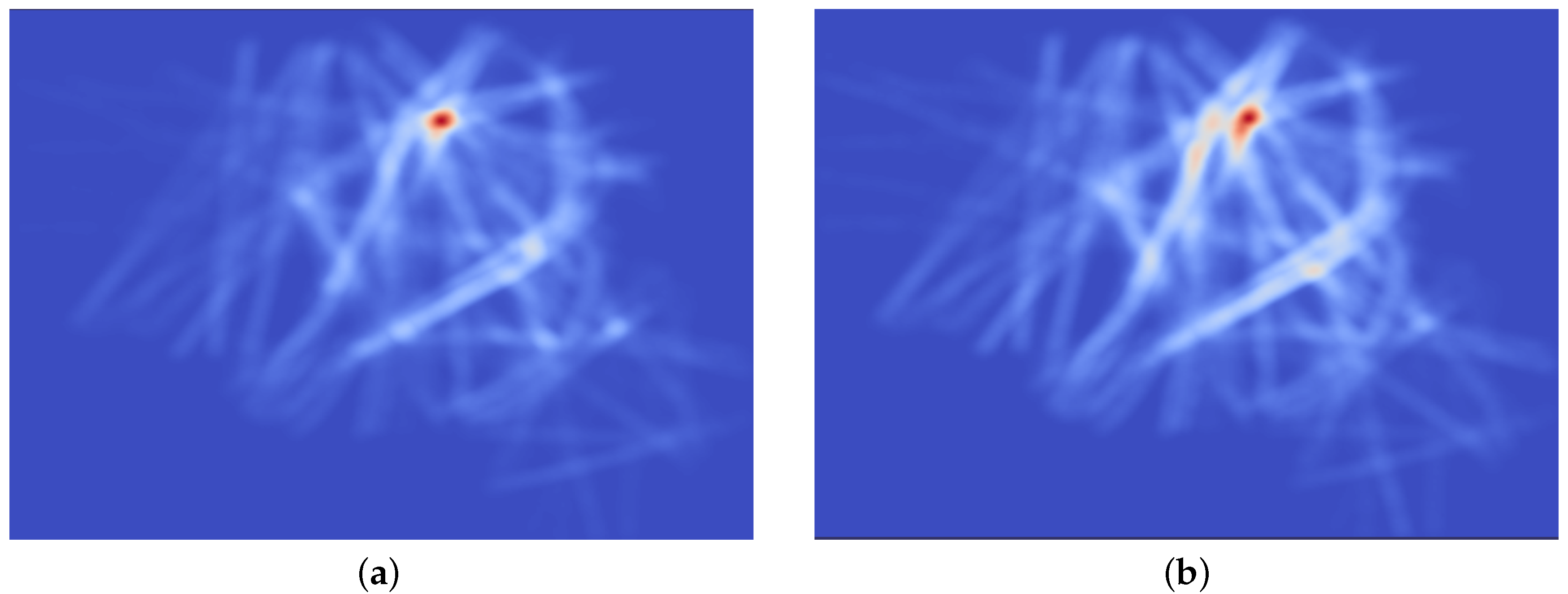
The new Diff-invariant density is pictured in Figure 2 along with the standard density. While the overall aspect of the plot is similar, one can observe that routes are more apparent in the right picture and that the density peak located above the Paris area is of less importance and less symmetric due to the fact that near airports, aircraft are slowing down, and this effect exaggerates the density with the non-invariant definition.
The extension of the two-dimensional defined that way to the general case of curves in an arbitrary space R q is straightforward.

2.3. Further Properties of the Density

In this section, the curves considered are a smooth mapping from the closed interval [ 0 , 1 ] to R q , with a non-vanishing derivative in ] 0 , 1 [ . All multivariate kernels K will be assumed smooth, positive, with a unit integral and of the form x K x . However, it is not required that they are compactly supported unless explicitly stated. All results are presented for the whole space R q , but apply almost verbatim to an open subset.
Definition 1.
Let f be a smooth summable mapping from R to R . The scaling f ν of f is defined, for each ν > 0 , to be the mapping:
f ν : x R 1 ν f x ν .
It is clear that the L 1 -norm of the original mapping is preserved by the scaling. Given a summable kernel function K from R to R + , it defines a multivariate kernel K on R q that maps x to K ( x ) . One may derive from it a parametrized family of kernels in R by mapping each ν in ] 0 , 1 ] to the scaled kernel K ν . If the original K is of unit integral, so are all of the K ν .
Proposition 1.
Let γ : [ 0 , 1 ] R q be a smooth path with a non-vanishing derivative in ] 0 , 1 [ . Let K ν , ν > 0 be a parametrized family of unit integral kernels. The family of Borel measures μ ν defined for any Borel set A by:
μ ν ( A ) = A 0 1 K ν x γ ( t ) γ ( t ) d t d x
is tight and converges narrowly to the Lebesgue measure on γ [ 0 , 1 ] .
Proof. 
Let ϵ > 0 be given. By the summability of K, there exists a positive real number r, such that:
R q B ( 0 , r ) K ( x ) d x < ϵ
with B ( 0 , r ) the open ball of radius r centered at the origin. Since B ( 0 , r ) B ( 0 , r ν 1 ) for ν > 0 , the same holds for all of the family K ν . Let B ( 0 , M ) be an open ball containing γ [ 0 , 1 ] . Then:
μ ν R q B ( 0 , M + r ) ¯ = R q B ( 0 , M + r ) 0 1 K ν x γ ( t ) γ ( t ) d t d x = 0 1 R q B ( 0 , M + r ) K ν x γ ( t ) γ ( t ) d x d t ϵ 0 1 γ ( t ) d t = ϵ l ( γ )
where l ( γ ) denotes the length of γ. This proves the tightness of the family K ν .
Let f : R q R be a bounded continuous mapping. It becomes:
I ν ( f ) = R q 0 1 K ν x γ ( t ) f ( x ) γ ( t ) d t d x = 0 1 R q K ν x γ ( t ) f ( x ) γ ( t ) d x d t = 0 1 R q K x f x ν + γ ( t ) γ ( t ) d x d t
and since f is bounded, the dominated convergence theorem shows that:
lim ν 0 I ν ( f ) = 0 1 f γ ( t ) γ ( t ) d t
proving the second part of the claim. ☐
The density in (7) is for a single curve of the form d ( x ) = l ( γ ) 1 0 1 K x γ ( t ) γ ( t ) d t with l ( γ ) the length of the curve γ. It is invariant under the change of the parameter and can be written in a more concise way as:
0 1 K x γ ( η ) d η
where η is the arclength times l ( γ ) 1 .
This form allows a simple probabilistic interpretation of the density d: if a point u is drawn on the curve γ according to a uniform distribution and independently a vector v in R q with a density K (the multivariate kernel corresponding to K), then the density of x = u + v is given by Equation (10).
Proposition 2.
If the multivariate kernel K has a finite second moment, that is the univariate kernel K is such that:
M = R + r q + 1 K ( r ) d r < +
then the Wasserstein distance between the densities d 1 , d 2 associated with smooth curves γ 1 , γ 2 is bounded by:
2 V o l ( S q 1 ) M + D ( γ 1 , γ 2 )
with :
D ( γ 1 , γ 2 ) = 0 1 γ 1 ( η ) γ 2 ( η ) 2 d η
where each curve is parametrized by the scaled arclength as in (10).
Proof. 
Let us consider the plan [11] given by the density:
d : ( x , y ) 0 1 K ( x γ 1 ( η ) ) K ( y γ 2 ( η ) ) d η
where each curve is parametrized by the scaled arclength. The associated transport cost is given by:
C = R q × R q x y 2 0 1 K x γ 1 ( η ) K y γ 2 ( η ) d η d x d y
letting u = y x and using Fubini gives:
C = 0 1 R q K x γ 1 ( η ) R q u 2 K u + x γ 2 ( η ) d u d x d η .
The inner term can be written as:
R q u 2 K u + x γ 2 ( η ) d u = R q u + γ 2 ( η ) x 2 K u d u = R q u 2 K ( u ) d u + 2 γ 2 ( η ) x , R q u K ( u ) d u + γ 2 ( η ) x 2 .
The integral:
R q u K ( u ) d u
is zero and, using spherical coordinates:
R q u 2 K ( u ) d u = R + r q + 1 K ( r ) S q 1 d σ d r = V o l ( S q 1 ) M
with M = R + r q + 1 K ( r ) . Putting back this value in the expression of the cost gives:
C = V o l ( S q 1 ) M 0 1 R q K x γ 1 ( η ) d x d η + 0 1 R q K x γ 1 ( η ) γ 2 ( η ) x 2 d x d η = V o l ( S q 1 ) M + 0 1 R q K x γ 1 ( η ) γ 2 ( η ) x 2 d x d η = V o l ( S q 1 ) M + 0 1 R q K x γ 2 ( η ) γ 1 ( η ) + x 2 d x d η .
Finally:
R q K x γ 2 ( η ) γ 1 ( η ) + x 2 d x = R q K x γ 2 ( η ) γ 1 ( η ) 2 d x d η + 2 γ 2 ( η ) γ 1 ( η ) , R q x K x d x + V o l ( S q 1 ) M .
As before, the middle term vanishes, and the first one integrates to:
0 1 γ 2 ( η ) γ 1 ( η ) 2 d η
so that:
C = 2 V o l ( S q 1 ) M + 0 1 γ 2 ( η ) γ 1 ( η ) 2 d η .
 ☐
This result indicates that the densities associated with curves γ 1 , γ 2 using the smoothing process described above cannot be too far (with respect to the Wasserstein distance) from each other if the geometric L 2 distance D ( γ 1 , γ 2 ) is small. In fact, the upper bound in Proposition 2 can be interpreted as the cost of moving the smoothed density around γ 1 to the uniform distribution on the curve, then moving γ 1 to γ 2 , keeping points with equal scaled arclength in correspondence, and finally, moving the uniform distribution on γ 2 to the smoothed density.
Having the density at hand, the entropy of the system of curves γ 1 , , γ N is defined the usual way as:
E ( γ 1 , , γ N ) = Ω d ˜ ( x ) log d ˜ ( x ) d x .
The entropy is dependent on the particular choice of the kernel K. As mentioned before, it is a common practice in the field of non-parametric statistics to introduce a tuning parameter ν > 0 in the kernel, called bandwidth, so that it is expressed as a scaled version K = f ν of a given function f : R + R + . The value of ν is the most influential parameter in the estimation of the density and must be selected carefully. For curve clustering applications, it is defined by the desired interaction length: if ν tends to zero, the curves will behave as independent objects, while on the other end of the scale, very high bandwidth will tend to remove the influence of the curves themselves. For the moment, no automated means of finding an optimal ν was used, although it will be part of a future work.

2.4. Minimizing the Entropy

In order to fulfill the initial requirement of finding bundles of curve segments as straight as possible, one seeks after the system of curves minimizing the entropy E ( γ 1 , , γ N ) , or equivalently maximizing:
Ω d ˜ ( x ) log d ˜ ( x ) d x .
The reason why this criterion gives the expected behavior will become more apparent after derivation of its gradient at the end of this part. Nevertheless, when considering a single trajectory, it is intuitive that the most concentrated density distribution is obtained with a straight segment connecting the endpoints: this point will be made rigorous later.
Letting ϵ be a perturbation of the curve γ j , such that ϵ ( 0 ) = ϵ ( 1 ) = 0 , the first order expansion of E ( γ 1 , , γ N ) will be computed in order to get a maximizing displacement field, analogous to a gradient ascent (the choice has been made to maximize the opposite of the entropy, so that the algorithm will be a gradient ascent one) in the finite dimensional setting. The notation:
F γ j
will be used in the sequel to denote the derivative of a function F of the curve γ j in the sense that for a perturbation ϵ:
F ( γ j + ϵ ) = F ( γ j ) + F γ j ( ϵ ) + o ( ϵ 2 ) .
First of all, please note that since d ˜ has integral one over the domain Ω:
Ω d ˜ ( x ) γ j ( ϵ ) d x = 0
so that:
γ j E ( γ 1 , , γ N ) ( ϵ ) = Ω d ˜ ( x ) γ j ( ϵ ) log d ˜ ( x ) d x .
Starting from the expression of d ˜ given in Equation (7), the first order expansion of d ˜ with respect to the perturbation ϵ of γ j is obtained as a sum of a term coming from the numerator:
0 1 K x γ j ( t ) γ j ( t ) d t .
and a second one coming from the length of γ j in the denominator. This last term is obtained from the usual first order variation formula of a curve length:
[ 0 , 1 ] γ j ( t ) + ϵ ( t ) d t = [ 0 , 1 ] γ j ( t ) d t + [ 0 , 1 ] γ j ( t ) γ j ( t ) , ϵ ( t ) d t + o ( ϵ 2 ) .
Using an integration by parts, the first order term can be written as:
[ 0 , 1 ] γ j ( t ) γ j ( t ) , ϵ ( t ) d t = [ 0 , 1 ] γ j ( t ) γ j ( t ) N , ϵ ( t ) d t
with:
γ j ( t ) γ j ( t ) N = γ j ( t ) γ j ( t ) γ j ( t ) γ j ( t ) γ j ( t ) γ j ( t ) , γ j ( t ) γ j ( t )
the normal component of:
γ j ( t ) γ j ( t ) .
Please note that when dealing with planar curves (i.e., with values in R 2 ), it is κ j ( t ) N j ( t ) with κ j (resp. N j ) the curvature (resp. the unit normal vector) of γ j .
The integral in (15) can be expanded in a similar fashion. Using as above the notation ( ) N for normal components, the first order term is obtained as:
[ 0 , 1 ] γ j ( t ) x γ j ( t ) x N , ϵ ( t ) K γ j ( t ) x γ j ( t ) d t [ 0 , 1 ] γ j ( t ) γ j ( t ) N , ϵ ( t ) K γ j ( t ) x d t .
From the expressions in (16) and (17), the first order variation of the entropy is:
1 i = 1 N l i ( [ 0 , 1 ] Ω γ j ( t ) x γ j ( t ) x N K γ j ( t ) x log ( d ˜ ( x ) ) d x , ϵ ( t ) γ j ( t ) d t [ 0 , 1 ] Ω K γ j ( t ) x log ( d ˜ ( x ) ) d x γ j ( t ) γ j ( t ) N , ϵ ( t ) d t + Ω d ˜ ( x ) log ( d ˜ ( x ) ) d x [ 0 , 1 ] γ j ( t ) γ j ( t ) N , ϵ ( t ) d t ) .
As expected, only moves normal to the trajectory will change at first order the value of the criterion: the displacement of the curve γ j will thus be performed at t in the normal bundle to γ j and is given, up to the ( i = 1 N l i ) 1 term, by:
Ω γ j ( t ) x γ j ( t ) x N K γ j ( t ) x log ( d ˜ ( x ) ) d x γ j ( t ) Ω K γ j ( t ) x log ( d ˜ ( x ) ) d x γ j ( t ) γ j ( t ) N + Ω d ˜ ( x ) log ( d ˜ ( x ) ) d x γ j ( t ) γ j ( t ) N .
The first term in the expression will favor moves towards areas of high density, while the second and third ones are moving along normal vector and will straighten the trajectory. This last point can be enlightened by considering the case of a single planar curve with fixed endpoints.
Proposition 3.
Let a , b be fixed points in R 2 and K be a kernel as in (7). The segment [ a , b ] is a critical point for the entropy associated with the curve system in R 2 consisting of single smooth paths with endpoints a , b .
Proof. 
Let the segment [ a , b ] be parametrized as γ : t [ 0 , 1 ] a + t v with v the vector ( b a ) . Starting with the expression (19), it is clear that the second and third terms occurring in the formula will vanish as the second derivative of γ is zero. Let u be the unit normal vector to γ. Any point x in R 2 can be written as x = a + θ v + ξ u , θ , ξ R , so that γ ( t ) x = ( t θ ) v ξ u and γ ( t ) x = ( t θ ) 2 b a 2 + ξ 2 . The change of variables x ( θ , ξ ) has Jacobian v = b a . For a fixed t [ 0 , 1 ] , it becomes:
R 2 γ ( t ) x γ ( t ) x N K γ ( t ) x log ( d ˜ ( x ) ) d x γ ( t ) = b a 2 R R ξ ( t θ ) 2 b a 2 + ξ 2 K ( t θ ) 2 b a 2 + ξ 2 log ( d ˜ ( θ , ξ ) ) d ξ d θ .
The density d ˜ for the γ curve is expressed in ξ , θ coordinates as:
[ 0 , 1 ] K ( t θ ) 2 b a 2 + ξ 2 d t
and is an even function in ξ. The same is true for K γ ( t ) x . Finally, the mapping:
ξ ξ ( t θ ) 2 b a 2 + ξ 2
is odd for a fixed θ, so that the whole integrand is odd as a function of ξ. By the Fubini theorem, integrating first in ξ will therefore yield a vanishing integral, proving the assertion. ☐
The result still holds in R q , the only different aspect being that x is now expanded as x = a + θ v + i = 1 q 1 ξ i u i with u i , i = 1 , , q 1 an orthonormal basis of the orthogonal complement of R v in R q . Rewriting γ ( t ) x = ( t θ ) v i = 1 q 1 ξ i u i and γ ( t ) x = ( t θ ) 2 b a 2 + i = 1 q 1 ξ i 2 , the same parity argument can be applied on any of the components ξ i , i = 1 , , q 1 , showing that the integral is vanishing.
The effect of curve straightening is present when minimizing the entropy of a whole curve system, but is counterbalanced by the gathering effect. Depending on the choice of the kernel bandwidth, one or the other effect is dominant: straightening is preeminent for low values, being the only remaining effect in the limit, while gathering dominates at high bandwidths. For the air traffic application, a rule of the thumb is to take 2–3-times the separation norm as an effective support for the kernel. Using an adaptive bandwidth may be of some interest also: starting with medium to high values favors curve gathering; then, gradually reducing it will straighten the trajectories.
Using the scaled arclength in the entropy gives an equivalent, but somewhat easier to interpret result. Starting with the expression (7) that takes in this case the form:
d ˜ : x i = 1 N l i 0 1 K x γ i ( η ) d η i = 1 N l i .
Let i { 1 , , N } be fixed. An admissible variation of the curve γ i is a smooth mapping from ] a , a [ × [ 0 , 1 ] to R q , with a > 0 satisfying the following properties:
(a)
η [ 0 , 1 ] , ϕ ( 0 , η ) = γ i ( η ) .
(b)
( t , η ) ] a , a [ × ] 0 , 1 [ , η ϕ ( t , η ) = l ϕ ( t ) with l ϕ ( t ) the length of the curve η ϕ ( t , η ) .
(c)
t ] a , a [ , ϕ ( t , 0 ) = γ i ( 0 ) , ϕ ( t , 1 ) = γ i ( 1 ) .
Taking the derivative with respect to tat zero of Equation (b) yields:
t η ϕ ( 0 , η ) , η ϕ ( 0 , η ) = t l ϕ ( 0 ) l i .
Letting T ( η ) be the unit tangent vector to γ i at η and noting that η ϕ ( 0 , η ) = l i T ( η ) , it becomes:
t η ϕ ( 0 , η ) , T ( η ) = t l ϕ ( t ) .
This relation puts a constraint on the variation of the tangential component of the curve derivative and shows that it has to be constant in η.
Proposition 4.
Let D be the mapping from ] a , a [ × R q to R + defined by:
D : ( t , x ) j = 1 , j i N l j 0 1 K x γ j ( η ) d η + 0 1 K x ϕ ( t , η ) d η j = 1 N l j .
where η refers collectively to the scaled arclength parameter for each curve. The partial derivative t D ( 0 , x ) is given by:
t D ( 0 , x ) = l i j = 1 N l j 0 1 γ i ( η ) x γ i ( η ) x , t ϕ ( 0 , η ) K γ i ( η ) x d η .
The proof is straightforward and is omitted. From Proposition 4, the variation of the entropy is derived:
t E = R q l i j = 1 N l j 0 1 γ i ( η ) x γ i ( η ) x , t ϕ ( 0 , η ) K γ i ( η ) x d η d x .
This relation is equivalent to (18): it can be seen by splitting the terms into a normal and a tangential component. The first one yields:
R q l i j = 1 N l j 0 1 γ i ( η ) x γ i ( η ) x N , t ϕ ( 0 , η ) N K γ i ( η ) x d η d x .
For the tangential part, the starting point is the relation:
η K ϕ ( 0 , η ) x T ( η ) = l i K ϕ ( 0 , η ) x ϕ ( 0 , η ) x ϕ ( 0 , η ) x , T ( η ) T ( η ) + K ϕ ( 0 , η ) x η T ( η ) .
where the subscript T stands for tangential component. It becomes:
l i j = 1 N l j 0 1 γ i ( η ) x γ i ( η ) x T , t ϕ ( 0 , η ) T K γ i ( η ) x d η d x = l i j = 1 N l j 0 1 η K ϕ ( 0 , η ) x T ( η ) , ϕ ( 0 , η ) T d η d x l i j = 1 N l j 0 1 K ϕ ( 0 , η ) x η T ( η ) , ϕ ( 0 , η ) T d η d x .
With an integration by parts, the first integral in the right-hand side becomes:
l i j = 1 N l j 0 1 K ϕ ( 0 , η ) x T ( η ) , η t ϕ ( 0 , η ) T d η d x = l i j = 1 N l j 0 1 K ϕ ( 0 , η ) x t l ϕ ( 0 ) d η d x .
Gathering terms, the expression (18) is recovered. As expected, only the normal components enter the relation, but it has to be noted that the tangential component of t ϕ ( 0 , η ) is not arbitrary and can be deduced from (22). The gradient with respect to the i-th curve is obtained from the expression of the entropy variation and can be written in its simplest form as:
l i j = 1 N l j R q 0 1 γ i ( η ) x γ i ( η ) x K γ i ( η ) x d η log d ˜ ( x ) d x .
where d ˜ is the estimated spatial density. One must keep in mind the constraint on t ϕ ( 0 , η ) that is hidden within the apparent simplicity of the expression.

3. Numerical Implementation

The two formulations (19) and (27) of the gradient may be used. The first one is more complicated, but does not require any additional constraint to be taken into account. The second one cannot be applied readily as the tangential component must comply with Relation (22). In both cases, it is needed to evaluate a spatial integral, which may yield to prohibitive computational time, especially in high dimensions. In the air traffic application, only planar 3D curves are considered, greatly simplifying the problem. Nevertheless, the performance of the algorithms is still a concern, and the choice made was to replace the spatial integral by a discrete sum over an evenly-spaced grid. From now, it is assumed that all curves are planar, so that the ambient space for the spatial density d ˜ is R 2 . Going back to the expression of d ˜ given by (7), a first step is to replace the integral over t by a discrete sum. In practice, curves are described by a sequence of sampled points γ i ( t i j ) where the sampling times t i j will be assumed to be identical for all curves. This assumption is not satisfied in the air traffic application, so that a pre-processing step must be taken before the actual entropy minimization stage. It will not be described here, as any standard interpolation procedure can be applied with negligible differences on the final result. To obtain the results presented here, a cubic spline smoother was used. Since the sampling times are assumed to be the same for all trajectories, the double subscript will be dropped, so that the samples on each trajectory will be denoted as γ i j = γ i ( t j ) . It is further assumed that the derivative γ i j = γ i ( t i ) is available, most of the time through a numerical approximation. Given a quadrature formula on [ 0 , 1 ] with points t j , j = 1 , , m and weights w j , j = 1 , , m , the density may be approximated at x R 2 by:
d ˜ ( x ) = 1 i = 1 N l i i = 1 N j = 1 m w j K x γ i j γ i j .
where the lengths l i , i = 1 , , N are also obtained with the same quadrature rule:
l i = j = 1 m w j γ i j .
When γ i j is computed in a numerical way, it may be expressed as:
γ i j = k = 1 m w ˜ j k γ i , k .
where the weights w ˜ j k are often obtained through the application of the Lagrange interpolation formula to ensure exactness on polynomials up to a given degree. In a more compact form, it can be written in matrix form as:
γ i 1 γ i q = W ˜ γ i 1 γ i q
where the matrix W ˜ has as entries the weights w ˜ j k . The cost of evaluating d ˜ at a single point is in o ( N m ) , with the kernel evaluation being dominant. When dealing with points in R 2 or R 3 and compactly-supported kernels, a simple trick greatly reduces the time needed to compute d ˜ . First of all, the domain of interest is discretized on an evenly-spaced grid, so that the points of evaluation of the density d ˜ are its vertices x i j , i = 1 , , n x , j = 1 , , n y . The grid step δ x (resp. δ y ) in the first (resp. second) coordinate is the difference between any two adjacent vertices δ x = x i + 1 , j x i , j (resp. δ y = x i , j + 1 x i , j (most of the time, δ x = δ y ). Since the expression (28) is linear, the computation can be performed by accumulating values K ( x k l γ i j ) γ i j for a fixed couple ( i , j ) , where only the points x k l close enough to γ i j are considered. In fact, the evaluation can be written as a 2D discrete convolution:
d ˜ ( x k l ) = i = 1 , , N , j = 1 , , m w j K ( x k l γ i j ) γ i j .
When the support of K is small compared to the overall spatial domain, much computation is saved using this procedure. Furthermore, it can be thought of as 2D filtering, so that highly efficient algorithms coming from the field of image processing can be applied: in particular, computing the density on a graphics processing unit (GPU) is straightforward and allows one to decrease the computational time by at least a factor of ten. When dealing with the scaled arclength, the derivative term is not present, and a factor of l i appears in from of the integral. The discrete version becomes:
d ˜ ( x k l ) = i = 1 , , N , j = 1 , , m l i w j K ( x k l γ i j )
where γ i j = γ i ( η j ) , η j being in correspondence with t j . Please note that the quadrature weights must be adapted to the abscissa η j , j = 1 , , m and not to the t j , j = 1 , , m . Therefore, it is advisable to resample the curves so that the points η j , j = 1 , , m are, for example, evenly spaced or of the Gauss–Lobatto form. The former was chosen for the experiments due to its ease of implementation, although the second form is probably more efficient from a numerical point of view and will be investigated in a second stage.
Having the density at hand, the gradient of the entropy with respect to the points γ i j , i = 1 , , N , j = 1 , , m can be easily computed using a straightforward application of the formula (19). When dealing with planar curves, a simplification occurs for the second derivative term since for a smooth curve γ j :
γ j ( t ) γ j ( t ) N = κ ( t ) N ( t ) .
where κ is the curvature and N the unit normal vector. These quantities may be computed using numerical differentiation, but a coarse approximation based on the rotation rate of the vectors γ i , j + 1 γ i , j , γ i , j + 2 γ i , j + 1 works well in many cases.
The case of scaled arclength parametrization needs some extra attention, due to the condition on the tangential component. The simplest approach is to move the points γ i j according to an unconstrained gradient, then to re-sample the obtained curve so as to get adjusted γ i j that correspond to the abscissa η j , j = 1 , , m .
In a numerical implementation, the scaling factor in front of the whole expression may be dropped due to the fact that all gradient-based algorithms will use an automatically-tuned step length. As usual with gradient algorithms, one must carefully select the step taking in the maximizing direction in order to avoid divergence. A simple fixed step strategy was first applied and gives satisfactory results on small datasets. A safer approach is to adapt the step size so as to ensure a sufficient decrease of the entropy. Due to the potentially huge dimension of the search space, this procedure has to be simple enough. An approximate quadratic search [12] was used in the final implementation.
The procedure applied to one day of traffic over France yields the picture of Figure 3. As expected, a route-like network emerges. In such a case, since the traffic comes from an already organized situation, the recovered network is indeed a subset of the route network in the french airspace. Please note that there is a trade-off between the density concentration and the minimal curvature of the recovered trajectories, as already mentioned. The kernel bandwidth was chosen empirically in the example presented, with the aid of visual interaction.
In the second example of Figure 4, the problem of automatic conflict solving is addressed. In the initial situation, aircraft are converging to a single point, which is unsafe. Air traffic controllers will proceed in such a case by diverting aircraft from their initial flight path so as to avoid each other, but only using very simple maneuvers. An automated tool will make full use of the available airspace, and the resulting set of trajectories may fail to be manageable by a human: in the event of a system failure, no backup can be provided by controllers. The entropy minimization procedure was added to an automated conflict solver in order to end up with flight paths still tractable by humans. The final result is shown in the right part of Figure 4, where encounters no longer exists, but aircraft are bound to simple trajectories, with a merging and a splitting point. Note that since the automated planner acts on velocity, all aircraft are separated in time on the inner part.

4. Conclusions and Future Work

Algorithms coming from the field of shape spaces emerge as a valuable tool for applications in ATM. In this work, the foundations of a post-processing procedure that may be applied after an automated flight path planner are presented. Entropy minimization makes straight segment bundles emerge, which fulfills the operational requirements. Computational efficiency has to be improved in order to release a usable building block for future ATM systems. One way to address this issue is to compute kernel density estimators using GPUs, which excel in this kind of task, very similar to texture manipulations. Furthermore, statistical properties, such as the optimal choice of the bandwidth parameter in the kernel estimation, should be explored in more detail in the next step of this work.
Another important point that must be addressed in future works deals with the flight paths that are very similar in shape, but are oriented in opposite directions. As the spatial density is not sensitive to the directional information, the entropy-based procedure presented in this paper will tend to aggregate flight paths that should be sufficiently separated in order to prevent hazardous encounters. In [13], a notion of density based on position and velocity is developed. This work relies on Lie group modeling as a unifying state representation that takes into account the direction and the position of the curves. The curve system entropy has been extended to this setting.

Author Contributions

Stéphane Puechmorel has conceived the theoretical aspects of this work, as well as to the conception and design of the experiments; Florence Nicol has contributed to review the theoretical tools. Both authors have contributed to analyze the data and to write the paper. Both authors have read and approved the final manuscript.

Conflicts of Interest

The authors declare no conflict of interest.

References

  1. De Bondt, A.; Leleu, C. 7-Year IFR Flight Movements and Service Units Forecast Update: 2014–2020; EUROCONTROL: Brussels, Belgium, 2014. [Google Scholar]
  2. Roussos, G.P.; Dimarogonas, D.V.; Kyriakopoulos, K.J. Distributed 3D navigation and collision avoidance for nonholonomic aircraft-like vehicles. In Proceedings of the 2009 European Control Conference, Budapest, Hungary, 23–26 August 2009.
  3. Hurter, C.; Ersoy, O.; Telea, A. Smooth bundling of large streaming and sequence graphs. In Proceedings of the 6th PacificVis, Sydney, Australia, 26 February–1 March 2013; pp. 41–48.
  4. Harman, W.H. Air Traffic Density and Distribution Measurements; No. ATC-80; Lincoln Laboratory: Lexington, MA, USA, 3 May 1979. [Google Scholar]
  5. Scott, D.W. Multivariate Density Estimation: Theory, Practice, and Visualization; Wiley: New York, NY, USA, 1992. [Google Scholar]
  6. Silverman, B.W. Density Estimation for Statistics and Data Analysis; CRC: Boca Raton, FL, USA, 1986. [Google Scholar]
  7. Parzen, E. On estimation of a probability density function and mode. Ann. Math. Stat. 1962, 33, 1065–1076. [Google Scholar] [CrossRef]
  8. Rosenblatt, M. Remarks on some nonparametric estimates of a density function. Ann. Math. Statist. 1956, 27, 832–837. [Google Scholar] [CrossRef]
  9. Epanechnikov, V.A. Non-parametric estimation of a multivariate probability density. Theory Probab. Appl. 1969, 14, 153–158. [Google Scholar] [CrossRef]
  10. Michor, P.W.; Mumford, D. Riemannian geometries on spaces of plane curves. J. Eur. Math. Soc. 2006, 8, 1–48. [Google Scholar] [CrossRef]
  11. Ambrosio, L.; Gigli, N.; Savaré, G. Gradient Flows: In Metric Spaces and in the Space of Probability Measures; Springer: Basel, Switzerland, 2005. [Google Scholar]
  12. Sun, W.; Yuan, Y.X. Optimization Theory and Methods: Nonlinear Programming; Springer: New York, NY, USA, 2006. [Google Scholar]
  13. Nicol, F.; Puechmorel, S. Unsupervised aircraft trajectories clustering: A minimum entropy approach. In Proceedings of the Second International Conference on Big Data, Small Data, Linked Data and Open Data, Lisbon, Portugal, 21–25 February 2016.
Figure 1. (a) Traffic over France; (b) Associated density.
Entropy 18 00337 g001
Figure 2. Density (a) and Diff invariant density (b) for 12 February 2013 traffic.
Entropy 18 00337 g002
Figure 3. Traffic of 24 February 2013: (a) Initial traffic; (b) Bundled traffic.
Entropy 18 00337 g003
Figure 4. (a) Initial flight plans; (b)Final flight plans.
Entropy 18 00337 g004

