On the Limiting Behaviour of the Fundamental Geodesics of Information Geometry

1
Department of Mathematics and Statistics, The Open University, Walton Hall, Milton Keynes, Buckinghamshire MK7 6AA, UK
2
Department of Statistics and Actuarial Science, University of Waterloo, 200 University Avenue West, Waterloo, ON N2L 2G1, Canada
*
Author to whom correspondence should be addressed.
Entropy 2017, 19(10), 524; https://doi.org/10.3390/e19100524
Submission received: 13 July 2017
/
Revised: 13 September 2017
/
Accepted: 28 September 2017
/
Published: 30 September 2017
(This article belongs to the Special Issue Information Geometry II)
Abstract
:The Information Geometry of extended exponential families has received much recent attention in a variety of important applications, notably categorical data analysis, graphical modelling and, more specifically, log-linear modelling. The essential geometry here comes from the closure of an exponential family in a high-dimensional simplex. In parallel, there has been a great deal of interest in the purely Fisher Riemannian structure of (extended) exponential families, most especially in the Markov chain Monte Carlo literature. These parallel developments raise challenges, addressed here, at a variety of levels: both theoretical and practical—relatedly, conceptual and methodological. Centrally to this endeavour, this paper makes explicit the underlying geometry of these two areas via an analysis of the limiting behaviour of the fundamental geodesics of Information Geometry, these being Amari’s (+1) and (0)-geodesics, respectively. Overall, a substantially more complete account of the Information Geometry of extended exponential families is provided than has hitherto been the case. We illustrate the importance and benefits of this novel formulation through applications.
1. Introduction
Information Geometry has developed enormously, both theoretically and in its range of applications, since the seminal works of [1,2,3]. Excellent summaries of this approach, which we shall call classical, can be found in [4], and recently [5]. This approach has the property that the fundamental geometric objects are smooth manifolds. In particular, they are open sets, of constant dimension. However, there has been recent interest in studying the Information Geometry of closures of exponential families, as defined in [6]: these closures typically being unions of manifolds of varying dimension. As discussed in [7], this development gives a more exact duality between sample and model space, which is the key to the intrinsic duality of Information Geometry. From an applications’ point of view, studying closures of statistical manifolds is very natural in categorical data analysis [8,9] and graphical [10], random graph [11], and log-linear [12] models. A strongly related approach, which gives an excellent treatment of the closure of statistical models, uses algebraic geometry. See, for example, [13,14].
This paper focuses on extending the manifold-based approach of classical Information Geometry by looking at the limiting behaviour of key objects: -geodesics, where we follow the standard notation in information geometry where is the exponential representation and is the Fisher/spherical representation of the manifold. To be precise, we note that we use the term “limiting” here to denote the behaviour of a geodesic as it approaches the boundary of the closure of an exponential family. This may mean that a natural parameter tends to infinity, in the case of a -geodesic, or a path-length parameter tends to a finite value, in the case of the -geodesics. We look specifically at the finite, discrete case and study two key types of geodesics and 0. In particular, we show how these two types of geodesics have fundamentally different boundary behaviours. By studying the first of these, we construct an explicit representation of the limiting behaviour of finite dimensional exponential families. The behaviour of the second was introduced in our recent paper [15], which studied applications involving Markov chain Monte Carlo (MCMC) methods. This paper gives the theoretical foundations to the MCMC applications found in the early work. It also extends the results on -geodesics found there to show both the asymptotic and limiting behaviour of -geodesics. We begin with an insightful example.
Example 1.
The extended trinomial model.
Figure 1 shows, in the simple case of the extended trinomial model, the behaviour of key geodesics. The model is plotted in a mean, or -affine, parameterisation
where boundaries are completely explicit, being the points where at least one . In this figure, three geodesics, passing through the same point and having the same initial tangent vector, have been computed. The -geodesic in this parametrisation is, of course, a straight line and this cuts the boundary of the extended family (see panel (a)). The -geodesic, panel (b), smoothly touches the boundary. We show that this is generic behaviour. We note here that the closed loop nature of the -geodesic is not generic extended exponential family behaviour. Instead, as we explain in Section 3, it reflects something quite specific about the multinomial distribution. The -geodesic, panel (c), reaches the boundary at a vertex which, as we also show, is generic behaviour. Furthermore, it approaches the vertex close to one of the edges of the simplex. In fact, it does this exponentially fast. Again, we show that this behaviour is quite general.
The rest of the paper is organised as follows. Section 2 looks at the limiting behaviour of -geodesics. This allows us to explicitly characterise the—sometimes subtle and surprising—boundary behaviour of general discrete exponential families. The results clearly illustrate the differences between the open-set, manifold-based classical information geometry and the geometry required to take into account the boundaries that naturally occur in categorical data analysis. Section 3 looks at the limiting behaviour of Fisher or -geodesics. We show how the boundary behaviour of these geodesics allows them to be used as tools that have important applications. These include designing efficient MCMC algorithms and solving optimisation problems on the closures of exponential families. Throughout, we illustrate our results visually with simple but representative examples.
2. Limits of (+1)-Geodesics
This paper looks at general finite exponential families, as used in categorical data analysis, graphical modelling, random discrete graph models, and log-linear modelling. Each of these models can be embedded in a sufficiently high dimensional closed simplex.
The key intuition behind the behaviour of -geodesics is that they are normalised exponentials of linear functions (see Definition 1). Hence, in the limit, their behaviour is determined by the maximisers of these linear functions. The structure of these maximizers is further determined by the polar duality of the support set of the exponential model. For illustrative examples, see Figure 2 and Figure 3, and, in Theorem 1, we give explicit asymptotic expressions for this behaviour.
2.1. Notation
We start with some notational issues. Define
where is the dimension of the simplex. Let be the labels that we associate with the vertices of . In a convenient mild abuse of notation, identify any proper—i.e., not the relative interior (r.i.) of —face of with the set of vertices spanning it—i.e., , or, equivalently, with the complementary set —i.e., .
For any , let denote the vector of m 1s, the -dimensional subspace of all centred (i.e., zero sum) vectors, the (Euclidean) orthogonal projector of onto , and put the unit Euclidean sphere in .
Using this notation, we can define a p-dimensional full exponential family in as follows.
Definition 1.
For some and V a matrix defined by
with linearly independent columns, where , the -image of an exponential family comprises where has general element:
, where
Without loss of generality, we take each column of V to be centred and take the columns of V to be (Euclidean) orthonormal—i.e., .
Since these exponential families are -affine sets, the geometry of all one dimensional affine subsets—i.e., -geodesics—determines the underlying geometry. Thus, for each , define
a centred unit vector in . The set , comprising all , , with
is a one-dimensional exponential sub-family of . Indeed, is a -geodesic in both and . As q varies over , we get all such -geodesics in , and the strategy of this section is to carefully analyse the boundary behaviour of each .
2.2. Limits at the Boundary
In [15], we gave an explicit representation of how the p-dimensional model (1) is attached to the boundary of . The key idea was to analyse the polar dual of the convex hull of the columns of V. This convex hull defines the extremal points of the mean parameters, and its polar dual determines the directions of recession [12]. These are the directions in the natural parameter space that attain these extreme points. Here, we look much more explicitly at the way that these limits are attained.
Dropping the q notationally from (2), consider now the -geodesic defined, for given and centred unit vector , by:
We seek the limit points of —and other related quantities—as . Since is also a centred unit vector, while , it is enough to consider the case .
Definition 2.
Let take distinct values , with having multiplicity , so that . Without loss, relabel the bins so that: the elements of are in non-increasing order and, for each j, the corresponding values of are also in non-increasing order. Then, we may replace the single index “i” by a double index “”, thus:
where , , .
Definition 3.
Using this double index, we can define some key notation, the requirement being implicit in all terms but the first:
Before giving the main results of this section, we make some comments on these terms. Since all terms , each —in particular, —tends to zero exponentially fast as , and we will compute first order expansions in these terms. While these are “first order”, we emphasise the exponentially fast convergence noted in Example 1.
We look at the limiting behaviour of key geometric terms: probabilities, tangent vectors, and the Fisher information as . We comment that since we are working in the closure of an exponential family, we cannot assume that the usual, open set based, geometric intuition holds. Thus, for example, even the existence of tangent vectors, and their transformation rules, need careful checking.
Theorem 1.
With defining a bin and for , we have the following asymptotic expansions as .
- (i)
- For the probabilities, we have:
- (ii)
- The mean parameter has the expansion:
- (iii)
- The Fisher information has the expansion:
- (iv)
- Finally, for tangent vectors, with respect to μ, we have the expansions:
Proof.
See Appendix A. ☐
Corollary 1.
The set of limit points of a p-dimensional exponential family in is a finite union of exponential families, each lying in its own specific proper face of .
Proof.
The limit points in Theorem 1 are functions of an initial point and an initial direction . However, the support set—denoted by —of the limit points is purely a function of . Furthermore, since the initial point can be anywhere in the p-dimensional exponential family, it can be written as having general element
The corresponding limit points have general elements positively proportional to
which is an exponential family with support . It is not, of course, necessarily in the minimal form since the columns defining V, once restricted to the subset , need not be linearly independent.
It is important to note that for a fixed the set of limit points of -geodesics of the form given by Equation (3) does not form the complete closure of a statistical model (see Example 3 for an illustration of this fact).
Corollary 2.
We have that
which is consistent with the fact that is a tangent vector in -coordinates and, hence, is centred.
Proof.
By direct calculation. ☐
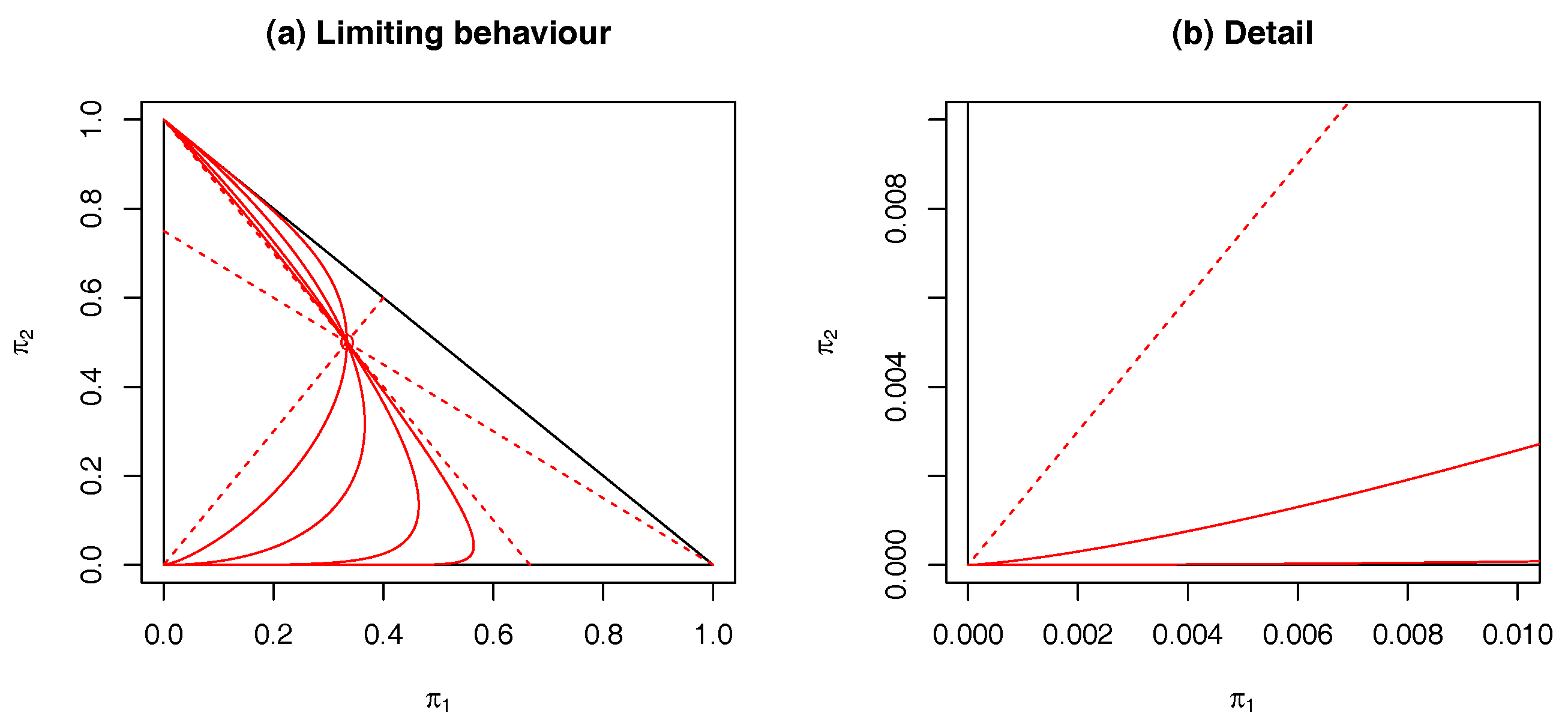
Example 2.
Extended Trinomial Model.
We return to the extended trinomial model in order to visualise and interpret the results of Theorem 1 and its corollaries. In Figure 2a, we select a fixed and a number of different unit vectors, q, to define a set of -exponential families. For each value of q, we compute the corresponding double index. The “generic” case has and . That is, the vector has no ties, and thus has a unique maximum and minimum value. These cases are plotted with a solid line in the figure. We see that these all converge to a vertex, exponentially approaching one of the edges, as predicted. The process of convergence is emphasised in panel (b), showing the convergence in detail.
There are two non-generic cases, where there is a tie for the maximum, or the minimum value. Note that, since the vector is centred and non-zero, all three values cannot be the same. In this case, we have and either or . As the theorem shows, the limit, in any such case, lies on the face spanned by the two largest (smallest) values, with the other limit point being a vertex. The position of the point on the edge is determined by the expression . These geodesics are plotted with a dashed line in the figure. We note that, in this special case, these -geodesics are also -geodesics.
When we look at the set of tangent vectors, we see behaviour considerably at variance with what would be expected in a manifold-based setting. As mentioned above, since we are not working in open sets, care is needed in checking even standard properties of tangent vectors. First, we note that the set of tangent vectors to -geodesic, which meet at a vertex, has a conal, rather than a vector space structure. In addition, if we consider the “generic” case where , then, from Theorem 1 (iv), we have all limiting tangent vectors that are parallel to (a permutation of)
for all such corresponding -geodesics. These are plotted with solid lines in the figure, and a close-up of the local behaviour; panel (b) shows clearly that all tangent vectors have the same limit. Note that this means that the exponential map, which maps tangent vectors to points in a manifold, cannot be uniquely defined at a boundary point. The fact that the set of limiting directions at a vertex is a (closed) cone comes not, principally, from the “generic” case, but, rather, from the case where . In the figure, one such geodesic converging to is shown with a dashed line. However, for this case, the limiting tangent direction depends on , so all values in the relative interior of the cone can be attained, while it is the boundary directions of the cone that come from the generic case.
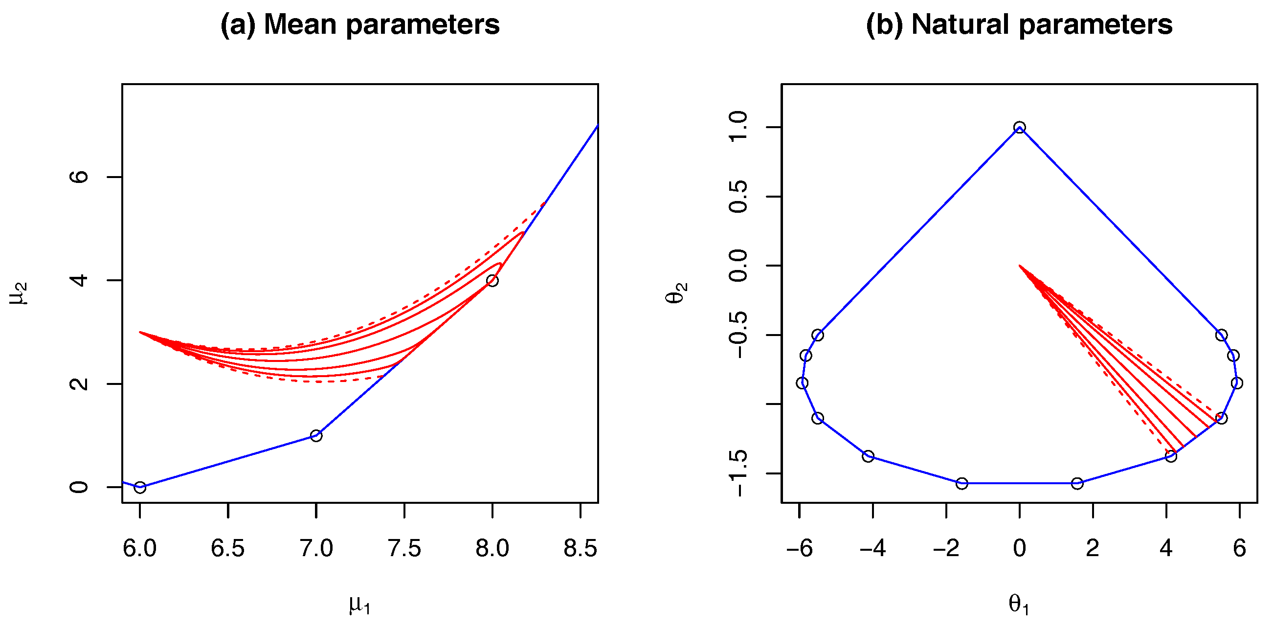
Example 3.
Altham’s Model.
A two-dimensional extension of the binomial family, as described by Altham in [16], is given by
where we take , . This allows both over and under-dispersion relative to the binomial model and for large k can be thought of as a finite, discrete approximation to the normal model (see [15] for more details).
Figure 3 shows, for , some of the details of the boundary convergence of -geodesics that define this family. Panel (a) is shown in the mean, or -affine, parameterisation. The solid lines are “generic” -geodesics that converge to a vertex, as predicted by Theorem 1. As can be seen by close inspection, all of these geodesics have a tangent vector that is parallel to the corresponding edge. The dashed lines correspond to the case where there is a tie in the largest component of the initial direction of the geodesic.
Panel (b) of Figure 3 shows the same geodesics in the natural, or , parameters. Here, the dual polytope is shown as the convex hull of a set of vertices, each of which corresponds to a “direction of recession” (for details, see [12] or [15]). The polar duality can be clearly seen, with all -geodesics cutting an edge in (b) intersecting the corresponding vertex in panel (a), while the dashed lines hit vertices in (b), intersecting edges in (a).
3. Fisher Geodesics
We turn now to the Fisher, or , geodesic in an exponential family embedded in a finite simplex. For completeness, we recall that the 0-representation maps the simplex to the sphere, and the Fisher metric is the pullback of the standard metric on the sphere. Here, we shall define a new class of geometric object—the extended Fisher geodesic—which lies naturally in the extended exponential family.
In an exponential family, Fisher geodesics are the geodesics of the Levi–Civita connection and have the property of being (local) minimisers of path length and energy [17]. They were one of the first differential geometric objects studied in statistics [1]. In general, they cannot be computed in closed form, except in a few special cases, but can be computed numerically using their defining differential equations. Since these equations need to be defined on open sets, the analysis here is required to understand their limiting behaviour in the closure.
In Figure 1b, we see a Fisher geodesic in the extended trinomial model. This is a case where there is a closed form (see [1], p. 32). It can be directly calculated in the -representation of the simplex, given by , . The image of Fisher geodesic connecting and is the set of points of the form
where , and is the positive normalising constant, which ensures . Since we are working in the extended multinomial model, there is no constraint on the positivity of and the figure shows the image of the full great circle in the sphere, which is the Fisher geodesic in the -representation. We can alternatively think of it as the union of Fisher geodesics in the relative interior, which is smoothly connected at the boundary. It is this smooth touching of the boundary that motivated the results in this section. In fact, the curve in Figure 1b was computed by solving the underlying differential equation numerically using the methods of Section 3.2 below. The local solution is guaranteed to exist in open neighbourhoods, but the numerical solution was extended smoothly into, and out of, the boundary. The main result of this section shows, both theoretically and numerically, that this a general property of extended Fisher geodesics in extended exponential families in the simplex.
We note that the way that the -geodesic smoothly intersects with the boundary in Figure 1b is generic in all exponential families, as shown in Theorem 6. However, for clarity, we also note that the closed nature of the -geodesic, seen in the figure, is a special property of multinomial models. This follows since they are equivalent to standard spheres under their Fisher Reimannian structure. Hence, in this special case, the extended geodesics are the images of great circles and hence closed. In general, as illustrated in Example 3, the geodesics do not form closed loops.
3.1. The Fisher Geodesic and the Boundary
In order to define extended Fisher geodesics, we need to consider how to measure the energy of a curve in an extended model. In particular, we need to understand the energy of a path whose limit lies in the boundary, as seen in Figure 1b. The following result on how the Fisher information behaves near the boundary follows from results in [18] and was stated in [15]. It shows the singularity of the metric, in both the mean and natural parameters at the boundary. The importance of this result is to emphasise that standard Riemannian geometry does not extend directly to the boundary of the extended exponential family.
Theorem 2.
(a) Let be a sequence of points in the mean parameter space of an exponential family, lying in , which converge to , which lies on a face of the boundary polytope, defined by the half space, characterised by an equation of the form , for a unit normal vector a.
Let be the Fisher information, its minimum eigenvalue, assumed simple, and a corresponding unit eigenvector, and unique up to overall sign. Then,
and .
(b) Let be the corresponding sequence to in the natural parameters, the Fisher information, with its maximum eigenvalue, assumed simple, a corresponding unit eigenvector, unique up to overall sign. Then,
and , which is the vertex in the polar which corresponds to the face in (a).
From the proof of Corollary 1, we have that the closure, , of an exponential family can be written explicitly as a finite union of exponential families each lying in its own, proper, face. We first define what it means for a curve to be smooth in the closure.
Definition 4.
A -representation of a curve in the closure, , of an exponential family in is
It is defined to be S-smooth in the closure when it can be partitioned into the union of smooth subpaths each in an exponential family,
for , where:
- (i)
- .
- (ii)
- For each ,
- (iii)
- For each , and ,
We denote the set of S-smooth curves as .
A curve in has a finite arc length if
where is the Fisher information in . Furthermore, the curve has finite energy if
It is common, and convenient, in Riemannian geometry [17] (Theorem 13, p. 128), to characterise Levi–Civita geodesics as being local minimisers of the energy functional, since these are the same paths that are local minimisers of the length functional. We follow this approach here when extending the definition of a -geodesic to the extended exponential family.
We can now define an extended geodesic on an extended exponential family.
Definition 5.
Let be an extended exponential family, and let . Define the set of finite energy paths by
Definition 6.
If , we call γ an extended Fisher geodesic if it (locally) minimises the energy functional.
Theorem 3.
(a) Consider a curve , where for and lies in the proper face defined by a support set , i.e., if , then .
Then, the curve has finite energy implies that lies in the tangent space to the proper face defined by the support set .
(b) Let be a p-dimensional exponential family, whose closure is . Let and let lie in a proper face of defined by the index set . If has the property that for and is an extended Fisher geodesic, then we have: in the relative interior, after writing in terms of the mean parameters of as
where are the Christoffel symbols for the Levi–Civita connection of the Fisher metric.
On the boundary, we have that the curve γ has the property that is tangent to the face containing .
Proof.
See Appendix B. ☐
3.2. Computing the Extended Fisher Geodesic
Figure 1b shows an example of a Fisher geodesic’s limiting behaviour. In particular, it is smooth on the boundary. However, it shows more, as we see a smooth curve in the extended multinomial model that has three points lying on the edges and three disconnected, Fisher geodesics in the relative interior. These geodesics are smoothly connected in the extended family. This example motivated our investigation of the properties of extended Fisher geodesics. In this section, we investigate if it is possible to numerically find extended Fisher geodesics for arbitrary exponential families and numerically investigate their limiting properties. We have, from the consideration of the limiting properties of -geodesics, that, near the boundary, the exponential family lies almost parallel to a low-dimensional face of the simplex. Thus, locally -geodesics in general exponential families will behave rather like -geodesics in multinomial families, shown in Figure 1b, and reflect back into the the interior. At least locally, the geodesic behaves like the projection of the continuation of geodesics on the sphere. Example 4 below shows an explicit example of such a solution, where we have added the so-called reflection principle, Definition 7, in order to ensure both uniqueness and numerical stability in the solution.
The characterisation of the exponential family via Equation (1) is the familiar explicit representation in terms of the natural parameters, but is problematic numerically in representing the limiting distributions since the natural parameter needs to be unbounded to attain the boundaries. Thus, we replace this with a -representation, and then, invoking the reflection principle, we will work numerically in a -representation.
From above, a p-dimensional exponential familiy is defined by , an orthonormal set of centred vectors. This set can be extended to form a k-dimensional orthonormal set of centred vectors, by selecting . Within , a -geodesic within this exponential family can be characterised by a set of differential equations of the form: for and ,
where Equation (16) constrains the curve to lie in the space of unit measures, Equation (17) forces the solution to lie in the p-dimensional exponential family, and finally Equation (18) constrains the solution to be a Fisher geodesic inside that family.
In order to solve these equations numerically, we discretise in the standard way, but, near the boundary, we recognise that there is numerical instability in Equations (16)–(18) for small values of . From the analysis of Section 2, we know that the small values are a fundamental part of the limit process. To illustrate such a solution, consider the following example.
Example 4.
Altham’s Model.
We return to Altham’s two-dimensional extension of the binomial family. We take the Equations (16)–(18) and solve them numerically, in order to get an extended Fisher geodesic. This numerical solution is shown in Figure 4, with panel (a) showing the complete extended exponential family and panel (b) showing detail of the boundary behaviour.
As can be seen, in this example, the extended Fisher geodesic smoothly touches the boundary in two places. In fact, we can think of the path as the smooth union of a set of extended geodesics.
As the previous example shows, we can think about the smooth union of extended geodesics. To ensure smoothness, we employ the following idea, which ensures the paths `reflect’ at a boundary and join in a smooth way.
Definition 7.
The reflection principle.
To the conditions of Theorem 3, we add the condition that the limit of the second derivative, , is finite and continuous on the path and use this to smoothly connect extended Fisher geodesics at the boundary.
In Appendix C, we discuss how we implement code that computes smooth unions of extended Fisher geodesics numerically using this principle by working in the parameters.
3.3. Applications
While Fisher geodesics were studied very early in the Information Geometry literature, the importance of their applied utility is still an open question. The geodesic and the corresponding geodesic distance seem to be a natural thing to study and has, for example, found applications in image analysis (see [19,20], for example).
The seminal paper [21] illustrates a very important way that Fisher Riemannian geometry can have an impact on statistical practice. It considers, under regularity, parameter spaces of statistical models as smooth manifolds, and designs highly efficient Markov chain Monte Carlo algorithms by using Langevin methods on Riemannian geometric structures. In our recent paper [18], we showed the way that Fisher geodesics can smoothly attach to the boundaries of exponential families, and how this is one of the ways that the MCMC method achieves its efficiency. The results of this paper give the details of the results announced there.
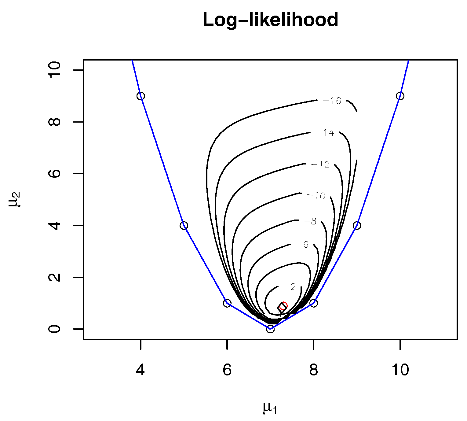
In the paper [18], it was also shown how the boundary effects in extended exponential families mean that the log-likelihood can be very far from approximately quadratic in the mean and natural parameters.
Example 5.
Altham’s model.
Returning to Altham’s model, Figure 5 shows an example of the shape of the log-likelihood function, in the mean parameters, when the maximum likelihood estimate is near the boundary. We see that the log-likelihood is very far from being approximately quadratic.
Example 5 illustrates, in a simple visual way, how the log-likelihood can be far from approximately quadratic when near the boundary. The condition that the maximum likielihood estimate is on, or close to, the boundary is very common in categorical data analysis [9] and other discrete models [11]. This means that that standard iterative gradient based method, such as Newton’s method, can fail in the mean or natural parameters. This was explored in [22] where it was shown that the boundary effects mean that commonly used first order asymptotic analyses, in, say logistic regression, can also fail.
We propose here that the smooth way that the Fisher Riemannian geometry deals with the boundary can be a useful tool to help deal with these problems. If we explore the model space using its Riemannian geodesics structure, we can smoothly reach the boundary. We see that this is in sharp contrast to working in the mean parameters, which, using Newton’s method, would jump outside the boundary, or the natural parameters, which can never reach the boundary in finite time using a gradient approach. We note in fact Amari’s highly efficient natural gradient method [23], while often motivated by divergence ideas, exactly uses the Fisher Riemannian geometry.
Acknowledgments
The authors would like to thank the Engineering and Physical Sciences Research Council (EPSRC) for the support of Grant No. EP/E017878/. We would also like to thank the referees for their very helpful comments.
Author Contributions
Both authors contributed equally to all aspects of this paper.
Conflicts of Interest
The authors declare no conflict of interest.
Appendix A. Proof of Theorem 1
We begin with the following preliminaries. Recall: means that as . It follows that, for :
In particular, for all ,
Again, being continuous at 0 for all ,
Note that we work throughout to first order (only) in .
Differentiating:
In addition, again:
In addition, for a third time:
Using these preliminary results, we can look at limits of the relevant quantities. Throughout defines a reference bin , for which the maximum value is observed.
(i) First look at the bin probabilities.
For j = 0:
For j > 0:
For each and , (A4) gives
(ii) We can now look at the mean parameter for the geodesic
It follows at once from (A15) that:
while, for each ,
Furthermore, using (A3), we have:
while, for each ,
(iii) Next, we look at the Fisher information
(iv) Finally, we look at limiting tangent vectors in (-1)-coordinates.
For :
For :
For :
Appendix B. Proof of Theorem 3
(a) It is convenient to work in the -representation of the simplex i.e., . In , the Fisher metric on all tangent spaces is induced by the identity matrix in and this agrees with the Fisher metric for all tangent spaces of .
We write
The image of in the is
and its tangent vector is
Thus, for , the squared length of the tangent vector is
For any index i such that , suppose . There are two cases. First, for , so that
which is unbounded above as . The second case, , can not happen due to the non-negativity of probabilities. Thus, we have
Appendix C. Numerically Solving for Extended Fisher Geodesic
To numerically solve Equations (16)–(18), we have found that it is convenient to work in the -representation of the simplex, that is, . In these parameters, the defining equations, in the relative interior, are
We use the package deSolve in R [24], to numerically solve the Equations (A29)–(A31). This method discretises the equations and solves them iteratively. At iteration s, we have state variables and . From the standard theory of ODE, in the relative interior, such state variables are enough to determine what happens at the next state by solving the linear equations, which are the discrete version of Equations (A29)–(A31).
At the boundary, where at least one , the corresponding linear equations are singular and do not define a unique next state. We therefore apply the reflection principle to extend the path through this singularity. To apply the principle numerically, we add to the algorithm the condition that whenever the value of
we reflect in this boundary by changing this component of the tangent vector to . This means that the path in -space is locally of the form
in a neighbourhood of . In terms of the -parameters, this gives
which means at , where the path touches the boundary, we have that the tangent is zero, as required by Theorem 3(b) but also that the second derivative is finite and continuous as required by the reflection principle.
(b) We use the characterisation of a Fisher geodesic as being a local minimiser of the energy functional among smooth curves. We follow the standard argument using the calculus of variations, which give the geodesic Equations (15) within the relative interior. A path that is smooth in the extended exponential family will have finite energy if the tangent vector is parallel to the boundary. Since the geodesic is a local minimiser, it must have finite energy. This gives the final boundary condition.
References
- Amari, S.-I. Differential-geometrical methods in statistics. In Lecture Notes in Statistics; Springer: New York, NY, USA, 1985; Volume 28. [Google Scholar]
- Amari, S.-I.; Barndorff-Nielsen, O.E.; Kass, R.E.; Lauritzen, S.L.; Rao, C.R. Differential Geometry in Statistical Inference; IMS Lecture Notes-Monograph Series; IMS: Hayward, CA, USA, 1987. [Google Scholar]
- Barndorff-Nielsen, O.E. Information and Exponential Families in Statistical Theory; John Wiley & Sons, Ltd.: Chichester, UK, 1978. [Google Scholar]
- Kass, R.E.; Vos, P.W. Geometrical Foundations of Asymptotic Inference; John Wiley & Sons, Inc.: Hoboken, NJ, USA, 1997. [Google Scholar]
- Amari, S.-I. Information Geometry and Its Applications; Springer: Tokyo, Japan, 2016. [Google Scholar]
- Brown, L.D. Fundamentals of Statistical Exponential Families with Applications in Statistical Decision Theory; Lecture Notes-Monograph Series; IMS: Hayward, CA, USA, 1986; Volume 9. [Google Scholar]
- Critchley, F.; Marriott, P. Information Geometry and Its Applications: An Overview; Computational Information Geometry; Springer: Cham, Switzerland, 2017; pp. 1–31. [Google Scholar]
- Agresti, A. Categorical Data Analysis, 3rd ed.; Wiley: Hoboken, NJ, USA, 2013. [Google Scholar]
- Geyer, C.J. Likelihood inference in exponential families and directions of recession. Electron. J. Stat. 2009, 3, 259–289. [Google Scholar] [CrossRef]
- Lauritzen, S.L. Graphical Models; Clarendon Press: Oxford, UK, 1996. [Google Scholar]
- Rinaldo, A.; Feinberg, S.; Zhou, Y. On the geometry of discrete exponential families with applications to exponential random graph models. Electron. J. Stat. 2009, 3, 446–484. [Google Scholar] [CrossRef]
- Fienberg, S.E.; Rinaldo, A. Maximum likelihood estimation in log-linear models. Ann. Stat. 2012, 40, 996–1023. [Google Scholar] [CrossRef]
- Rauh, J.; Kahle, T.; Ay, N. Support sets in exponential families and oriented matroid theory. Int. J. Approx. Reason. 2011, 52, 613–626. [Google Scholar] [CrossRef]
- Geiger, D.; Meek, C.; Sturmfels, B. On the toric algebra of graphical models. Ann. Stat. 2006, 34, 1463–1492. [Google Scholar] [CrossRef]
- Critchley, F.; Marriott, P. Computing with Fisher geodesics and extended exponential families. Stat. Comput. 2016, 26, 325–332. [Google Scholar] [CrossRef]
- Altham, P. Two generalizations of the binomial distribution. Appl. Stat. 1978, 27, 162–167. [Google Scholar] [CrossRef]
- Petersen, P. Riemannian Geometry, 2nd ed.; Graduate Texts in Mathematics; Springer: New York, NY, USA, 2006; Volume 171. [Google Scholar]
- Critchley, F.; Marriott, P. Computational Information Geometry in Statistics: Theory and practice. Entropy 2014, 16, 2454–2471. [Google Scholar] [CrossRef]
- Mio, W.; Badlyans, D.; Liu, X. A computational approach to Fisher information geometry with applications to image analysis. In Energy Minimization Methods in Computer Vision and Pattern Recognition; Springer: Berlin, Germany, 2005. [Google Scholar]
- Peter, A.; Rangarajan, A. Shape analysis using the Fisher-Rao Riemannian metric: Unifying shape representation and deformation. In Proceedings of the 3rd IEEE International Symposium on Biomedical Imaging: Nano to Macro, Arlington, VA, USA, 6–9 April 2006. [Google Scholar]
- Girolami, M.; Calderhead, B. Riemann manifold Langevin and Hamiltonian Monte Carlo methods. J. R. Stat. Soc. B 2011, 73, 123–214. [Google Scholar] [CrossRef]
- Anaya-Izquierdo, K.; Critchley, F.; Marriott, P. When are first-order asymptotics adequate? A diagnostic. STAT 2014, 3, 17–22. [Google Scholar] [CrossRef]
- Amari, S.I. Natural gradient works efficiently in learning. Neural Comput. 1998, 10, 251–276. [Google Scholar] [CrossRef]
- R Core Team. R: A Language and Environment for Statistical Computing; R Foundation for Statistical Computing: Vienna, Austria, 2016. [Google Scholar]
Figure 1.
Key geodesics in the extended trinomial model.
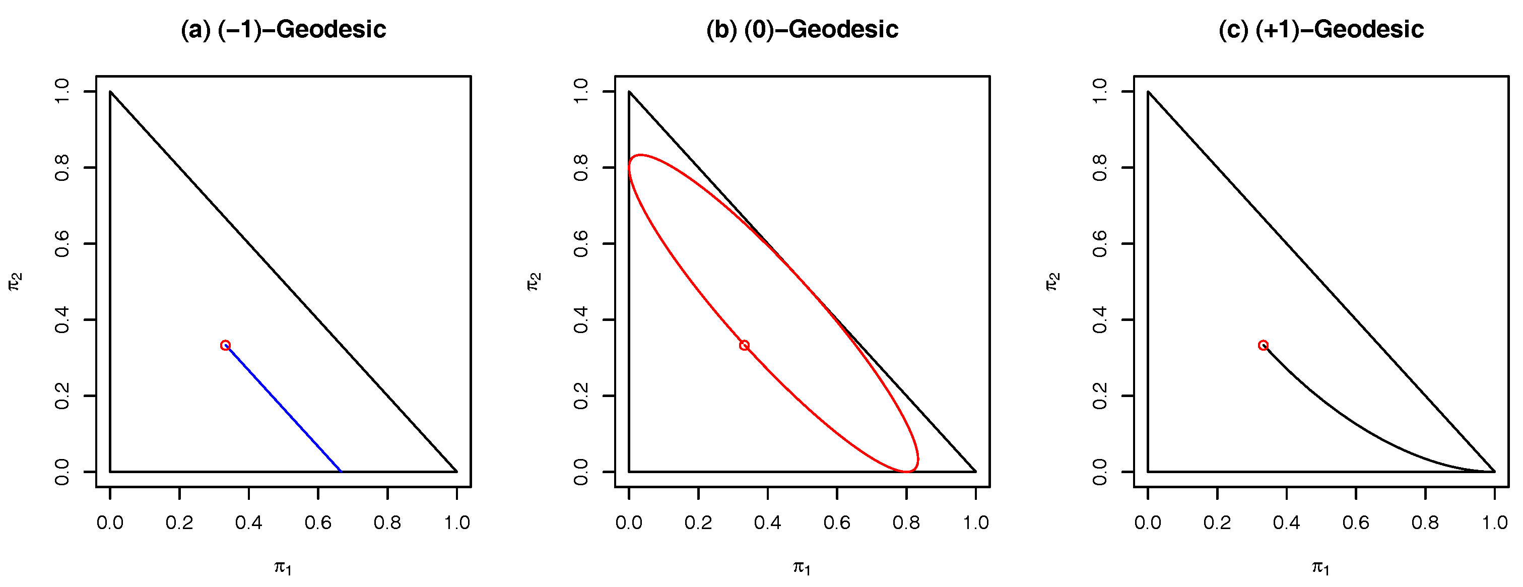
Figure 2.
A set of -geodesics in the extended trinomial model.

Figure 3.
A set of -geodesics in Altham’s model.

Figure 4.
Extended Fisher geodesic in Altham’s model.
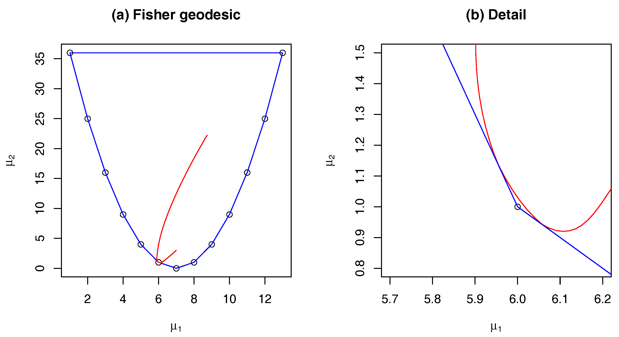
Figure 5.
Contours of the log-likelihood in Altham’s model.

© 2017 by the authors. Licensee MDPI, Basel, Switzerland. This article is an open access article distributed under the terms and conditions of the Creative Commons Attribution (CC BY) license (http://creativecommons.org/licenses/by/4.0/).
Share and Cite
MDPI and ACS Style
Critchley, F.; Marriott, P. On the Limiting Behaviour of the Fundamental Geodesics of Information Geometry. Entropy 2017, 19, 524. https://doi.org/10.3390/e19100524
AMA Style
Critchley F, Marriott P. On the Limiting Behaviour of the Fundamental Geodesics of Information Geometry. Entropy. 2017; 19(10):524. https://doi.org/10.3390/e19100524
Chicago/Turabian StyleCritchley, Frank, and Paul Marriott. 2017. "On the Limiting Behaviour of the Fundamental Geodesics of Information Geometry" Entropy 19, no. 10: 524. https://doi.org/10.3390/e19100524
Note that from the first issue of 2016, this journal uses article numbers instead of page numbers. See further details here.