Abstract
This paper considers a two-way relay network, where two legitimate users exchange messages through several cooperative relays in the presence of an eavesdropper, and the Channel State Information (CSI) of the eavesdropper is imperfectly known. The Amplify-and-Forward (AF) relay protocol is used. We design the relay beamforming weights to minimize the total relay transmit power, while requiring the Signal-to-Noise-Ratio (SNRs) of the legitimate users to be higher than the given thresholds and the achievable rate of the eavesdropper to be upper-bounded. Due to the imperfect CSI, a robust optimization problem is summarized. A novel iterative algorithm is proposed, where the line search technique is applied, and the feasibility is preserved during iterations. In each iteration, two Quadratically-Constrained Quadratic Programming (QCQP) subproblems and a one-dimensional subproblem are optimally solved. The optimality property of the robust optimization problem is analyzed. Simulation results show that the proposed algorithm performs very close to the non-robust model with perfect CSI, in terms of the obtained relay transmit power; it achieves higher secrecy rate compared to the existing work. Numerically, the proposed algorithm converges very quickly, and more than 85% of the problems are solved optimally.
1. Introduction
Due to the openness and the broadcast property of wireless communication, network security becomes a challenging issue. The physical layer security technique becomes appealing, because it guarantees the information being only accessed by the legitimate users rather than eavesdroppers. It makes use of the physical characteristics of wireless channels and is free of a security key, so that the information is transmitted securely in the sense that it can be decoded by legitimate users, but not eavesdroppers.
Physical layer security is widely studied from both the information theory aspect and the signal processing aspect for wiretap channels, like broadcast wiretap channels and Multiple-Input-Multiple-Output (MIMO) wiretap channels. The secure communication is managed through multiple-antenna system [1,2,3,4,5,6,7,8,9] or node cooperation [10,11]. Research works on node cooperation are well explored. It is suitable for low-complexity networks, which cannot afford multiple antennas. Cooperative relay networks with Amplify-and-Forward (AF) [12,13,14,15] or Decode-and-Forward (DF) [16,17] protocols are mostly investigated. For one-way relay networks, the authors in [18,19] design the relay beamforming weights to maximize the secrecy rate and to minimize the relay transmit power; the secrecy outage probability is analyzed for both half-duplex [20] and full-duplex relay networks [21]; in [22], the optimal relay selection schemes are considered, for both AF and DF protocols; the secure energy efficiency maximization model is proposed in [23]; the asymptotic secrecy performance for the large-scale MIMO relaying scenario is analyzed in [24], which concludes that the AF protocol is a better choice compared to DF under large transmit powers. Compared to one-way relay, two-way relay networks are more efficient for communications between user pairs. In [25], the minimum per-user secrecy rate is maximized, and the source power allocation is analyzed, where the relay beamforming vector lies in the nullspace of the equivalent channel of the relay link from user nodes to the eavesdropper.
All the aforementioned references suppose that the CSI from users and from relays to eavesdroppers are perfectly known. In fact, it is very difficult to obtain the perfect CSI of the eavesdroppers. Assuming that no CSI of eavesdroppers is known, artificial noise is introduced in the literature, and enhances security: Wang et al. proposes a cooperative artificial noise transmission-based secrecy strategy and summarizes the relay beamforming design and power allocation problems as second order cone programming and linear programming problems [14], respectively; Salem et al. sends the artificial noise in the nullspace of the legitimate channel and compares the cases in which that all relays are working and that only the best relay is used [15]. In [26], no CSI of eavesdroppers and imperfect CSI between users and jammers are assumed, and the secrecy performance is analyzed for the Cooperative Jamming (CJ) technique. Networks with imperfect CSI are often considered, as well. The multi-user downlink channel is considered in [27], where the lower bound of the sum secrecy rate is maximized, and semi-definite relaxation and first order Tailor extension techniques are applied. In [28], a multiple-antenna AF relay network with partial CSI and a bounded error region is considered, which maximizes the worst case secrecy rate, where a rank two relay beamformer is constructed via singular value decomposition. The secure communication switches between the DF relay protocol and the CJ technique in [29], and the authors provide robust designs for the secrecy rate maximization and secrecy outage probability minimization problems. In [30], both the source and the relay have multiple antennas, where they jointly design source and relay beamforming matrices, to minimize the relay power with Quality of Service (QoS) constraints. The worst case SNR at the eavesdropper is considered, which is approximated by its upper bound. For a two-way relay network with two users and one eavesdropper, Wang et al. assumes no CSI of the eavesdropper is available [31]. The artificial noise technique is applied, and the relay transmit power for signals is minimized, while the QoS of two users are guaranteed. A second order cone programming problem is formed and solved by the interior point method.
In this paper, we consider the same communication model as [31]. Differently, we assume that there is imperfect CSI from users and relays to the eavesdropper. By designing the relay beamforming weights, we build up the model to minimize the relay transmit power, while the QoS of the legitimate users are guaranteed, and the worst case achievable rate of the eavesdropper is upper bounded. Compared to [31], the proposed model makes use of the imperfect CSI, and guarantees that the achievable rate of the eavesdropper is very low. Compared to the optimization model in [31], the proposed model has an extra robust constraint for the eavesdropper, which leads to a much more difficult robust optimization problem [32]. Usually, such problem is NP-hard. There is a lack of an efficient method to solve this kind of problem. We propose an efficient iterative algorithm to solve the problem with the line search technique. In each iteration, two Quadratically-Constrained Quadratic Programming (QCQP) subproblems and a one-dimensional subproblem are solved optimally; the iterative points always remain feasible. The optimality conditions of the robust optimization problem are also analyzed. Simulation results show that compared to [31], our algorithm achieves a higher secrecy rate; the proposed algorithm is efficient and converges very quickly; numerically, more than 85% of the problems are solved optimally. The main contributions of our paper are listed as follows:
- A new model to design the relay beamforming weights is proposed with the assumption of imperfect CSI and summarized as a robust optimization problem.
- A novel algorithm is proposed, where the line search technique is applied. A sequence of QCQP subproblems and one-dimensional subproblems is solved optimally. The feasibility is preserved during iterations. Simulation results verify the efficiency of the proposed algorithm.
- The optimality properties of the robust optimization problem are analyzed. Numerically, most problems are solved optimally.
The rest of the paper is organized as follows. The system model of the two-way relay network with one eavesdropper is shown in Section 2. In Section 3, the corresponding optimization problem is summarized, and a novel algorithm is proposed. Simulation results are shown in Section 4. The conclusion is summarized in Section 5.
Notations: Uppercase and lowercase bold-faced letters denote matrices and column vectors, respectively. and represent the real and complex domain, respectively. , and represent the Hermitian, transpose and conjugate of a matrix, respectively. represents the absolute value. By default, is the two-norm of a vector. is the Frobenius norm of a matrix. is the mathematical expectation of a random variable. represents the trace of a matrix. means the real part of a scaler, a vector or a matrix. represents the largest eigenvalue of a Hermitian matrix. is the diagonal matrix with diagonal entries as the elements of vector ; is the diagonal matrix with the same diagonal entries as matrix . represents that the random variable x obeys a Gaussian distribution with the mean as and variance as .
2. System Model
We consider a half-duplex wireless communication system where two legitimate users Alice () and Bob () exchange messages with N relay nodes , in the presence of an eavesdropper Eve, who eavesdrops signals from the two users and relays passively, as illustrated in Figure 1. Suppose each user, each relay and Eve have a single antenna. The AF relay protocol is applied.
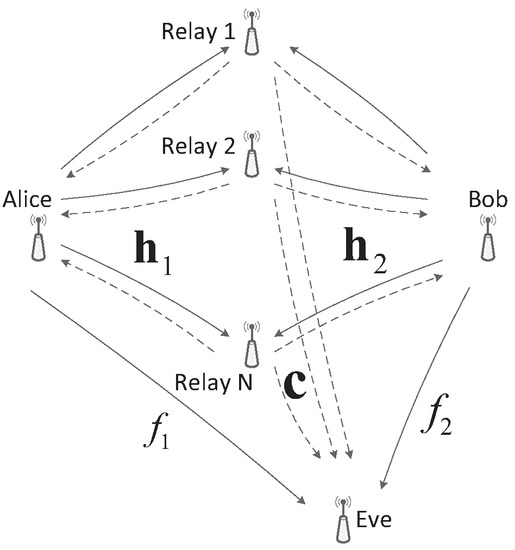
Figure 1.
Secure communication model for the two-way relay network.
We assume that the perfect CSI between two users and relays is known, as , . However, due to limited feedback, it is difficult to obtain perfect CSI of Eve. Thus we assume the imperfect CSI for the channels from users and relays to the eavesdropper, and the norm-bounded error channel estimation is considered. The CSI between the users and the eavesdropper, , and that between relays and the eavesdropper, , are assumed to be imperfect and are estimated with bounded errors:
Here, and are the estimations, which are achievable; and are the bounded errors, . Such assumptions are practical in scenarios where some users and relays are turned into eavesdroppers and their CSI have already been partially estimated.
In the first phase, Alice and Bob transmit , to all relays, respectively, where is the fixed transmit power and is the information symbol with . Then, relays receive:
where is the noise at relays with zero mean and covariance matrix as .
In the second phase, the n-th relay multiples its received signal by its beamforming weight and then broadcasts the signal to both users. Thus, the vector transmitted by relays is represented as , where and . Alice receives:
where is the local noise. It consists of the self-canceled signal, which is perfectly known by Alice and is canceled locally, the desired signal from Bob and the noise. The received signal at Bob has a similar expression.
Since the two source nodes subtract their self-canceled terms, the SNRs achieved at Alice and Bob can be respectively expressed as:
where , .
In both phases, Eve listens to the users and relays and receives signals as:
where and are the noise at Eve in the two phases, respectively. Suppose Eve is intelligent and tries to decode signals by combining the information received in both phases, which is expressed as:
where:
Suppose all the transmit signals and all the noises are independent of each other. The achievable rate of Eve is denoted as:
Here, , and:
The detailed deduction is shown in Appendix A. The definitions of and , are shown in (5) and (1).
We want to design the relay beamforming vector , to minimize the total relay transmit power, while requiring the SNRs of two legitimate users to be guaranteed and the achievable rate of Eve to be upper-bounded. Due to the imperfect CSI of Eve, the worst case achievable rate is considered. The model is summarized as follows:
where the relay transmit power is:
and , , are the given thresholds. Here the achievable rate of Eve is required to be below the given threshold under any variation of channel coefficients. Due to the constraint (7c), we can guarantee that the achievable rate of Eve is very low. Because of this constraint, problem (7) is a robust optimization problem. It is equivalent to a QCQP problem with infinite constraints, which is usually NP-hard. In the following section, the problem is solved by a novel algorithm.
Remark 1.
The model with perfect CSI and that with no CSI [31] are two extreme cases of the model (7). If we let , then the model degenerates to that with perfect CSI; if the parameters ε and , and go to infinity, then it becomes the model with no CSI.
3. Robust Optimization Model
In this section, we first approximate Problem (7) by a new robust optimization problem, where there are less parameters with uncertainty. Then, we propose a novel efficient algorithm to solve the approximated problem.
3.1. Robust Model Formulation
In Problem (7), there are several parameters with uncertainty, which are coupled together and thus make the problem intractable. We tighten the constraint (7c) by replacing with its upper bound , where ,
It holds that:
for any . The detailed deduction is shown in Appendix B. Problem (7) is tightened as the following robust optimization problem:
Here, , and in Constraint (9c), is the equivalent form as . The parameters , in Problem (7) have been eliminated. Accordingly, any feasible point of Problem (9) is a feasible point of Problem (7).
In the rest of this section, we focus on solving the tightened Problem (9).
3.2. Algorithm Preserving Feasibility
As a robust optimization problem, Problem (9) is still difficult to solve and generally NP-hard. Usually, robust optimization problems are approximated, and the parameters with uncertainty are eliminated. Then, the classical optimization technique is used, and the approximated problem is solved directly. However, sometimes, the approximated problem is not a “good” approximation. It may cut off parts of the feasible region of the original problem and consequently lose the optimality property or even feasibility. To avoid these disadvantages, we propose an efficient iterative algorithm to solve Problem (9). In each iteration, the iterative point is updated by the line search technique, and it is always a feasible point of Problem (9). The optimality properties of Problem (9) are analyzed, as well.
3.2.1. Initialization
First, we initialize the algorithm by solving the following subproblem:
Here, . , , and ; is a scalar, and is a positive integer. and are two parameters to keep the initial point as an interior point of Problem (9).
By transformation, Equation (10) is equivalent to the following QCQP subproblem.
where , , , , , and are defined below (3), . Since Subproblem (11) only has three constraints, it is solved optimally by the Semi-Definite Relaxation (SDR) method [33,34].
Here, the constraints in Problem (9) are tightened as (10b) and (10c). The following lemma shows that solving (10) provides an initial feasible point of Problem (9).
Lemma 1.
The optimal solution of subproblem (10), , is an interior point of problem (9).
The proof is shown in Appendix C. is a strictly feasible rather than a feasible point of Problem (9), thanks to the control parameters and in Subproblem (10).
3.2.2. Iterations Applying the Line Search Technique
In the k-th iteration, suppose the iterative point is an interior point of Problem (9) satisfying:
We will update using the line search technique [35] and preserve its feasibility according to Problem (9).
First, we solve two QCQP subproblems to obtain the search direction. The following subproblem is formulated:
It is equivalent to the subproblem below:
where . Let , and it is further transformed into the following QCQP subproblem:
Here:
It is solved optimally by the SDR method. Let be the optimal solution of (13). Then, , as satisfies (12b).
Taking into Problem (9) and introducing the parameters and , we obtain the subproblem below:
It is equivalent to the QCQP subproblem with three constraints:
where and . , , and , are defined below (11). It is solved optimally by the SDR method. Let be the optimal solution of Subproblem (15). Apparently satisfies (12a), but it may not satisfy (12b). Thus, we search along the line to find a new iterative point , which satisfies (12).
Next, we solve a one-dimensional subproblem to obtain the stepsize. Denote t as the stepsize. We calculate the stepsize t, so that the new iterative point satisfies (12) and improves the objective function value of (9). The corresponding subproblem to obtain the stepsize is as follows:
For simplicity, we let and represent and , respectively. Denote , for . Then, the parameters are defined as:
Theorem 1.
For any t satisfying Constraints (16b) and (16c), satisfies (12). Let be the optimal stepsize obtained from Subproblem (16), then the iterative point is updated as . By such an update strategy, is a feasible point of Problem (9), and the objective function of (9) decreases monotonically in each iteration.
The detailed proof is shown in Appendix D. As a one-dimensional QCQP problem, Subproblem (16) is solved optimally by the analysis of line segment intersections, which is omitted due to the limited space. We might encounter the situation that , where the iterative point gets stuck at some point. In this case, we increase the parameter in Subproblem (16), hoping that the iterations continue, and the objective function is further improved.
3.2.3. Algorithm Framework and Optimality Analysis
The complete algorithm framework is described in Algorithm 1 on the next page.
| Algorithm 1: Robust optimization algorithm |
 |
In Algorithm 1, since the iterative points are all feasible for Problem (9) and the objective function decreases monotonically, the objective function value converges eventually. The obtained solution of Algorithm 1 is at least a feasible point of Problem (9) and, thus, is a feasible point of Problem (7). The following theorem shows the optimality property of Problem (9), whose proof is given in Appendix E.
Theorem 2.
If δ goes to infinity and , then is the optimal solution of Problem (9).
Further numerical analysis for the optimality property is shown in Section 4.
4. Simulations
In this section, the performance of the proposed algorithm is evaluated. Each element of the channel coefficients between each user and relays , is randomly generated according to the complex Gaussian distribution . The channel coefficients from users to Eve , , obey . The channel coefficient from each relay to Eve is randomly generated according to , where different values of represent different distances between relays and Eve. The CSI estimated error bound from relays to Eve is , and that from each user to Eve is , . Let all the local noise covariance be the same: . Let the SNR thresholds for both legitimate users be the same: , . In the proposed algorithm, the stopping parameter and the initial value of the parameter are set as and one, respectively; if there is no specific explanation, the stopping parameter and the parameter are set as 15 and , respectively. In the proposed algorithm, parameters and are used to keep the iterative points as the interior points of Problem (9). For each plotted point, 1000 realizations are generated, and the average result is shown. Each QCQP subproblem with dimension higher than one is solved by the SDR method, which is implemented based on the software CVX (Version 2.0) [36].
First we compare our proposed algorithm and the non-robust model with perfect CSI. The non-robust model is problem (7) with given , , for , which is a QCQP problem and solved optimally by the SDR method. In Figure 2, the relay transmit power obtained by both algorithms are depicted, with respect to different relay numbers and different SNR thresholds . It indicates that the performance of the proposed algorithm is very close to the non-robust model, which verifies the efficiency of the proposed algorithm. Our proposed model works better to balance the performance and the feedback overhead, because the perfect CSI requires more feedback. It is observed that relays use less total power when more relays are involved in the transmission process. This illustrates the effectiveness of node cooperation. Also, more relay transmit power is used when increases.

Figure 2.
Comparison between the proposed algorithm and the non-robust model with perfect CSI, with respect to different relay numbers and different . The same colored circle and star marks represent for the proposed algorithm and the non-robust model, respectively. Here, and .
Second, we compare our proposed algorithm with the model in [31] (Section V), where both algorithms are designed for the same communication model. In [31], no CSI of Eve is assumed, and the artificial noise technique is applied. Assuming that the total relay power is fixed, the model in [31] is to minimize the relay transmit power for signals and let relays use the rest of the power to send the artificial noise. The corresponding optimization problem is just Problem (7) without Constraint (7c):
Let and be the relay power for signals obtained by our proposed algorithm solving (7) and by the method in [31] solving (17), respectively. Apparently, . In the comparison, for fairness, we suppose that both algorithms use the same total relay transmit power : the proposed algorithm uses all the power to transmit signals; Wang et al. uses power to transmit signals and power to transmit the artificial noise [31]. This is illustrated in Table 1.

Table 1.
Illustration of relay power allocation of Algorithm 1 and [31].
In this case, the achievable rate of Eve by [31] is calculated as:
where and is defined below (6). Based on the above assumptions, we plot the achieved secrecy rate by the two algorithms with respect to different relay numbers and different in Figure 3. The parameter is the upper bound of the achievable rate of Eve in Algorithm 1. It does not appear in the model of [31], but affects its achieved secrecy rate through . We observe that the achieved secrecy rate by the proposed algorithm is higher than that of [31], and the difference becomes larger with the increment of relay numbers. This shows the beneficial effect of using CSI.

Figure 3.
Comparison between Algorithm 1 and [31] which has no CSI, with respect to different relay numbers and different . Here, and .
Third, we test the sensitivity of the proposed algorithm according to parameters and . The two parameters are used to keep the iterative points as the interior point of Problem (9) and control the accuracy of the achieved solution. Figure 4 shows the results by the proposed algorithm with three groups of parameters: = 0.1, = 15; = 0.1, = 20; = 0.01, = 15. The three curves representing the three groups are close to each other, which implies that the algorithm is not sensitive to the parameters.
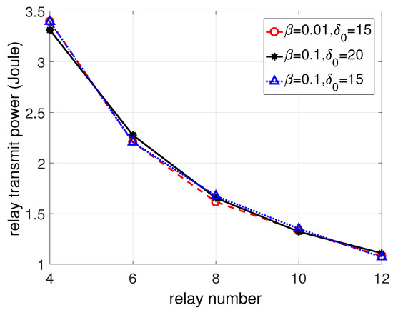
Figure 4.
Achieved relay transmit power by the proposed algorithm with different parameters. Here, , , .
Fourth, the achieved relay transmit power with respect to the iterations is plotted in Figure 5. From top to bottom are the curves representing the relay number N = 4, 8 and 12. The three convergence curves show similar trends, regardless of N. Figure 5 shows that the objective function reduces rapidly in the first three iterations and converges in about five iterations. The observation coincides with the conclusion in Theorem 1 that the objective function value decreases monotonically. It also provides numerical evidence that our proposed algorithm converges very quickly.

Figure 5.
Convergence curves for . Here, , and .
Fifth, we analyze the optimality of the achieved solutions by our proposed algorithm. In the algorithm framework, there are two stopping criteria. The first criterion is that , and and are sufficiently close to each other. According to Theorem 2, the iterative point satisfying this criterion is roughly the optimal solution of Problem (9). The second stopping criterion is simply that . It only guarantees feasibility rather than optimality. In Table 2, we list the number of realizations out of the 1000 that exit the algorithm by satisfying the first stopping criterion, with respect to different relay numbers. It indicates that more than 85% of the realizations obtain the optimal solution of Problem (9). This shows that our proposed algorithm is efficient to solve the problem.
Table 2.
Number of realizations out of 1000 to exit Algorithm 1 by satisfying the first stopping criterion, with , and .
From the above simulation results, we can see that our proposed algorithm is efficient and converges very quickly.
5. Conclusions
In this paper, we consider the two-way relay wiretap channel, with two users, N relays and one eavesdropper. The CSI from users and from relays to Eve is estimated with bounded error. We design the relay beamforming weights to minimize the total relay transmit power, while requiring the users’ SNRs to be higher than the given thresholds and guaranteeing Eve’s worst case rate to be upper bounded. For the robust optimization problem, we propose an algorithm to solve it iteratively and preserve feasibility during iterations. In each iteration, the line search technique is applied. We update the search direction and the stepsize by optimally solving two QCQP subproblems and a one-dimensional subproblem, respectively. The optimality property of the robust optimization problem is analyzed, as well. Simulations show that our proposed algorithm obtains very close relay transmit power to the non-robust model; compared to [31], the proposed algorithm achieves higher secrecy rate. Numerically, the proposed algorithm converges very quickly, and more than 85% of the problems are solved optimally.
Acknowledgments
This work is partly supported by the the National Natural Science Foundation of China (NSFC) 11771056, 11471052, 11401039, 91630202 and 11331012.
Author Contributions
Wenbao Ai and Cong Sun conceived of and designed the model and the algorithm. Ke Liu and Dahu Zheng performed the experiments. Cong Sun and Ke Liu analyzed the data. Cong Sun wrote the paper. All authors have read and approved the final manuscript.
Conflicts of Interest
The authors declare no conflict of interest. The founding sponsors had no role in the design of the study; in the collection, analysis or interpretation of data; in the writing of the manuscript; nor in the decision to publish the results.
Appendix A. Deduction of (6)
The last equality holds due to the following lemma:
Lemma A1.
The following equality holds for any and , :
It is trivial to prove this lemma by expanding the left term.
Appendix B. Deduction of (8)
First, we show a lemma that will be used next.
Lemma A2.
Suppose and are two n-dimensional complex vectors. Then, holds for any . The equality holds if and only if .
Proof.
Let and be the real and imaginary part of , respectively, and define and similarly.
Then:
Thus, . The necessary condition to maximize is that and are parallel to and , respectively. This means that should be parallel to . Further with the condition , we can deduce the conclusion. ☐
From Lemma A2, we deduce that:
holds for all , , and that:
Then, we have:
which holds for any , .
Appendix C. Proof of Lemma 1
We prove the conclusion by showing that any feasible point of Subproblem (10) is a strictly feasible point of Problem (9). Suppose is a feasible point of Subproblem (10), which satisfies Constraints (10b) and (10c).
1. It holds that:
for . Thus, strictly satisfies Constraint (9b).
2. First, we prove that holds for all . Given that and , it holds that:
for all . Here, ; the first inequality applies the norm inequality and the property of the Rayleigh quotient; the second inequality comes from that:
with and defined below (10).
As satisfies Constraints (10c), it holds that:
for all . (A2) is an equivalent form as . Thus, strictly satisfies Constraint (9c).
Summarizing the two points, we obtain the conclusion that any feasible point of Subproblem (10) is a strictly feasible point of Problem (9). Consequently, Lemma 1 holds. ☐
Appendix D. Proof of Theorem 1
Our proof is divided into two parts. The first part is to prove that satisfies (12), for any stepsize satisfying (16b) and (16c); is an interior point of Problem (9). Suppose t is any stepsize satisfying (16b) and (16c). Due to Constraint (16b), satisfies Constraint (12a).
Next, we prove that satisfies Constraint (12b). Let:
where and are defined below (16), , and .
1. For all , we deduce that:
Here, and are defined below (16). The inequality applies Lemma A2 and the property of the Rayleigh quotient.
2. Similarly, we deduce that:
for all .
3. For simplicity, denote . Then, we have:
Then, we deduce that:
Thus, , for all .
Due to Constraint (16c), we have that . Besides, combining 1–3, we can deduce that:
That is, , for all . Through equivalent reformulation, we deduce that satisfies Constraint (12b). Thus, it satisfies (12), and it is an interior point of Problem (9). Let t be , then is an interior point of Problem (9).
In the second part, we prove that the objective function of Problem (9) decreases monotonically in each iteration. First, we prove that is always feasible for Subproblem (16) in any iteration. Let k be the iteration index. In the initial iteration (), corresponds to , which is the optimal solution of the initial Subproblem (10). As satisfies (10b), we have that satisfies Constraint (16b). Since satisfies (10c), we deduce that:
Here, . The deduction is similar to (A1). Then, we have , that is satisfies (16c). Thus, is feasible for Subproblem (16) in the initial iteration .
When , represents , which was updated in the -th iteration: . In this case, it is trivial to show that satisfies Constraints (16b) and (16c). The detailed proof is omitted.
Thus, is always feasible for Subproblem (16) in any iteration. Since is the optimal solution of (16), it holds that , that is . This means the objective function of Problem (9) decreases monotonically in each iteration. ☐
Appendix E. Proof of Theorem uid26
For , as any feasible point of Problem (9), there exists a vector , such that holds for all . We define such and as “a robust pair”.
Obviously, in Algorithm 1, and consist of a robust pair, for any k. If goes to infinity and , then goes to zero, and is the optimal solution of the following subproblem:
Next, we shall prove the conclusion by contradiction. Suppose is not the optimal solution of Problem (9), then there must exist another feasible point of (9), , and . Let and be a robust pair. Then, the following inequalities hold:
This shows that is a feasible point of Subproblem (A3). Further the relation shows that has a lower objective function value of (A3) compared to .
This contradicts the fact that is the optimal solution of (A3). Thus, the assumption is incorrect. must be the optimal solution of Problem (9). ☐
References
- Oggier, F.; Hassibi, B. The Secrecy Capacity of the MIMOWiretap Channel. IEEE Trans. Inf. Theor. 2011, 57, 4961–4972. [Google Scholar] [CrossRef]
- Lin, P.H.; Lai, S.H.; Lin, S.C.; Su, H.J. On Secrecy Rate of the Generalized Artificial-Noise Assisted Secure Beamforming for Wiretap Channels. IEEE J. Sel. Areas Commun. 2013, 31, 1728–1740. [Google Scholar] [CrossRef]
- Wang, H.M.; Zheng, T.; Xia, X.G. Secure MISO Wiretap Channels with Multiantenna Passive Eavesdropper: Artificial Noise vs. Artificial Fast Fading. IEEE Trans. Wirel. Commun. 2015, 14, 94–106. [Google Scholar] [CrossRef]
- Chen, X.; Zhang, Y. Mode Selection in MU-MIMO Downlink Networks: A Physical-Layer Security Perspective. IEEE Syst. J. 2015, 11, 1128–1136. [Google Scholar] [CrossRef]
- Kapetanovic, D.; Zheng, G.; Rusek, F. Physical layer security for massive MIMO: An overview on passive eavesdropping and active attacks. IEEE Commun. Mag. 2015, 53, 21–27. [Google Scholar] [CrossRef]
- Cumanan, K.; Ding, Z.; Sharif, B.; Tian, G.Y.; Leung, K.K. Secrecy Rate Optimizations for a MIMO Secrecy Channel with a Multiple-Antenna Eavesdropper. IEEE Trans. Veh. Technol. 2014, 63, 1678–1690. [Google Scholar] [CrossRef]
- Zappone, A.; Lin, P.H.; Jorswieck, E.A. Energy efficiency in secure multi-antenna systems. arXiv 2015, arXiv:1505.02385. [Google Scholar]
- Zhang, J.; Yuen, C.; Wen, C.K.; Jin, S.; Wong, K.K. Large System Secrecy Rate Analysis for SWIPT MIMO Wiretap Channels. IEEE Trans. Inf. Forensics Secur. 2015, 11, 74–85. [Google Scholar] [CrossRef]
- Zheng, C.; Cumanan, K.; Ding, Z.; Johnston, M.; Goff, S.L. Robust Outage Secrecy Rate Optimizations for a MIMO Secrecy Channel. IEEE Wirel. Commun. Lett. 2015, 4, 86–89. [Google Scholar]
- Jimenez Rodriguez, L.; Tran, N.H.; Duong, T.Q.; Tho, L.N.; Elkashlan, M.; Shetty, S. Physical layer security in wireless cooperative relay networks: State of the art and beyond. IEEE Commun. Mag. 2015, 12, 32–39. [Google Scholar] [CrossRef]
- Liu, Y.; Li, L.; Alexandropoulos, G.C.; Pesavento, M. Securing Relay Networks with Artificial Noise: An Error Performance-Based Approach. Entropy 2017, 19, 384. [Google Scholar] [CrossRef]
- Sun, L.; Zhang, T.; Li, Y.; Niu, H. Performance Study of Two-Hop Amplify-and-Forward Systems with Untrustworthy Relay Nodes. IEEE Trans. Veh. Technol. 2012, 61, 3801–3807. [Google Scholar] [CrossRef]
- Jeong, C.; Kim, I.M.; Kim, D.I. Joint Secure Beamforming Design at the Source and the Relay for an Amplify-and-Forward MIMO Untrusted Relay System. IEEE Trans. Signal Process. 2012, 60, 310–325. [Google Scholar] [CrossRef]
- Wang, H.M.; Luo, M.; Xia, X.G.; Yin, Q.Y. Joint Cooperative Beamforming and Jamming to Secure AF Relay Systems with Individual Power Constraint and No Eavesdropper CSI. IEEE Signal Process. Lett. 2013, 20, 39–42. [Google Scholar] [CrossRef]
- Salem, A.; Hamdi, K.A. Improving Physical Layer Security of AF Relay Networks via Beam-forming and Jamming. In Proceedings of the Vehicular Technology Conference, Montreal, QC, Canada, 18–21 September 2016. [Google Scholar]
- Lee, J.H. Optimal Power Allocation for Physical Layer Security in Multi-Hop DF Relay Networks. IEEE Trans. Wirel. Commun. 2016, 15, 28–38. [Google Scholar] [CrossRef]
- Kolokotronis, N.; Athanasakos, M. Improving physical layer security in DF relay networks via two-stage cooperative jamming. In Proceedings of the European Signal Processing Conference, Budapest, Hungary, 29 August–2 September 2016; pp. 1173–1177. [Google Scholar]
- Dong, L.; Han, Z.; Petropulu, A.P.; Vincent Poor, H. Improving Wireless Physical Layer Security via Cooperating Relays. IEEE Trans. Signal Process. 2010, 58, 1875–1888. [Google Scholar] [CrossRef]
- Li, J.Y.; Petropulu, A.P.; Weber, S. On Cooperative Relaying Schemes for Wireless Physical Layer Security. IEEE Trans. Signal Process. 2011, 59, 4985–4997. [Google Scholar] [CrossRef]
- Hui, H.; Swindlehurst, A.L.; Li, G.B.; Liang, J.L. Secure Relay and Jammer Selection for Physical Layer Security. IEEE Signal Process. Lett. 2015, 22, 1147–1151. [Google Scholar] [CrossRef]
- Chen, G.; Yu, G.; Xiao, P.; Chambers, J. Physical Layer Network Security in the Full-Duplex Relay System. IEEE Trans. Inf. Forensics Secur. 2015, 10, 574–583. [Google Scholar] [CrossRef]
- Zou, Y.L.; Wang, X.B.; Shen, W.M. Optimal Relay Selection for Physical-Layer Security in Cooperative Wireless Networks. IEEE J. Sel. Areas Commun. 2013, 10, 2099–2111. [Google Scholar] [CrossRef]
- Wang, D.; Bai, B.; Chen, W.; Han, Z. Achieving High Energy Efficiency and Physical-Layer Security in AF Relaying. IEEE Trans. Wirel. Commun. 2016, 15, 740–752. [Google Scholar] [CrossRef]
- Chen, X.; Lei, L.; Zhang, H.; Yuen, C. Large-Scale MIMO Relaying Techniques for Physical Layer Security: AF or DF? IEEE Int. Conf. Commun. 2015, 14, 5135–5146. [Google Scholar] [CrossRef]
- Yang, Y.C.; Sun, C.; Zhao, H.; Long, H.; Wang, W.B. Algorithms for Secrecy Guarantee with Null Space Beamforming in Two-Way Relay Networks. IEEE Trans. Signal Process. 2014, 62, 2111–2126. [Google Scholar] [CrossRef]
- Chen, X.; Chen, J.; Zhang, H.; Zhang, Y.; Yuen, C. On Secrecy Performance of Multiantenna-Jammer-Aided Secure Communications with Imperfect CSI. IEEE Trans. Veh. Technol. 2016, 65, 8014–8024. [Google Scholar] [CrossRef]
- Zhao, P.; Zhang, M.; Yu, H.; Luo, H.W.; Chen, W. Robust Beamforming Design for Sum Secrecy Rate Optimization in MU-MISO Networks. IEEE Trans. Inf. Forensics Secur. 2015, 10, 1812–1823. [Google Scholar] [CrossRef]
- Wang, X.; Zhang, Z.; Long, K. Robust relay beamforming for multiple-antenna amplify-and-forward relay system in the presence of eavesdropper. IEEE Int. Conf. Acoust. Speech Signal Process. 2014, 5710–5714. [Google Scholar]
- Lin, Z.; Cai, Y.; Yang, W.; Wang, L. Robust secure switching transmission in multi-antenna relaying systems: Cooperative jamming or decode-and-forward beamforming. IET Commun. 2016, 10, 1673–1681. [Google Scholar] [CrossRef]
- Zhang, M.; Huang, J.; Yu, H.; Luo, H.W.; Chen, W. QoS-Based Source and Relay Secure Optimization Design with Presence of Channel Uncertainty. IEEE Commun. Lett. 2013, 17, 1544–1547. [Google Scholar] [CrossRef]
- Wang, H.M.; Yin, Q.Y.; Xia, X.G. Distributed Beamforming for Physical-Layer Security of Two-Way Relay Networks. IEEE Trans. Signal Process. 2012, 60, 3532–3545. [Google Scholar] [CrossRef]
- López, M.; Still, G. Semi-infinite programming. Eur. J. Oper. Res. 2007, 180, 491–518. [Google Scholar] [CrossRef]
- Luo, Z.Q.; Ma, W.K.; So, M.C.; Ye, Y.Y. Semidefinite Relaxation of Quadratic Optimization Problems. IEEE Signal Process. Mag. 2010, 27, 20–34. [Google Scholar] [CrossRef]
- Ai, W.B.; Huang, Y.; Zhang, S.Z. New results on Hermitian matrix rank-one decomposition. Math. Progr. 2011, 128, 253–283. [Google Scholar] [CrossRef]
- Sun, W.Y.; Yuan, Y.X. Optimization theory and methods: Nonlinear programming. In Sringer Optimization and its Applications; Pardalos, P.M., Ed.; Springer: New York, NY, USA, 2006. [Google Scholar]
- CVX: Matlab Software for Disciplined Convex Programming. Available online: http://cvxr.com/cvx/ (accessed on 29 September 2017).
© 2017 by the authors. Licensee MDPI, Basel, Switzerland. This article is an open access article distributed under the terms and conditions of the Creative Commons Attribution (CC BY) license (http://creativecommons.org/licenses/by/4.0/).