Article

Complexity-Entropy Maps as a Tool for the Characterization of the Clinical Electrophysiological Evolution of Patients under Pharmacological Treatment with Psychotropic Drugs

1
Instituto Argentino de Ciencias de la Conducta (IACCo), 5000 Córdoba, Argentina
2
Facultad de Matemática, Física, Astronomía y Computación, Universidad Nacional de Córdoba, Haya de la Torre y Medina Allende, Ciudad Universitaria, 5000 Córdoba, Argentina
3
Neuroscience and Mental Health Programme, Division of Neurology, Hospital for Sick Children, Toronto, ON M5G 0A4, Canada
4
Institute of Medical Science and Department of Paediatrics, University of Toronto, Toronto, ON M5S 1A1, Canada
5
Centro de Investigación y Estudios de Matemática. Famaf, Universidad Nacional de Córdoba, Ciudad Universitaria, 5000 Córdoba, Argentina
*
Author to whom correspondence should be addressed.
These authors contributed equally to this work.
Entropy 2017, 19(10), 540; https://doi.org/10.3390/e19100540
Submission received: 26 July 2017 / Revised: 5 October 2017 / Accepted: 6 October 2017 / Published: 13 October 2017
(This article belongs to the Special Issue Permutation Entropy & Its Interdisciplinary Applications)

Abstract

:
In the clinical electrophysiological practice, reading and comparing electroencephalographic (EEG) recordings are sometimes insufficient and take too much time. Tools coming from the information theory or nonlinear systems theory such as entropy and complexity have been presented as an alternative to address this problem. In this work, we introduce a novel method—the permutation Lempel–Ziv Complexity vs. Permutation Entropy map. We apply this method to the EEGs of two patients with specific diagnosed pathologies during respective follow up processes of pharmacological changes in order to detect alterations that are not evident with the usual inspection method. The method allows for comparing between different states of the patients’ treatment, with a healthy control group, given global information about the signal, supplementing the traditional method of visual inspection of EEG.

1. Introduction

The present work arises from the need to have signal analysis tools that allow a more accurate description of the changes observed in the electrophysiologic time series of patients who receive some kind of treatment with psychotropic drugs. From the perspective of Clinical Neurophysiology, the electroencephalogram (EEG) is an instrument of observation and monitoring of the electrophysiological activity of the brain. It has the advantages of being low cost, possible to replicate and does not imply greater risk for patients. It may also be used in any age range, from infants to older adults [1], in addition to being highly sensitive to temporal changes in the electrical dynamics of the cerebral cortex. This is why it is considered an adequate instrument for the study of the global electrophysiological activity of the brain. The use of electroencephalogram is incorporated into new clinical fields, for example in anesthesiology studies such as [2,3] that show similar objectives in relation to the assessment of the pharmacological effects of anesthetics in the use of EEG monitoring.
With the idea of developing new tools for the EEG analysis, a new method of Complexity vs. Entropy map is introduced. For this map, two measures coming from Information Theory are introduced: the Permutation entropy (HPE) [4] and Permutation Lempel–Ziv complexity [5]. Both methods have been widely used in the analysis of EEG signals to obtain relevant information that is not possible to get by conventional methods—for example, power spectrum or wavelets [6,7]. Particularly in this article, a parallel analysis of both methods on EEG signals is used, and we present the results on a Complexity vs. Entropy map. This kind of representation analysis has been used in chaos versus noise analysis, text authoring analysis, and electrophysiological evolution of EEG in chickens, among others [8,9,10]. One of the most important novel aspects of the method is the analysis of the same signal through two different perspectives, one statistical (Shannon entropy) and the other deterministic (Lempel–Ziv complexity). This joint analysis allows us to gather information that is not possible to be carried out with a separate analysis. The usefulness of this combined method of analysis has been described in [11].
The clinical objectives proposed for this study were: (a) to shorten the latency in the identification of the pharmacological effects on the global neurophysiological activity of the encephalon; (b) to facilitate the evolutionary reading in different instances of pharmacological treatment and the comparison with the respective control groups in order to enrich the epidemiological approach of clinical neurophysiology; (c) to shorten the interpretation of the time of long-term studies with a large number of channels, which usually causes the time of the care task to increase significantly.
The paper is presented as follows: the notions of Permutation Entropy, Permutation Lempel–Ziv Complexity and the parallel analysis applied to the EEG recording are desribed in Section 2.1. The presentation of the control group and clinical description of the cases with specific pathologies are explained in Section 2.3. The main results are shown in Section 3. The discussions are in Section 4. Finally, the conclusions and proposals for further developments are presented in Section 5.

2. Method

2.1. Signal Analysis

The notion of permutation vectors as quantifiers of the continuous signal are introduced in this section. In addition, we explain how to calculate the permutation Shannon entropy and the permutation Lempel–Ziv complexity. Finally, we summarize the steps to apply this method to EEG recordings.

2.1.1. Data Quantification

When you have to deal with continuous data such as a electroencephalogams (EEG), magnetoencefalograms (MEG) or electrocardiograms (ECG) recordings, an important issue is how to quantify these data. In the bibliography, there are many methods to discretize continuous series such as histograms, binarizations, etc. Here, we have used the method introduced by Bandt and Pompe called permutation discretization [4]. This method is based on the relative values of the neighbors belonging to the series. More precisely, consider a real-valued discrete-time series { X t } t 0 assumed to be a state of a multivariate trajectory. Given two integers d 2 and τ 1 , a trajectory is defined in the d-dimensional space as
Y t ( d , τ ) = X t ( d 1 ) τ X t τ X t , t ( d 1 ) τ ,
where the dimension d is called embedding dimension while τ is called delay.
Now, a vector Π d , τ can be defined called permutation vector, as follows. Each component is defined as the relative values of the vector Y t ( d , τ ) . The number of possible motives or patterns ( Π d , τ ) is given by the factorial of the embedding dimension d ! (see Figure 1A). To clarify all these technicalities, let us show how all this works in an example. Suppose we have a continuous series such as { X t = 0.25 , 1.5 , 3.4 , 0.35 , 2.2 } and take the parameters d = 3 and τ = 1 . The embedding vectors Y ( d , τ ) in this case are defined as Y 1 ( 3 , 1 ) = ( 0.25 , 1.5 , 3.4 ) ; Y 2 ( 3 , 1 ) = ( 1.5 , 3.4 , 0.35 ) ; Y 3 ( 3 , 1 ) = ( 3.4 , 0.35 , 2.2 ) , and the respective permutation vectors are Π 1 ( 3 , 1 ) = ( 0 , 1 , 2 ) , Π 2 ( 3 , 1 ) = ( 1 , 2 , 0 ) and Π 3 ( 3 , 1 ) = ( 2 , 0 , 1 ) . A graphical example of the procedure is shown in Figure 1.

2.1.2. Permutation Entropy

From a stationary process, the entropy can then be estimated via the frequencies of occurrence of any possible permutation vectors. In their work, Bandt and Pompe defined the permutation entropy (HPE) as the Shannon entropy of the probability distribution of the permutation vectors, P Π i = P r ( Π i d , τ ) for i = 1 , , d ! [4] . The normalized permutation entropy is defined as
h p e = 1 l o g ( d ! ) i = 1 d ! P Π i l o g ( P Π i ) .
The HPE is able to capture the dynamic of the process underlying the data. More precisely, the idea behind HPE is that the possible permutation vectors may not have the same probability of occurrence, and, thus, this probability may provide knowledge about the underlying system.

2.1.3. Lempel–Ziv Complexity

Now, we will see a different way to analyze a sequence; in this case, it is not based on the probability of the symbols, but in the way that these symbols are repeated along the sequence. This is based on the Kolmogorov complexity idea—what is the minimal “information” contained in the sequence [12]—Lempel and Ziv developed a method to deal with complexity of a sequence restricting this notion to the “ programs ” based only on two recursive operations: copy and paste. Their definition lies on the two fundamental notions of reproduction and production. Let us consider a finite size sequence S n = s 1 , , s n of symbols out of a finite alphabet A of α letters. Now,
  • Reproduction: it consists of extending a sequence S 1 : T to a sequence Q 1 : N via recursive copy–paste operations, which leads to S 1 : T + N = S 1 : T Q 1 : N , i.e., where the first letter Q 1 is in S 1 : T , that is to say Q 1 = S i , the second one is the following one in the extended sequence of size T + 1 , i.e., Q 2 = S i + 1 , etc.: Q 1 : N is a subsequence of S 1 : T + N 1 . In a sense, all of the “information” of the extended sequence S 1 : T + N is in S 1 : T .
  • Production: the extended sequence S 1 : T + N is now such that S 1 : T + N 1 can be reproduced by S 1 : T , but the last symbol of the extension can either follow the recursive copy–paste operation (thus is a reproduction) or can be “new”. Note that a reproduction is a production, not the other way round. Let us denote a production by S 1 : T S 1 : N + T .
Any sequence can be viewed as constructed through a sequence of production processes, which is called history H . In the example Ø s 1 s 1 s 2 s 1 s 2 s 3 . starting from the empty string, we have n production operations: the size of the history is n. However, a sequence does not have a unique history. Indeed, in the case where s 2 = s 1 , one can reduce the number of production processes since Ø s 1 s 1 s 2 s 3
Then, for a given history H i of the sequence, let us define by C H i ( S n ) the number of production processes in a given history clearly: min { 2 , n } C H i ( S n ) n . Lempel–Ziv define the complexity of the sequence as the minimal number of production processes needed to generate it:
C L Z ( S n ) = min H i { histories of S n } C H i ( S n ) .
A drawback of this complexity is that it is defined only for sequences of symbols taken in a discrete finite size alphabet. Dealing with “real life” sequences, a quantization has to be performed before its use, as done in many of the studies dealing with data analysis via the Lempel–Ziv complexity [13,14,15]. Using the same idea as in permutation entropy, the alphabet can be taken as the set of permutation vectors A = { Π n d , τ } and the alphabet length α = d ! . This is called Permutation Lempel–Ziv complexity (PLZC) [5].
Surprisingly, although we are analyzing a sequence from a completely deterministic point of view, it appears that C L Z ( S n ) sometimes also contains a notion of information in a statistical sense. This makes a relation emerge between the Lempel–Ziv complexity and the Shannon entropy [16,17,18]. Using this relation, we define the permutation Lempel–Ziv Complexity vs. Permutation Entropy map. The idea behind this approach is that the analysis of a signal by means of this map gives us more information than the separate use of each measure. One example of this can be seen in the analysis of seizure dynamics in this map, where, depending on the episode, the changes in the complexity are more remarkable than in the entropy one, and vice versa [19]. Another example is seen in the characterization and differentiation of the chaotic and random signals, where the analysis under the map shows a better result than the use of each measure separately [11]. On the other hand, the visualization of the data in a graph entropy–complexity permits a better understanding of the results, especially for people who are not so familiar with this kind of analysis.

2.1.4. Complexity vs. Entropy Map

Now, we will explain the step to analyze the EEG recording data and the representation in the result in the Complexity vs. Entropy map.
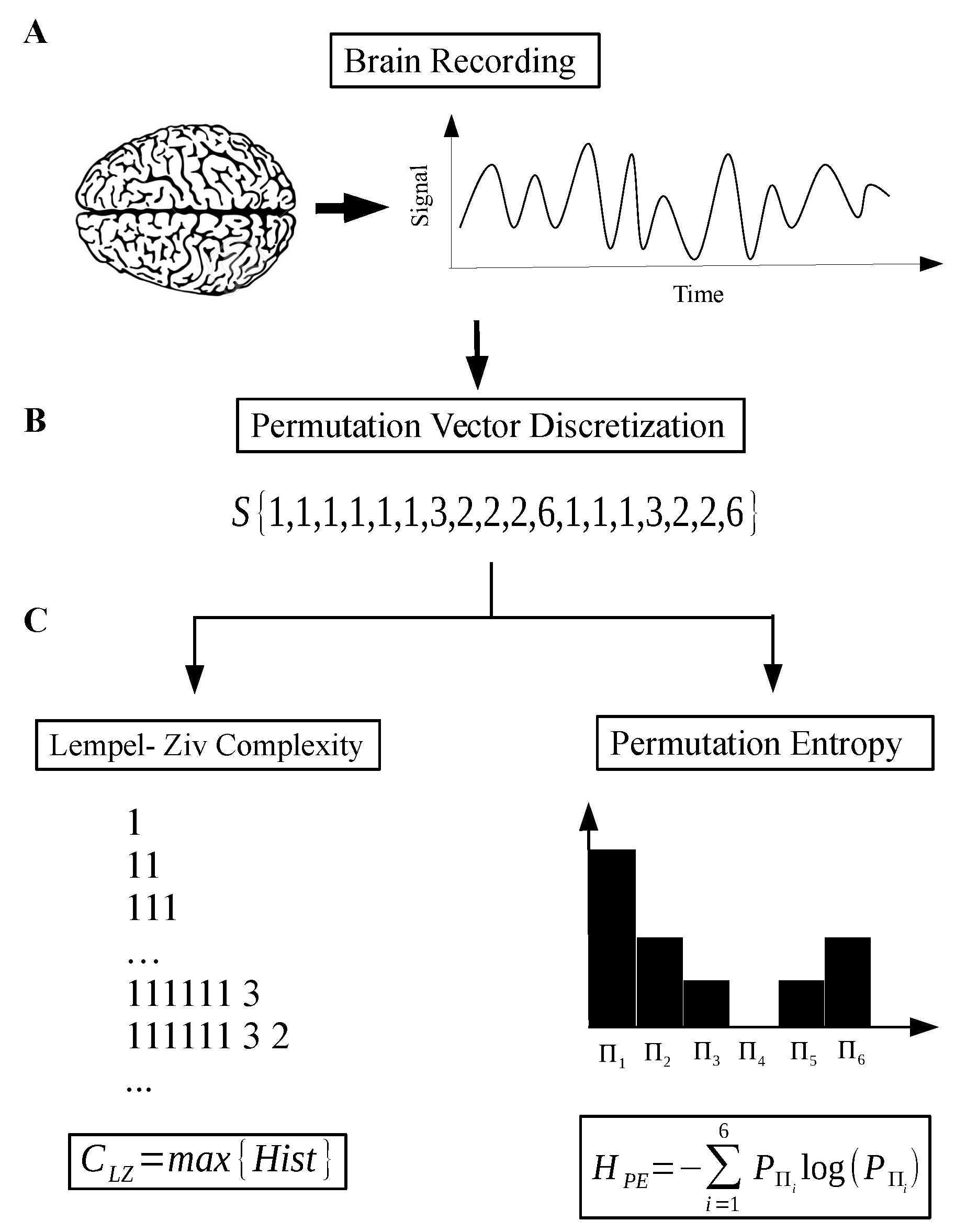
  • Step 1: Record and reprocess the signal—using band pass filter and notch filter at 60 Hz (Figure 2A).
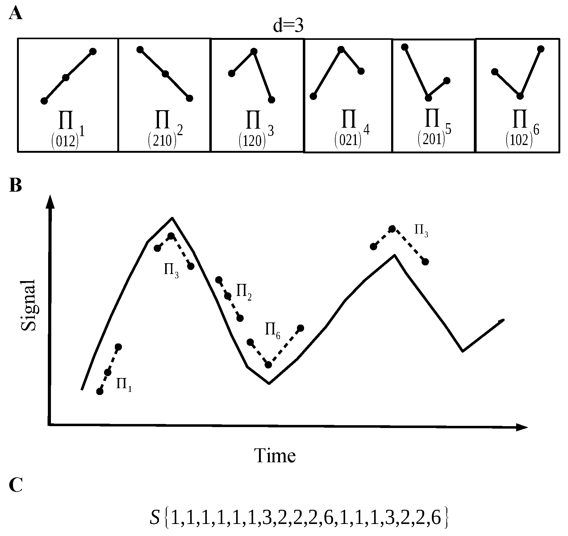
  • Step 2: Discretize the raw signal using a permutation vector approach (Figure 2B).
  • Step 3: Calculate the Lempel–Ziv complexity for the sequence taken from step 2 (Figure 2C).
  • Step 4: Take the sequence from step 2 and, using a histogram, estimate the probability distribution (PD) of permutation vectors. Then, calculate the Shannon entropy related with this PD.
  • Step 5: Finally, with the two measures, we have the coordinates ( h P E , C L Z ) of the map corresponding to the recorded signal.
To make a statistical analysis, for example, determine the mean value and standard deviation of different channels, or, for a group of people, it is required to calculate the covariance matrix Σ h , c . For a group of measure h P E { h 1 , , h n } and C L Z { c 1 , , c n } . The matrix entries are given by:
Σ i , j = E [ ( h i μ c ) ( c i μ h ) ] i , j = 1 , , n ,
where E is the expectation value and μ c , μ h are the mean value of the entropy and the complexity, respectively.

2.2. Patient Recording

The present work has a comparative, observational and retrospective design between a control group versus two clinical cases of patients with diagnosed pathologies, who were studied and followed for more than one year of evolution in a laboratory of clinical neurophysiology. During the study period, the patients with diagnosed pathologies followed the therapeutic indications of their treating physician and electroencephalographic studies were carried out in different instances of their treatment. In both cases, these patients were undergoing treatment with psychotropic drugs. The electroencephalographic studies were analyzed retrospectively and compared to the parameters obtained after applying the same methods to the control group.

Technical Procedures and Clinical Description

For the conformation of the control group, N = 20 EEG recordings were selected from a database of a clinical neurophysiology laboratory (IACCo). Inclusion–exclusion criteria were: (a) the records should be adult individuals (18–50 years) with no medical history; (b) the individuals should not be taking psychotropic medication at the time of the study; (c) the study should be performed without facilitator medication like chloral hydrate and/or similar; (d) EEG records have to be reported as normal pathways by the specialist physician; (e) records should not contain non-physiological artifacts; (f) studies that conformed to the control group should have a similar duration; (h) the studies of the control group should be performed under equal conditions (closed eyes and similar number of samples and electrodes) than the pathological cases studied.
Each record analyzed here was performed according to the standards of the International Federation of Clinical Neurophysiology [20], following the international system 10–20 for the placement of electrodes. The records are presented in monopolar montages, with bimastoid reference for a total of 20 channels. The signal was taken with a low resolution sampling of 65 Hz, with conventional hospital use equipment, according to local regulations. The number of individuals was N = 20 and the mean age was 33 ± 10 of both sexes and the duration of the records was 37 ± 9 min for all cases in the control group. All of the information about the Control group is summarized in Table 1.

2.3. Clinical Description of the Cases

2.3.1. Case I

The records in this case correspond to a 22-year-old female patient whose clinical diagnosis was Idiopathic Generalized Epilepsy (ICD-10 G 40.3). She had clinical follow-up for a period of two years. During this time, four EEG recordings were performed. The references of these studies will be T 0 , T 1 , T 2 and T 3 , respecting the chronological order in which they were realized.
The initial condition from which the case description starts is T 0 . The study was performed when the patient was taking 1200 mg/day of carbamazepine, without any improvement. The situation led to an average of 10 seizures per week. After her first EEG recording ( T 0 ), the pharmacological scheme was changed to carbamazepine 400 mg/day and valproic acid 1000 mg/day. The change improved the clinical state and the number of seizures reduced to two per month. The improvement persisted throughout the first year of follow-up, and it is reflected in the following EEG recording T 1 taken 10 months after T 0 . Immediately after T 1 , a new pharmacological scheme was implemented, including Lamotrigine 400 mg/day and 1500 mg/day of Levetiracetam. The change brought the seizure frequency to a seizure every three months. After seven months of the new pharmacological scheme, T 2 was recorded. The latter improvement observed in the clinic could not be discriminated by the method of visual inspection of the signal, and the neurophysiological report of T 2 was described as an evolution without significant changes. At this point, the dose of one of the drugs of the last implemented scheme was increased, that is, Levetiracetam 2000 mg/day and maintaining Lamotrigine 400 mg/day. After the change, the patient remained for more than six months without any seizures. Seven months later, T 3 was recorded. The time elapsed between T 0 and T 3 is approximately two years of treatment. In all studies, there were no seizures during the recording, so the tracings correspond to intercritical records.
Electroencephalographic records in Figure 3 were reported as: T 0 , severe Bilateral Disorganization; T 1 and T 2 records were reported as moderate Bilateral Disorganization, in which no significant differences were found between both registries and a favorable evolution between both in comparison with T 0 . The last one, T 3 , was described as a Bilateral Disorganization leading to frontal predominance, with a significant improvement in relation to the previous tracings.

2.3.2. Case II

The second case corresponds to a 41-year-old man diagnosed with narcolepsy ( CIE-10 G47.4) and morbid obesity as co-morbidity. In this case, three follow-up studies were made, namely T 0 , T 1 and T 2 in an overall period of 16 months. Again, the subindexes represent the chronological order in which the studies were performed.
At the initial condition T 0 , the patient was medicated with Topiramate 250 mg/day because of his eating disorder. However, the medication provoked no changes in symptoms related with narcolepsy. After T 0 , the pharmacological scheme was changed and Modafinil 200 mg/day was added. After nine months with the new scheme (Topiramate 250 mg/day, plus Modafinil 200 mg/day), a clinically significant change was achieved in relation to nocturnal rest and a marked decrease in daytime sleepiness, which also improved the patient’s performance in daily life activities. At this point, T 1 was recorded and no pharmacological changes were introduced. Seven months later, T 2 was performed just to check the evolution of the patient. In this last evaluation, the recording time was doubled in order to record sleep activity in the EEG. Nevertheless, the patient remained awake with his eyes closed during the two hours of the study. As expected from its favorable evolution, daytime sleepiness continued to decline as treatment time advanced.
The electroencephalographic records in Figure 4, T 0 were reported as a Severe Sleep Cycle-Vigil Disorder with a Normal Vigil plot. Here (Figure 4A), K complexes and sleep spindles can be observed, which are characteristic of Phase II, non-Rapid eye movement (non-REM) sleep. These patterns are best presented at the electrodes near the electrode C z . In T 1 (Figure 4B) and T 2 (Figure 4C), tracings were reported as tracings within normal limits. In the retrospective evaluation between the T 1 and T 2 , no significant clinical differences were found. Both traces correspond to closed eyes awake records.

3. Results

We analyze our two specific cases and each of the 20 subjects that conform to the control group explained in Section 2.2. We analyze the EEGs under the Permutation Entropy (PE) and the Permutation Lempel–Ziv complexity (PLZC), using the same permutation vector parameters. The data were preprocessed with the usual removal of signal artifacts and application of band pass filters [0.5, 45] Hz, prior to applying our method.
Every EEG channel was analyzed separately and using the whole recording. The results were presented in a complexity–entropy map. The parameters used for the permutation quantification were d = 3 , 4 , 5 , 6 and τ = 1 , giving similar results (for different d, the absolute value of HPE and PLZC is not the same, but the relative values between them were almost similar). The center of the ellipse corresponds to the mean value of the corresponding studies of the control group, and the ellipse itself to the joint error of PE and PLZC of this group. The values of embedding (d) were chosen since they are suggested in most of the literature about PE analysis for EEG signal analysis [3,21]. For the τ value, we consider a study of PE done in the Rossler, Lorenz and B attractor [22], in which the authors emphasize that when the signal has large lag time, the correlation between the signals is lost, with low values of τ being the best option. Because our sampling frequency is low, we choose to use τ = 1 .
Regarding our first patient (case I, see Section 2.2), Figure 5 shows the results of the four EEG monitoring sessions performed in an evolutionary follow-up of a 22-year-old woman diagnosed with Generalized Idiopathic Epilepsy. Here, a clear displacement in the plane between the T 0 and T 1 is observed. The interval between the two studies was 10 months, and it corresponds to a large decrease in the frequency of seizures.
The time elapsed between T 1 and T 2 was seven months. This corresponds to the change in the pharmacological scheme that sought to prevent the patient from having seizures, not only to reduce their frequency. Here, the neurophysiological report of the electroencephalogram by visual inspection found no significant change between them. However, there was an improvement in the clinical aspect of the condition. Finally, in T 3 , the optimization of the pharmacological scheme used until T 2 can be observed. This achieves a new significant change both in the clinical aspect and in the electroencephalographic tracing. This can be seen in the approaching, in many channels to the center of the ellipse, that corresponds to the mean value of the studies of the control group.
Figure 6 (case II, see Section 2.2) shows the results of the evolutionary follow-up of a 41-year-old male with a diagnosis of narcolepsy and morbid obesity. Here, the three electroencephalographic monitoring sessions can be observed, comparing the differences between the abnormal study T 0 (Severe Sleep Cycle-Vigil Disorder) with T 1 and T 2 , which are reported as normal. However, between T 1 and T 2 , there is little difference: T 1 lasted one hour and T 2 lasted two hours with a previous sleep deprivation. Calculations for T 2 were analyzed for each hour separately and similar results were found between the two halves, so the graph shows the values of the complete study (2 h). It is also possible to identify that the values of the plane for the study T 0 are lower in the electrodes near C z .

4. Discussion

The results allow us to compare the values obtained for each channel of an EEG, with the mean value of the control group and the corresponding error (ellipse). These give global information about the signal, supplementing the traditional method of visual inspection of EEG, which is usually performed on a time scale of a few seconds and whose reading is done sequentially.
In the first case, the map is used as a tool that allows us to show the effectivity of pharmacological treatment in patients treated with psychotropic drugs. In a pathology such as epilepsy, the EEG signal tends to be more regular. This regularity gives less number of different permutation vectors and it provokes a decrease in the entropy and complexity values. Similar results were shown comparing awake people with people in altered states of consciousness such as sleep, seizures, and comas [19]. Analogous results are shown in other epilepsy syndromes, such as absence crises [23]. In our first case, although there is an interelectrode difference that can be observed in the plane, there is evidence of a common trend in all channels—the pathological values approach to the control group, reflecting a change in the functional state of the nervous system that correlates with the favorable evolution after each pharmacological intervention. Moreover, when the visual inspection method of EEG did not show significant changes between the T 1 and T 2 studies, the pharmacological scheme was changed and it corresponded to an improvement in the clinic. The complexity–entropy plane was able to detect such a change from the global evaluation of the entire record for each electrode. As it can be seen in Figure 5 and Figure 6, the nine channels showed smaller distances to the center of the ellipse in T 2 compared with T 1 . This subtlety, which had clinical value, could not be detected by the human eye. In addition, by optimizing the dose, a major change was achieved, and it is visible in T 3 . EEG records in epilepsy are now described as critical and intercritical records. However, most of the studies that are done in clinical practice are intercritical records because there is no way to predict a seizure and only in some cases can the crises be reproduced. The cases are those that respond to sensitization methods, such as intermittent light stimulation, and usually they have a genetic or syndromic association that is still unknown [24]. Therefore, a quantitative evaluation of the intercritical records opens the possibility of comparing studies, in which it is not possible to perform a semiologic description of the seizure, but from which it is possible to obtain valuable information about the clinical evolution of the epileptic patient.
In the second case, which corresponds to the 41-year-old patient with narcolepsy, the CLZ vs. HPE method of analysis is also used. It should be recalled that the EEG sleep pattern is different from the awake pattern, and these differences in paths are observed by the visual inspection method (Figure 4) and also identified by the CLZ vs. HPE plane. In the images of T 0 in Figure 4, some patterns of the characteristic pattern of non-REM sleep phase 2 such as K-complexes and spindles [25,26] can be found. During this study, the patient was able to maintain the waking state during very short periods of time and most of the EEG tracing corresponds to a sleep pattern. Here, PCLZ vs. HPE values are very low values for most electrodes; nonetheless, in daily clinical practice, low values in the plane are unusual for short studies, since most patients usually maintain a vigil or enter a light sleep state in records of an hour or less duration. This is related to the low values found in individuals with altered states of consciousness such as those presented in [19].
After the administration of Modafinil, the tracings present normal patterns of the vigil state with closed eyes. In Figure 4, segments of these studies are shown and correspond to T 1 and T 2 . The values found in the PCLZ vs. HPE plane for such studies are similar to the values found in control individuals.
The similarity of these values in both studies correspond to the fact that the patient treated with Modafinil managed to stay awake during the whole records. In the channels F3–C3–F4–C4–F8 of Figure 6, it is possible to observe the small difference between the values obtained in the plane for the T 1 and T 2 studies. Note that the time elapsed between these studies is seven months and T 2 is twice as long as T 1 . The approximation of the values of both studies to the center of the ellipse shows an improvement of the patient with respect to T 0 . The fact that there is a proximity in the values of the channels between the two studies ( T 1 and T 2 ) indicates a certain stability in the improvement, which correlates to the clinical evolution that the picture had.
Note that, in this work, low values in the plane correspond to pathological clinical conditions or changes in the state of consciousness. [19,23]. For example, as shown in the first case, the low values correspond to changes found in the signal given by patterns (graphs) of pathological discharges in intercritical studies of a patient with epilepsy. However, in the second case, in the EEG, there are pathological patterns (graphemes), but there are not physiological patterns of normal sleep that should not appear in a closed-eyes waking study if the patient could maintain alertness during a short duration EEG and without facilitating medication.
In this way, the PCLZ vs. HPE map would provide new information to methods like MSLT (the Multiple Sleep Latency Test) and polysomnography for the evolutionary and/or diagnostic studies of narcolepsy. In addition, as shown in case I, the evolutionary study of patients with neuropsychiatric pathologies, relevant information is provided by the plane. This is found by the fact that there is an individual variation in the response to psychotropics, an aspect that, if taken into account, would achieve in the future the development of a more personalized drug therapy.

5. Conclusions

In this work, we show one application of the “PLZC vs. HPE” map for electroencephalographic interpretation in clinical neurophysiology. This method allows us to look at the changes that occur in long-term treatments from a single perspective, something that the method of visual inspection can not provide. We have applied the analysis to a control group in order to have a statistical reference. In a dynamic interpretation of the results, we find that, for healthy people, the permutation entropy and permutation Lempel–Ziv complexity tend to be at a maximum, decreasing when the person has a pathology. This is because, for a normal awake state, the EEG signal tends to be similar to a discorrelate white noise [27], which has the highest entropy and complexity [19].
The instrument presented here has been used as a global assessment tool, sacrificing short-term signal changes, that is, its non-stationary behavior. However, we could see that reducing the signal length to 10 min shows that the results do not vary widely. It is also possible to apply the instrument with smaller sliding windows and retrieve this information if it is considered relevant as done in [19]. The method also allows one to compute the entropy and complexity of a signal using just the waveform of the EEG. Because of this, it is not necessary to select a specific band frequency for the analysis; the information that we obtain from the signal is more robust (nevertheless, this does not limit the application of the method to particular frequency bands). The visualization of the data in a complexity–entropy graph permits a better understanding of the results especially for people who are not so familiar with this kind of analysis. The method is very simple to apply and has a very low computational cost, which makes it very appropriate for real-time analysis. The method has no limitations to the length of recording, although it is very important to take into account the parameters used for the analysis, especially the embedding dimension d. As an additional feature, the analysis was done for each channel separately; thus, it can be used in different types of recording settings.
Taking up the clinical objectives of this work, we consider that the instrument is useful for the evolutionary follow-up of patients undergoing pharmacological treatment with psychotropic drugs. The epidemiological and statistical approach in electroencephalography is accessible if the control groups can be adjusted by age groups, the latter being especially important in neonatal electroencephalography. For prolonged studies of hours or days of patients hospitalized in electroencephalographic monitoring units, the instrument offers the possibility of reading each recorded signal hourly, which helps to reduce the reading time of such monitoring in medical care tasks.
Finally, in relation to pharmacodynamic studies by means of EEG signals, the spectrogram is one of the most widely used methods in the field of anesthesiology. The instrument presented here was not used for this purpose. However, we think that it can add information to the data obtained by the spectrogram and contribute to the investigation in this field. This is part of the work in progress.

Acknowledgments

The authors thank the Directors of IACCo, Graciela Lucatelli and Atilio Bollo for the support received for this work. They also thank Pedro Lamberti for useful discussions.

Author Contributions

Juan M. Diaz did the EEG recordings and conducted the neurophysiological evaluations of the data. Diego M. Mateos did the calculations, data analysis and graphs. Dra Carina Boyallian discussed the results. All authors participated in the manuscript writing and approved the final version.

Conflicts of Interest

The authors declare no conflict of interest.

References

  1. Janáčková, S.; Boyd, S.; Yozawitz, E.; Tsuchida, T.; Lamblin, M.D.; Gueden, S.; Pressler, R. Electroencephalographic characteristics of epileptic seizures in preterm neonates. Clin. Neurophysiol. 2016, 127, 2721–2727. [Google Scholar] [CrossRef] [PubMed]
  2. Purdon, P.L.; Pierce, E.T.; Mukamel, E.A.; Prerau, M.J.; Walsh, J.L.; Wong, K.F.K.; Salazar-Gomez, A.F.; Harrell, P.G.; Sampson, A.L.; Cimenser, A.; et al. Electroencephalogram signatures of loss and recovery of consciousness from propofol. Proc. Natl. Acad. Sci. USA 2013, 110, E1142–E1151. [Google Scholar] [CrossRef] [PubMed]
  3. Olofsen, E.; Sleigh, J.; Dahan, A. Permutation entropy of the electroencephalogram: A measure of anaesthetic drug effect. Br. J. Anaesth. 2008, 101, 810–821. [Google Scholar] [CrossRef] [PubMed]
  4. Bandt, C.; Pompe, B. Permutation Entropy: A Natural Complexity Measure for Time Series. Phys. Rev. Lett. 2002, 88, 174102. [Google Scholar] [CrossRef] [PubMed]
  5. Zozor, S.; Mateos, D.; Lamberti, P.W. Mixing Bandt-Pompe and Lempel-Ziv approaches: Another way to analyze the complexity of continuous-states sequences. Eur. Phys. J. B 2014, 87, 107. [Google Scholar] [CrossRef]
  6. Jung, T.P.; Makeig, S.; Stensmo, M.; Sejnowski, T.J. Estimating alertness from the EEG power spectrum. IEEE Trans. Biomed. Eng. 1997, 44, 60–69. [Google Scholar] [CrossRef] [PubMed]
  7. Adeli, H.; Zhou, Z.; Dadmehr, N. Analysis of EEG records in an epileptic patient using wavelet transform. J. Neurosci. Methods 2003, 123, 69–87. [Google Scholar] [CrossRef]
  8. Rosso, O.; Larrondo, H.; Martin, M.; Plastino, A.; Fuentes, M. Distinguishing noise from chaos. Phys. Rev. Lett. 2007, 99, 154102. [Google Scholar] [CrossRef] [PubMed]
  9. Rosso, O.A.; Craig, H.; Moscato, P. Shakespeare and other English Renaissance authors as characterized by Information Theory complexity quantifiers. Physica A 2009, 388, 916–926. [Google Scholar] [CrossRef]
  10. Montani, F.; Rosso, O.A. Entropy-Complexity Characterization of Brain Development in Chickens. Entropy 2014, 16, 4677–4692. [Google Scholar] [CrossRef]
  11. Mateos, D.M.; Zozor, S.; Olivarez, F. On the Analysis of Signals in a Permutation Lempel–Ziv Complexity-Permutation Shannon Entropy Plane. arXiv 2017, arXiv:1707.05164. [Google Scholar]
  12. Cover, T.M.; Thomas, J.A. Elements of Information Theory, 2nd ed.; John Wiley & Sons: Hoboken, NJ, USA, 2006. [Google Scholar]
  13. Thakor, N.V.; Zhu, Y.S.; Pan, K.Y. Ventricular Tachycardia and Fibrillation Detection by a Sequantial Hypothesis Testing Algorithm. IEEE Trans. Biomed. Eng. 1990, 37, 837–843. [Google Scholar] [CrossRef] [PubMed]
  14. Zhang, X.S.; Zhu, Y.S.; Thakor, N.V.; Wang, Z.Z. Detecting ventricular tachycardia and fibrillation by complexity measure. IEEE Trans. Biomed. Eng. 1999, 46, 548–555. [Google Scholar] [CrossRef] [PubMed]
  15. Radhakrishnan, N.; Gangadhar, B.N. Estimating Regularity in Epileptic Seizure Time-Series Data—A Complexity-Measure Approach. IEEE Eng. Med. Biol. Mag. 1998, 17, 89–94. [Google Scholar] [CrossRef] [PubMed]
  16. Hansel, G. Estimation of the entropy by the Lempel-Ziv method. In Lecture Notes in Computer Science (Electronic Dictionaries and Automata in Computational Linguistics); Springer: Berlin/Heidelberg, Germany, 1987; Volume 377, pp. 51–65. Available online: https://link.springer.com/chapter/10.1007/3-540-51465-1_4 (accessed on 13 October 2017).
  17. Schürmann, T.; Grassberger, P. Entropy estimation of symbol sequences. Chaos 1996, 6, 414. [Google Scholar] [CrossRef] [PubMed]
  18. Amigo, J.; Kennel, M.B. Variance estimators for the Lempel-Ziv entropy rate estimator. Chaos 2006, 16. [Google Scholar] [CrossRef] [PubMed]
  19. Mateos, D.; Erra, R.G.; Wennberg, R.; Velazquez, J. Measures of Entropy and Complexity in Altered States of Consciousness. arXiv 2017, arXiv:1701.07061. [Google Scholar]
  20. Deuschl, G.; Eisen, A.; International Federation of Clinical Neurophysiology; International Federation of Societies for Electroencephalography and Clinical Neurophysiology. Recommendations for the Practice of Clinical Neurophysiology: Guidelines of the International Federation of Clinical Neurophysiology. 1999. Available online: http://www.clinph-journal.com/content/guidelinesIFCN (accessed on 13 October 2017).
  21. Popov, A.; Avilov, O.; Kanaykin, O. Permutation entropy of EEG signals for different sampling rate and time lag combinations. In Proceedings of the Signal Processing Symposium (SPS), Serock, Poland, 5–7 June 2013; pp. 1–4. [Google Scholar]
  22. De Micco, L.; Fernández, J.G.; Larrondo, H.A.; Plastino, A.; Rosso, O.A. Sampling period, statistical complexity, and chaotic attractors. Physica A 2012, 391, 2564–2575. [Google Scholar] [CrossRef]
  23. Mammone, N.; Duun-Henriksen, J.; Kjaer, T.W.; Morabito, F.C. Differentiating interictal and ictal states in childhood absence epilepsy through permutation Rényi entropy. Entropy 2015, 17, 4627–4643. [Google Scholar] [CrossRef]
  24. Taylor, I.; Marini, C.; Johnson, M.R.; Turner, S.; Berkovic, S.F.; Scheffer, I.E. Juvenile myoclonic epilepsy and idiopathic photosensitive occipital lobe epilepsy: Is there overlap? Brain 2004, 127, 1878–1886. [Google Scholar] [CrossRef] [PubMed]
  25. Kryger, M.; Roth, T.; Dement, W. Principles and Practice of Sleep Medicine; Elsevier: Amsterdam, The Netherlands, 2017; pp. 1592–1601. [Google Scholar]
  26. Goldman, L.; Bennett, J.C. Tratado De Medicina Interna; Macgraw-Hill: New York, NY, USA, 2002. [Google Scholar]
  27. Bandt, C. A New Kind of Permutation Entropy Used to Classify Sleep Stages from Invisible EEG Microstructure. Entropy 2017, 19, 197. [Google Scholar] [CrossRef]
Figure 1. Example of the permutation vector discretization. (A) for the parameter d = 3 , we have d! = 6 possible patterns; (B) to each data point t = 1 , , n ( d 1 ) is assigned the corresponding pattern, depending on the relative values of the neighbors; (C) the quantified sequence to the original signal.
Entropy 19 00540 g001
Figure 2. The steps to analyze a recording signal through the Complexity vs. Entropy map. (A) signal recording and preprocessing; (B) quantify the signal using the permutation vector approach; (C) calculate the permutation Lempel–Ziv complexity and the permutation entropy for the quantify sequence.
Entropy 19 00540 g002
Figure 3. EEG recording for the four states of treatment (Case I). (A) T 0 corresponds to the first monitoring performed, and it can be observed that before the time 5:52 and after the time 5:55, the discharges occur in both hemispheres and had a duration greater than 10 s. (B,C) In the studies T 1 and T 2 , bilateral short-term discharges of 2–3 s are observed. There is little clinical differentiation between studies T 1 and T 2 . (D) In the study T 3 , a trace with a normal voltage with a predominance of bilateral slow rhythms in the frequency domain is observed. All studies correspond to intercritical records.
Entropy 19 00540 g003
Figure 4. EEG traces belonging to patient diagnosed with narcolepsy (Case II). (A,B) T 0 corresponds to sleep paths, and in both can see the slow waves between 3 and 5 Hz. In addition, K and spindle complexes, characteristic of phase 2 of non-REM sleep, are observed. (C,D) The T 1 and T 2 traces correspond to normal records in the waking eyes closed condition. T 2 trace corresponds to the second hour of the monitoring. A trace of low voltage with alpha and theta rhythms is observed in both records.
Entropy 19 00540 g004
Figure 5. PLZC vs. HPE map analysis belonging to a patient diagnosed with Generalized Idiopathic Epilepsy, in four different stages of treatment (square and triangles), compared to the mean value of a control group and their respective errors (circle and ellipse). Each subplot shows the analysis for a particular EEG channel (despite starting in the inner plot). The parameters used were d = 4 and τ = 1 .
Entropy 19 00540 g005
Figure 6. PLZC vs. HPE map analysis belonging to a patient diagnosed with generalized narcolepsy, in three different stages of treatment (square and triangles), compared to the mean value of a control group and their respective errors (circle and ellipse). Each subplot shows the analysis for a particular EEG channel (despite starting in the inner plot). The parameters used were d = 4 and τ = 1 .
Entropy 19 00540 g006
Table 1. Control group information.
SubjectTime Record (MIN)Segment Time Analyzed (MIN)GenderAge
16044M24
26049M20
36044M31
46044M48
56044M25
66048M38
73030F27
83030F28
93030M19
106030F32
113030F44
123025F40
133025F38
146048M48
156039M34
166050M50
176040M23
183030M23
196041M31
206045F27

