A Behavioural Analysis of Complexity in Socio-Technical Systems under Tension Modelled by Petri Nets


Faculty of Economics and Administration, Institute of System Engineering and Informatics, University of Pardubice, 532 10 Pardubice II, Czech Republic
*
Author to whom correspondence should be addressed.
Entropy 2017, 19(11), 572; https://doi.org/10.3390/e19110572
Submission received: 14 September 2017
/
Revised: 19 October 2017
/
Accepted: 20 October 2017
/
Published: 25 October 2017
(This article belongs to the Special Issue Entropy and Its Applications across Disciplines)
Abstract
:Complexity analysis of dynamic systems provides a better understanding of the internal behaviours that are associated with tension and efficiency, which in the socio-technical systems may lead to innovation. One of the popular approaches for the assessment of complexity is associated with self-similarity. The dynamic component of dynamic systems represents the relationships and interactions among the inner elements (and its surroundings) and fully describes its behaviour. The approach used in this work addresses complexity analysis in terms of system behaviour, i.e., the so-called behavioural analysis of complexity. The self-similarity of a system (structural or behavioural) can be determined, for example, using fractal geometry, whose toolbox provides a number of methods for the measurement of the so-called fractal dimension. Other instruments for measuring the self-similarity in a system, include the Hurst exponent and the framework of complex system theory in general. The approach introduced in this work defines the complexity analysis in a social-technical system under tension. The proposed procedure consists of modelling the key dynamic components of a discrete event dynamic system by any definition of Petri nets. From the stationary probabilities, one can then decide whether the system is self-similar using the abovementioned tools. In addition, the proposed approach allows for finding the critical values (phase transitions) of the analysed systems.
1. Introduction
The complexity analysis of systems is currently a widespread theme. It reflects system features such as comprehensibility, modifiability, uncertainty, or maintainability. These features are especially important during design optimization (e.g., information systems). There are a number of complexity measures that have been defined in a number of areas such as physics, biology, sociology, and others. A brief overview of complexity measures can be found in [1]. In the field of complex systems, exist the so-called phase transitions that change the structural and behavioural properties of the system, and thus its complexity. These changes represent, for example, the change of the information system, change of the top management, etc. The complexity of a system is generally dependent on the degree of its tension that invokes the occurrence of phase transitions and the related qualitative properties, such as efficiency, productivity, sustainability, or adaptability. One of the most widespread examples of complex systems is socio-technical systems that deal with human interaction with technical systems. One of the largest challenges in socio-technical systems is creating an appropriate environment in which the entities show maximum performance without requiring explicit management [2] or that require minimal management. Higher performances of the entities can be achieved through effective management (motivation, reward, tasks, etc.) or with a suitable environment (an environment in which the entities are implicitly motivated towards greater performance—self-imposed tension). An example could be a reward/motivation system for employees in a company, the structure of a workspace, or the flexible system of working hours. Various models for optimal performance are suitable for different types of systems, for example, creative work vs. administrative work. Figure 1 illustrates the general structure of a socio-technical system. Examples of socio-technical systems are workspaces, information systems, organizations, and work teams.
Typically, the issue of optimal management can be summarized as the ability to have the appropriate people at the appropriate time in the appropriate place with the appropriate knowledge and motivation. There are a large number of studies on this issue that are based on the top-down perspective, i.e., the central entity manages the activity of the child entities (contemporary management theories). Currently, the bottom-up approach is becoming increasingly popular, i.e., the entities manage themselves (self-organization). These systems are the main focus of complexity theory, where we comprehend hardly manageable systems as so-called complex systems, i.e., systems with a large number of elements, self-organization, self-similarity at different levels of abstraction, and emergence. With the theory of complex systems is possible to explore arbitrary socio-technical systems from different degrees of imposed tension (e.g., workload, tasks, and mental stress) and analyse their behaviour (e.g., the occurrence of self-similarity or self-organization). The tension can represent the amount of work, tasks, goals, etc. Overall, it is possible to classify three distinct states of each system based on the level of imposed tension (see Figure 2).
Without tension (or with insufficient tension), the system gravitates to the equilibrium state with maximum entropy, i.e., the system is usually dysfunctional or non-flexible. With increasing tension, the system spontaneously tips over into the so-called zone of emergence, in which it starts adaptive processes that ensure optimal efficiency and performance of the system while changing the conditions (environment). Examples of adaptive processes are innovation, patents, increased labour productivity, business process optimization, and optimization of the organizational structure. The transition from the equilibrium (inefficient) zone to the zone of emergence is widely called the edge of order (phase transition, also known as the first critical value). Too much tension can also force the system to become inoperable, because its elements cannot then respond sufficiently in a manner that is quick and efficient, and usually, the system moves to the zone of chaos (deterministic or stochastic) and become dysfunctional. The phase transition that indicates entry of the system into chaotic behaviour is often called the edge of chaos (the second critical value). The amount of tension needed for the occurrence of these phase transitions is variable and depends on the specific system and time. Factors that affect these variables are the motivation, money, environment, ability to work in a team, qualification of personnel, workspace optimization, etc. For example, a high motivation in the employees reduces the amount of tension needed to transition the system into the zone of emergence (edge of order). The higher abilities to work in a team and better organizations of work improve the robustness of the system (increasing the amount of tension that the system is capable of resisting, push the edge of chaos higher). It is apparent that a system should optimally be in the zone of emergence and should have the lowest edge of order and the highest edge of chaos. The aim of this work is to propose an approach (using an analysis of self-similarity) that could determine whether a system with a specific degree of tension is situated in the zone of emergence. It also can find the borders of the zone of emergence (the edge of order and the edge of chaos).
Why is it important to know whether a system is located in the zone of emergence? As mentioned above, a system that is located in this zone is characterized by a number of properties that stimulate creative activities and high motivation of the entities (elements of the system). This state is considered to be desirable, with exceptions, such as strictly hierarchical or bureaucratic systems. Determination of the exact boundaries of the zone of emergence would allow a quantitative assessment about the current robustness of a socio-technical system. Usually, it is preferred to have a system with the first critical value as low as possible because the elements of the system can enter the adaptive zone with a lower amount of imposed tension. This arrangement ensures that the system is flexible enough in the context of a higher-level system (e.g., the flexibility of a company in a competitive market environment). The second critical value should be as high as possible because it ensures maximum system performance without signs of chaotic behaviour. The first critical value represents an existential condition for the development or survival of a specific system in a competitive environment (a value above a certain limit would be destructive), and the second critical value indicates the ability of the system to be the best in the industry (competitive advantage).
The issue of determining whether a system is in the zone of emergence is, in the context of this work, addressed with Petri nets, Markov chains, the Rényi information dimension, and the generalized Hurst exponent. As part of the proposed approach, the considered system is modelled using any type of Petri net (Place Transition Petri nets, Timed Petri nets, Coloured Petri nets, etc.). In the context of this work, the Place Transition (P/T) Petri nets are used. The next step is to determine the stationary probabilities of the individual states (the markings of the Petri net) using an analytical approach that performs a transformation to a Markov chain (for the lower class of Petri nets, e.g., P/T or timed) or using simulation (for the higher class of Petri nets, e.g., Coloured). From the stationary probabilities, we then quantify the Rényi information dimension and the generalized Hurst exponent, from whose mutual relationship a decision is made about the borders (critical values) of the analysed system. Figure 3 briefly represents the chronological process of the present approach.
Currently, the quality of a socio-technical system is judged mostly on its ability to respond to stimuli as soon as possible with the lowest possible cost. The general objective of maximizing the output (e.g., the profit) can lead to a series of unexpected events that are difficult to predict. One such event is the edge of chaos (or any other phase transition in a system), which indicates a quantitative change in the behaviour or structure of a system that could have catastrophic consequences. From biological systems, one can present examples, such as the extinction of a species or a population extinction (e.g., logistic growth with harvesting). In economic systems, the consequences of such quantitative changes would not be very catastrophic, but the psychological problems of workers (susceptibility to error/bad decisions) or dysfunctional workspaces will lead to lower profits or loss of a competitive advantage (in marginal cases, bankruptcy). A field that addresses these issues is, for example, ASM (Abnormal Situation Management).
This article is structured as follows. The second section provides an overview of the current state of all of the areas that are important for the purpose of this article. More specifically, the issue of systems under tension and phase transitions, Petri nets, Hurst exponent, and fractal (information) dimension. The third section contains the formal definition of the proposed approach, which starts with modelling using any definition of Petri nets through the determination of stationary probabilities to the quantification of individual characteristics (the fractal/information dimension and the Hurst exponent). The fourth section provides an example that illustrates the approach of the complexity analysis on a model example. The fifth section discusses the proposed approach, including a summary of its advantages and disadvantages in the context of the current state of this issue. The final chapter summarizes this article and outlines the possible future research in this area.
2. State of the Art
The issue of the appropriate settings for the parameters of a system (or the environment) touches disciplines such as management (social science) and optimization (operational research). Depending on the type and complexity of the system, it is possible to use various methods and models (analytical vs. numerical, deterministic vs. stochastic, etc.). Currently, one of the most popular approaches is the use of agent-based modelling, which is sufficiently robust for the analysis of complex systems. Its disadvantage is an inability to implicitly verify the desired properties of the model and the problematic interpretation of the simulation results. Another popular method that implicitly enable us to verify the properties of the model is the use of Petri nets (see Section 2.4). Their disadvantage is an exponential explosion (of system states), which makes it difficult to analyse larger models. This paper presents an approach based on the analysis of socio-technical systems modelled by Petri nets. A system can be seen from at least two different points of view. The first is the physical or logical structure of the system, which reflects all of the elements of the system and their mutual connections. During the systems analysis, usually the first step is to define all of the entities that the system contains (people, documents, hardware, software, etc.). A second perspective on a system is its behaviour, i.e., its dynamic processes. The structure and behaviour of a system represent its static and dynamic components, and in general, fully describe its existence. This paper works with the second viewpoint. Examples from economic systems are, for example, the one-to-one variable pricing model [4] and activity theory [5]. Examples from the analysis of abnormal situations are issues with humans [6] and the prevention of such situations [7].
The following sections will provide a brief overview of the current state of knowledge in the various areas of interest that are key to the proposed approach.
2.1. System under Tension, Critical Values and Phase Transitions
Usually, tension is imposed on the system to improve its performance [8]. An example of a system can be, for example, a fuel boiler, where every unit of added fuel (at a given time) increases its temperature (performance). However, each system is designed (by its nature or design) to have a certain critical value that when reached, the system can stop (permanently or temporarily) fulfilling the function for which it was designed or is used. For example, a fuel boiler could cause damage or an explosion when a certain high temperature is reached. Systems with a biological component have the advantage that they usually contain a larger number of critical values that they can adopt. In such a system, when a certain critical value is reached, the system changes into a new state (through self-organization), which can better withstand the imposed tension [9]. In general, two types of critical values are used: the first critical value (edge of order) and the second critical value (edge of chaos).
The edge of order (the first critical value) usually represents a situation in which a system leaves the existing order and passes in to a new order, which will comply better with the elements of the system (the system is self-organized to its temporal optimal configuration). An example might be a change to a certain technological process in manufacturing companies because of the inadequacy of the original process or the response of an ecosystem to chemical waste (e.g., a change in the vegetation to a more adaptable species). The first critical value is therefore a point at which the imposed tension is dissolved through self-organization (phase transition to a more appropriate form of order).
The edge of chaos (the second critical value) represents a situation in which a system is no longer capable of dissolving the imposed tension and becomes unusable (e.g., the abovementioned example of the fuel boiler). The system is fading into chaos at this critical point. Between the first and second critical values is the so-called zone of emergence (also called the melting zone), in which the imposed tension initiates an adaptive process, which leads to improved structural and behavioural properties of the system. The region of emergence should be as broad as possible, because the elements of the system have greater space for adaptation (dissipation of the imposed tension). If the system is unable to dissipate the imposed tension, its behaviour becomes chaotic, i.e., the system ceases to fulfil the function for which it was designed. Prigogine and Stengers [10] found that if the energy exchange is balanced and sufficiently intense, a surprising phenomenon occurs, i.e., the system goes to a higher level of complexity. The characteristics of this transition are a crisis of energy exchanges and the random effects of the chaos from the peripheral parts. The system attains new properties, structure, and development. This finding means that all that is known about the system is no longer valid.
2.2. Complexity Measures
Excessive complexity could be a source of vulnerability and could cause reduced profitability or loss of controllability, i.e., a higher complexity relates to a closer position of the system to the edge of chaos, and vice versa. For the purposes of the negation of its impacts, it must be managed, and therefore measured, in the first place. Managing the complexity in systems makes them less vulnerable and more resilient [11]. Over the past ten years, the research area that addresses the measurement of the process of non-functional characteristics has expanded. These non-functional characteristics are, for example, the complexity [12,13], uncertainty [14,15], cohesion [16], and fairness [17]. These characteristics are used for the quantification of the system properties, such as user-friendliness, usability, comprehensibility, and predictability [18]. Complexity measures are historically associated with the analysis of source code [19]. Over time, there developed a pressure for their theoretical and empirical validation [20], which resulted in the improvement of the newly proposed measures. At present, complexity analysis is widely used in connection with business process models [21]. The main common characteristics of complexity measures are their ability to quantify the complexity using a single number that is generally taken from the interval . For example, the analysis of complexity associated with the issue of information systems can be found, for example, in [22,23,24]. Other examples are production [25] or application management [26].
2.3. The Fractal (Information) Dimension
Self-similarity is one of the fundamental features of complex systems. Self-similarity is assessed from the time perspective (autocorrelation) or spatial perspective (the roughness or granularity of a system). Self-similarity in terms of time is usually associated with the analysis of a time series (typically one-dimensional), and the spatial self-similarity is associated with geometric formations, for example, multidimensional rugged objects. Self-similarity can be quantified by using the fractal dimension. A classic Euclidean (integer) dimension represents how many real numbers are needed to describe the specific geometric formation (or the real object). The fractal dimension can be calculated by a number of methods, which historically have originated in the solution of specific issues, for example, the measurement of coastline length [27]. An example might be a method based on a coastal coverage with circles of radius [28], an idea based on the coverage of the coast with a strip of width [29] or an approach working with the term -entropie [30]. Over time, more approaches for determination of the fractal dimension have been defined. A comprehensive overview of the various ways to determine the fractal dimension can be found in [31].
2.4. The Hurst Exponent
The Hurst exponent is used for the analysis of times series with a long memory. Historically, the Hurst exponent was associated with Harold Edwin Hurst, who conducted an analysis of the Nile river, and more accurately, he determined the optimal size for a dam based on historical data of precipitation and drought [32]. In the field of fractal mathematics, this approach was generalized by Benoît Mandelbrot [33], with which he defined a direct relationship to the fractal dimension. The generalized Hurst exponent measures the behavioural randomness of a time series [34]. The values of the Hurst exponent are from the interval <0, 1>, where the values from the interval <0.5, 1> evoke a time series with a long-term positive autocorrelation, and the values from the interval <0, 0.5> evoke a time series in which the values are regularly interspersed between large and small. A Hurst exponent that equals 0.5 represents a non-correlated time series.
The generalized Hurst exponent is defined as Hq, and it is possible to determine it when solving the following equation:
where represents a time delay, represents time, represents the individual values of the time series, and is a constant (real number). An example of the generalized Hurst exponent used for a solution of specific issues is, for example, the scaling of differently developed markets [35] or the monitoring of unstable periods in a financial time series [36].
2.5. Petri Nets
Petri nets are a useful tool for the modelling and analysis of behavioural and structural properties of discrete event dynamic systems. Petri nets were first developed by Carl Adam Petri [38], who sparked their continuous development to the present. Petri nets have been developed for many application, which has led to their specialization for modelling and analysis of specific systems and issues. One of the routes pursuing the development of Petri nets was the definition of new structural and behavioural characteristics that allow for verifying specific properties of the modelled system. Examples of properties that are verified on Petri nets can be liveness, boundedness, reachability, and fairness [39]. Verification of individual properties is usually analytical (for basic classes of Petri nets, e.g., Place Transition Petri nets and Stochastic Petri nets) or based on simulation (for higher classes of Petri nets, e.g., Coloured Petri nets). The other development path has followed the expansion of the basic definition of Petri nets in such a way that their modelling power meets specific requirements. An example would be timed and stochastic Petri nets, which allow for improving the individual state changes by reference to time complexity—deterministically [40,41] or stochastically [42]. Other examples are coloured Petri nets [43,44], which combine Petri nets with another modelling language and thus significantly widen (and mainly simplify) the modelling capabilities of the Petri nets. The main disadvantage of this second path is the fact that the verification options are limited since most of the assumptions (properties) must be determined by using simulation.
3. Proposed Approach
The proposed approach is based on a series of steps that lead first from the modelling of a real system/process with Petri nets, through mapping the Petri net model to a Markov chain and the calculation of the stationary probabilities, to the quantification of the fractal (information) dimension and the Hurst exponent. The following section presents the procedure for the quantification of the abovementioned characteristics together with the restrictions that limit this approach.
3.1. The Quantification of Stationary Probabilities
In the context of this work, an analysis of complexity is presented on the basic definition of Petri nets. In general, the definition of a Petri net can be freely modified (e.g., to higher classes), while the procedure of the complexity analysis remains the same, i.e., the approach is universal to all of the commonly used classes of Petri nets (Place/Transition, Stochastic, Generalized Stochastic, Timed, Coloured, etc.). The first step is the modelling of a specific area in the system using the selected Petri net definition [38]. This step include the classic Place/Transition Petri net [39], timed Petri net [40], stochastic and generalized stochastic Petri net [42] or coloured Petri net [43]. Each definition requires a different approach for the quantification of the stationary probabilities (of individual markings, places or sub-markings), which are the inputs to the second phase of our approach (the second phase is the same for all classes of Petri nets). For the basic Place/Transition, timed and stochastic Petri nets exist an analytical approach for the calculation of stationary probabilities, and for the higher classes (e.g., generalized stochastic Petri nets), simulation must be used to approximate the stationary probabilities. In the following, we present the abbreviated procedure for the quantification of stationary probabilities for Place/Transition Petri net models, which can be found in full in [17]. The procedure for the quantification of the stationary probabilities for stochastic Petri nets can be found in [15].
A generalized Place/Transition Petri net is a 5-tuple, where
- —a finite set of places,
- —a finite set of transitions,
- —places and transition are mutually disjoint sets,
- —a set of edges,
- —a weight function that determines the multiplicity of edges,
- —an initial marking.
Since there is an isomorphic relationship between the state space of the Petri net and a Markov chain [45,46,47], it is possible to perform a mapping from the Petri net terminology to that of Markov chains. The first step in defining the stationary probabilities in Place/Transition Petri nets is the conversion of all reachable markings into the Markov chain. A Petri net in terms of Markov chains can be expressed by using a transition matrix, as follows:
Let be a Place/Transition Petri net, and is its set of all reachable markings. The transition matrix of the is defined as
The transition matrix is a right stochastic matrix, where the individual values correspond to the following rules:
where represents the number of markings that are reachable from . Thus, each branching in the state space is assigned a uniform probability for the different paths. However, it is possible to choose the probability for the different branches explicitly but with the condition .
The stationary probabilities of Place Transition Petri nets are calculated as follows:
Let be a P/T Petri net, and let be its transition matrix. A vector of stationary probabilities is defined as the left Eigenvector of the transition matrix :
The vector then contains the individual stationary probabilities of all reachable markings from :
When calculating the stationary probabilities, it is necessary to analyse the model liveness, since each dead marking corresponds to an absorption state in terms of the Markov chain. Each absorption state can always occur, i.e., its probability is equal to one, and therefore, the stationary probabilities of all other reachable markings are equal to zero.
3.2. The Calculation of the Fractal (Information) Dimension
In this work, the definition of the generalized fractal (information) dimension [48] is used and is defined as follows:
where denotes the distinctive precision, is the probability of the -th marking, and is a constant from the interval . Since the set of all stationary probabilities is finite, it is possible to adjust the definition as follows:
where denotes the number of all reachable markings.
3.3. The Calculation of the Hurst Exponent
As mentioned previously, the Hurst exponent is used for the analysis of time series with a long memory. For the purpose of the proposed approach, in the analysis of complexity, we use the definition of the generalized Hurst exponent (1), which is modified to match the terminology of the generalized fractal dimension. The generalized Hurst exponent is defined for the purpose of this approach as follows:
where is the stationary probability of the i-th place, is the size of the time delay from the interval , where represents the number of all reachable markings, and and are constants. One possible solution for is the application of a logarithm to both sides of Equation (9):
Then, we use a linear regression to determine the slope , from which we obtain the value of the generalized Hurst exponent.
3.4. The Calculation of the Equilibrium
Between the definitions of the generalized fractal (information) dimension and the generalized Hurst exponent exist a direct relationship (2). For self-similar processes, the following equality holds: , which is useful for the purpose of this approach. It simplifies as follows:
The justification is that the stationary probabilities of the individual markings represent a finite set of points, i.e., the 0-dimensional Euclidean space ().
For the calculation of the equilibrium , i.e., the constant from the definition of the generalized Hurst exponent and generalized fractal dimension for which the abovementioned (11) equality holds, we define the following recursive Algorithm 1:
| Algorithm 1 |
This algorithm can be initiated by specifying the default and the change , e.g., , where represents the vector of the stationary probabilities. The algorithm finds the constant to the nearest one-hundredth (it is possible to change the accuracy in the algorithm). The algorithm looks for in the interval .
One can argue that if q is found, than the system exhibits the signs of self-similarity, and thus apply the concepts of complex systems, i.e., the system should be situated in the zone of emergence.
4. Illustration of the Proposed Approach on an Example
In this section, we will illustrate the proposed approach of complexity analysis using a simple example. Figure 4 illustrates an example that could represent a simple business process or a workflow that represents a subset of the behavioural components of a sociotechnical system. The figure can refer to, for example, the processing of an order or invoice, the approval process of loan applications, or logistics.
The example is modelled using the classical Place/Transition Petri net. The following are all of the reachable markings in this model:
| M0 | M1 | M2 | M3 | M4 | M5 | M6 | M7 | M8 | M9 | M10 | M11 | M12 | M13 | |
| P1 | 2 | 1 | 0 | 1 | 1 | 0 | 0 | 1 | 0 | 0 | 0 | 0 | 0 | 0 |
| P2 | 0 | 1 | 2 | 0 | 1 | 1 | 2 | 0 | 0 | 1 | 2 | 0 | 1 | 0 |
| P3 | 0 | 1 | 2 | 0 | 1 | 1 | 2 | 0 | 0 | 1 | 2 | 0 | 1 | 0 |
| P4 | 0 | 1 | 2 | 1 | 0 | 2 | 1 | 0 | 2 | 1 | 0 | 1 | 0 | 0 |
| P5 | 0 | 0 | 0 | 1 | 0 | 1 | 0 | 1 | 2 | 1 | 0 | 2 | 1 | 2 |
| P6 | 0 | 0 | 0 | 0 | 1 | 0 | 1 | 1 | 0 | 1 | 2 | 1 | 2 | 2 |
From all of the reachable markings are quantified their stationary probabilities (using the procedure defined in the previous section). The stationary probabilities of the individual markings for the presented model are as follows:
| M0 | M1 | M2 | M3 | M4 | M5 | M6 | M7 | M8 | M9 | M10 | M11 | M12 | M13 |
| 0.033 | 0.071 | 0.035 | 0.111 | 0.034 | 0.100 | 0.035 | 0.100 | 0.104 | 0.105 | 0.012 | 0.163 | 0.032 | 0.065 |
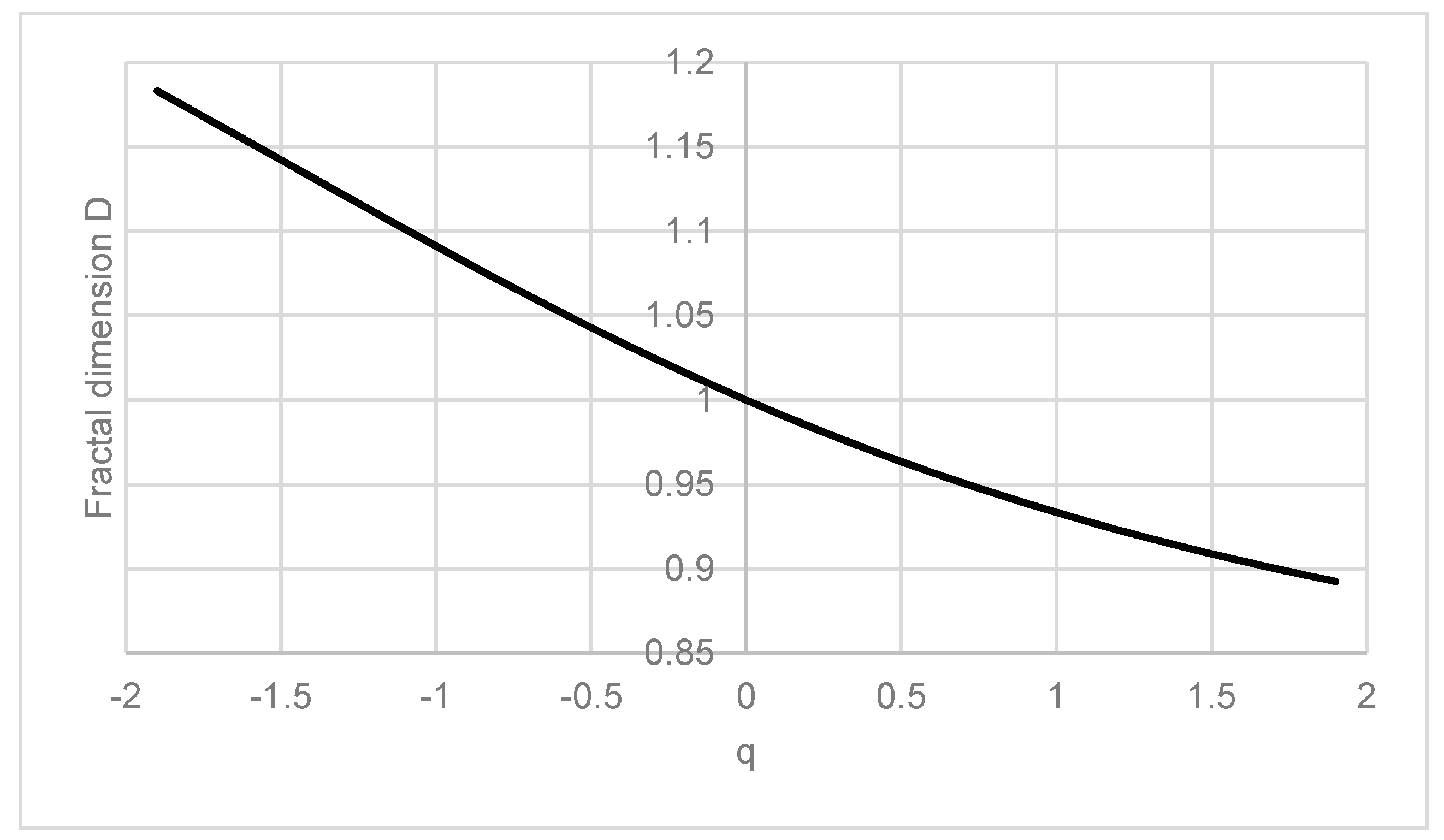
From the calculated stationary probabilities are quantified the essential characteristics that are specific to this approach, i.e., the fractal dimension, the Hurst exponent and the equilibrium . Figure 5 illustrates the size of the generalized fractal (information) dimension depending on the changing constant . The decreasing character of the generalized fractal dimension is given by the growing constant in Equation (9).
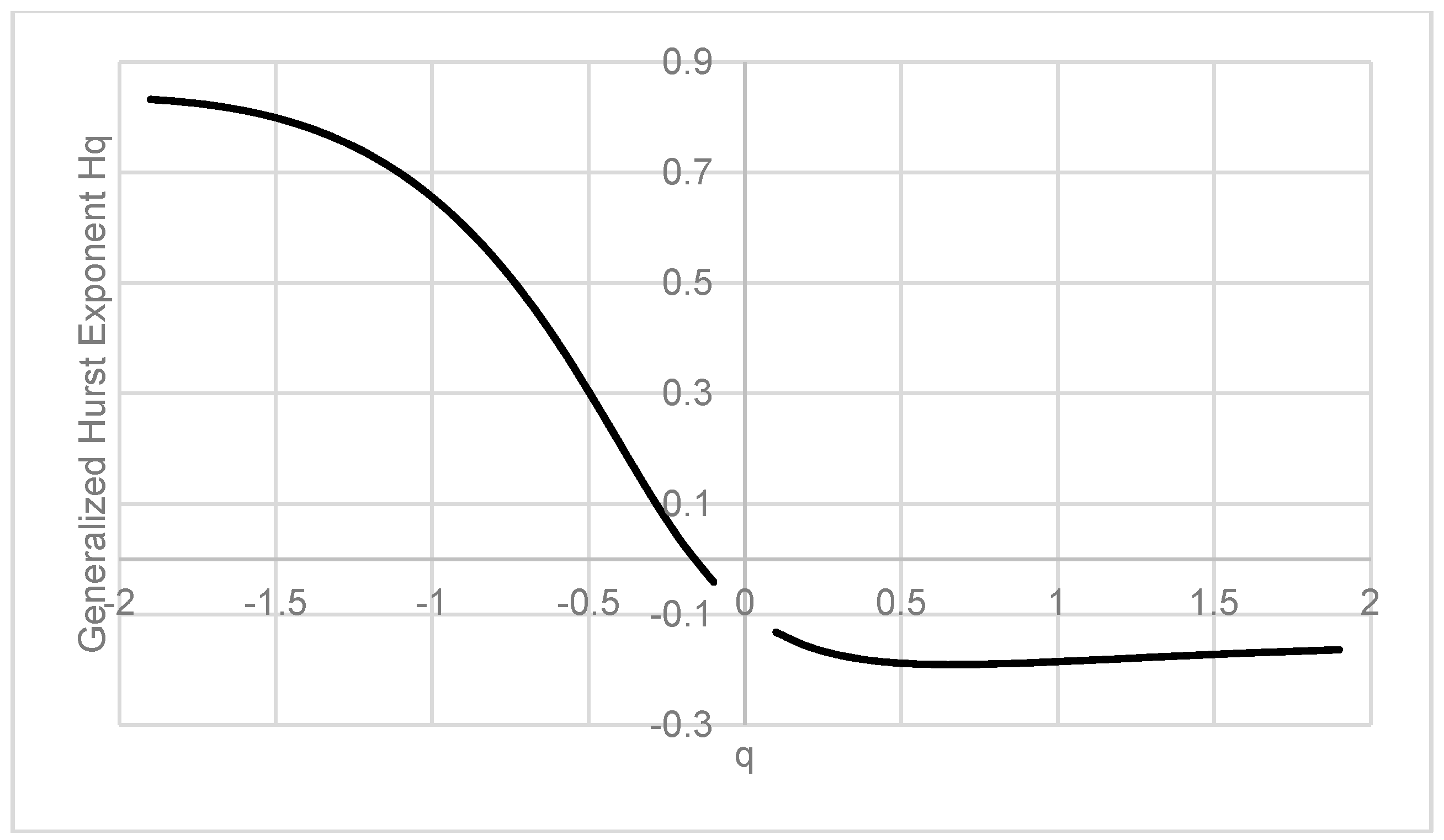
Figure 6 shows the development of the generalized Hurst exponent depending on the constant (the Hurst exponent is not defined for , see Equation (10)).
The subsequent step is to find the equilibrium , for which the equality in (11) holds. Figure 7 illustrates the process of finding the intersection between the generalized fractal dimension and the right side of Equation (11), i.e., . Equilibrium has been found with the use of the abovementioned algorithm for the case , where and . Thus, it can be concluded that the model for two tokens at indicates the signs of self-similarity (since equilibrium was found).
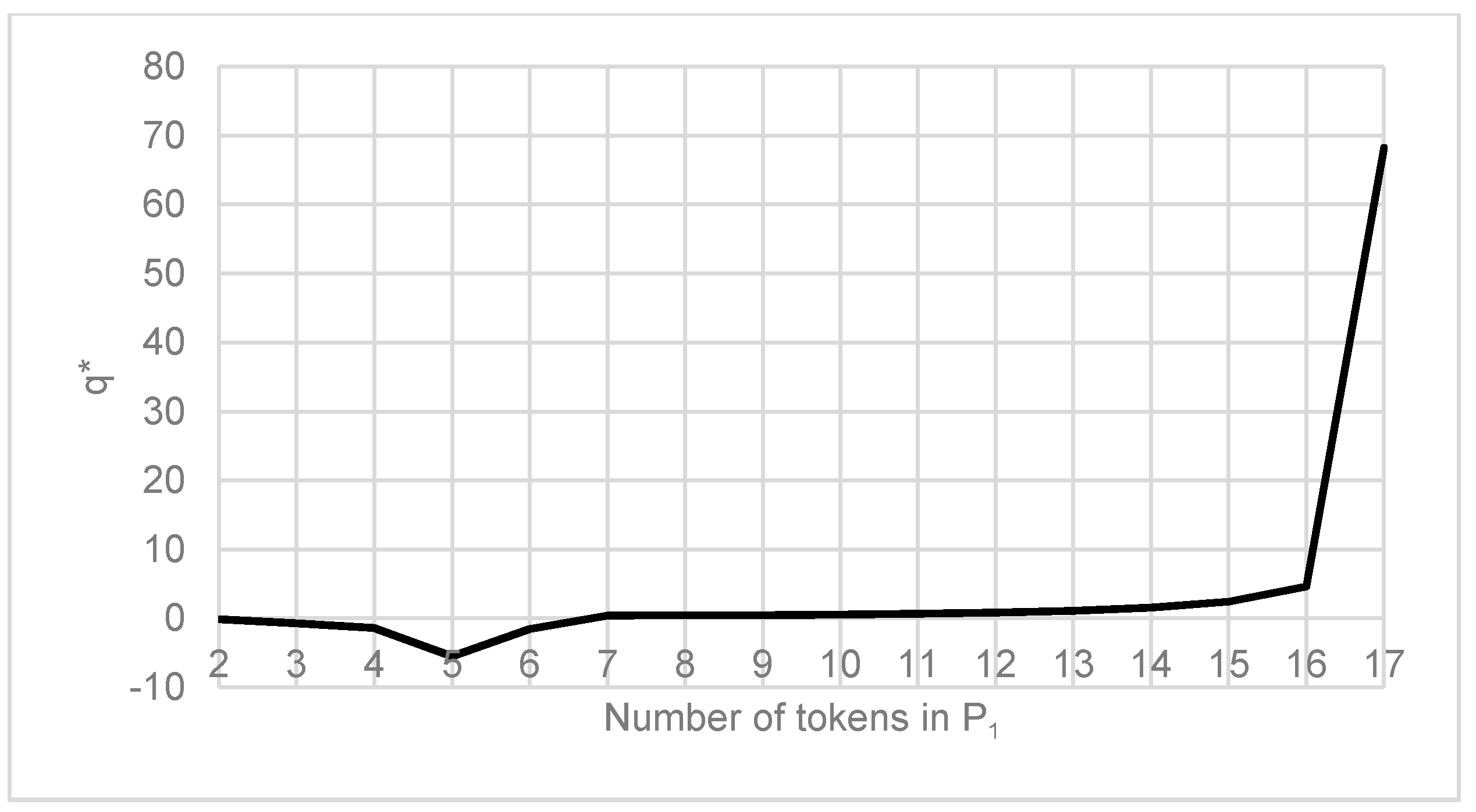
Next, it is possible to perform an analysis of the robustness in terms of self-similarity. Figure 8 shows the evolution of the equilibrium when changing the number of tokens at . The plot contains all of the situations for which the value of was found. In other cases, i.e., if , there are no signs of self-similarity in the model (the equality does not hold, for all ).
These results suggest that the interval corresponds to the zone of emergence in this particular example ( represents the edge of order, and is the edge of chaos).
5. Discussion
Complexity analysis in socio-technical systems provides valuable information about their inner workings. Discrete event dynamic systems are one of the most widespread tools for modelling such systems. A system is usually fully described by its structure and its behaviour. Individual dynamic processes represent the relations and interactions between the various elements of the system (or the surroundings of the system) and fully describe its behaviour. Identification and modelling of these processes are among the most important phases of quality improvement in management and decision making (e.g., for a company).
The approach defined in this work addresses the analysis of sociotechnical systems in terms of their behaviour, i.e., the so-called behavioural analysis of complexity. Individual dynamical processes (e.g., business processes and workflows) and structures can contain repeating patterns, i.e., according to their self-similarity, and we can determine the complexity of a dynamical system. Therefore, the more self-similar the dynamic process is, the greater is its potential for simplification (repeating patterns can be identified and the process adapted), i.e., its complexity can be reduced. The self-similarity of a system (structural or behavioural) can be determined, for example, using fractal geometry, whose toolbox provides a number of methods for the measurement of the so-called fractal dimension. Other instruments for measuring the self-similarity in a system include the Hurst exponent. The other methods for complexity analysis and its comparison are introduced in detail, for example, in our previous work [15].
The dynamic processes that represent the behaviour of sociotechnical systems (or systems in general) in the framework of the proposed approach are modelled using the appropriate class of Petri nets, which constitute a useful tool for the modelling of discrete event dynamic systems. Based on the calculated stationary probabilities (using an analytic approach or simulation) of all of the reachable markings (or sub-markings), it is possible to quantify the abovementioned indicators (the fractal dimension and the Hurst exponent) and decide on the self-similarity of a system. The tool for deciding whether a given system is self-similar is the equality (for a 0-dimensional system with a finite number of configurations). Through finding the equilibrium (see Figure 7), i.e., the constant, , where the abovementioned equality holds, it is possible to conclude that the system exhibits elements of self-similarity.
Finding uses the analysis of the behavioural complexity of sociotechnical systems under tension. The tension in a dynamic process model can be expressed as a number of tokens at key places, and then analysed the development of the equilibrium . It is possible to identify the critical values of the modelled dynamic process where the system begins to show or ceases to show signs of self-similarity (see Figure 8). All of the abovementioned cases have been presented on the simple example.
The advantages of the proposed approach are the following:
- A universal approach for the analysis of the behavioural complexity. Petri nets allow for the modelling of an arbitrary dynamic discrete system. In addition, they have an exact mathematical foundation that allows for verification of a broad number of structural and behavioural characteristics.
- The possibility to analyse the behavioural complexity under tension. The possibility to find the critical values of self-similarity.
The disadvantages of the proposed approach:
- The exponential complexity of the analytical approaches for Petri nets (this shortcoming can be circumvented by simulation).
6. Conclusions
In this work, we have designed an approach that allows for analysing the behavioural complexity in sociotechnical systems under tension. The behavioural complexity is analysed based on self-similarity in the dynamic processes that represent the behaviour of sociotechnical systems. Self-similarity in dynamic processes can be investigated with a number of tools. In this article, self-similarity was analysed using the fractal (information) dimension and the Hurst exponent. Based on the equality in (11), it is possible to determine the equilibrium and decide on the behaviour of a system. If the equilibrium is found, then the system shows signs of self-similarity, and vice versa. Based on this assumption, it is possible to analyse the model under tension and draw conclusions about its behaviour under tension. In this way, it is possible to determine the limits of self-similarity (the minimal and maximal number of tokens at a crucial place for which the system shows signs of self-similarity).
The presented method allows for finding tension limits when the behaviour of the system becomes chaotic. Knowing these limits can enable the optimum process design for the required system tension or for existing process leads to innovations. The presented approach for the analysis of complexity in sociotechnical systems uses modelling with classical Place/Transition Petri nets. The number of tokens on entry to the system represents the tension imposed on the system. The self-similarity of the system has been established while changing the tension in the Petri net model. The presented example has illustrated the approach for complexity analysis in sociotechnical systems under tension.
Future work will focus on the expansion of this approach using other tools that can analyse complexity based on self-similarity or other features (e.g., an attractor in phase space, a disordered state [49] or an agent-based simulation). This approach would ensure that the complexity analysis is more robust (from different points of view) and in the case of agent based simulation also allow to analyse other property of complex systems, the self-organization.
Author Contributions
Martin Ibl and Jan Čapek designed and performed research. Martin Ibl wrote the paper. All authors have read and approved the final manuscript.
Conflicts of Interest
The authors declare no conflict of interest.
References
- Lloyd, S. Measures of complexity: A nonexhaustive list. IEEE Control Syst. 2001, 21, 7–8. [Google Scholar] [CrossRef]
- Nobles, B.; Staley, P. Freedom-Based Management; Freedom, Inc.: Madison, WI, USA, 2010. [Google Scholar]
- Oosthuizen, R.; Pretorius, L. Assessing the impact of new technology on complex sociotechnical systems. S. Afr. J. Ind. Eng. 2016, 27, 15–29. [Google Scholar] [CrossRef]
- Hardaker, G.; Graham, G. Energizing Your E-Commerce through Self-Organising Collaborative Marketing Networks; Technical Report; School of Business, University of Salford: Greater Manchester, UK, 2002. [Google Scholar]
- Vittikh, V.A.; Skobelev, P.O. Multi-agent systems for modelling of self-organization and cooperation processes. WIT Trans. Inf. Commun. Technol. 1998, 20, 24. [Google Scholar]
- Bullemer, P.T.; Dal Vernon, C.R. Managing human reliability: An abnormal situation management historical perspective. In Proceedings of the Mary Kay O’Connor Process Safety Center 2015 International Symposium, College Station, TX, USA, 27–29 October 2015. [Google Scholar]
- Cochran, E.; Nimmo, I. Managing abnormal situations in the process industries I: Automation, people, culture. In Proceedings of the MVMT Workshop, Ann Arbor, MI, USA, 1997. [Google Scholar]
- Tichy, N.M.; Sherman, S. Control Your Destiny or Someone Else Will; HarperBusiness: New York, NY, USA, 2001; xvii; 684p. [Google Scholar]
- Kauffman, S.A. The Origins of Order: Self-Organization and Selection in Evolution; Oxford University Press: New York, NY, USA, 1993; xviii; 709p. [Google Scholar]
- Prigogine, I.; Stengers, I. The End of Certainty: Time, Chaos, and the New Laws of Nature, 1st ed.; Free Press: New York, NY, USA, 1997; ix; 228p. [Google Scholar]
- Leukert, P.; Vollmer, A.; Alliet, B.; Reeves, M. It complexity metrics—How do you measure up? Capco Inst. J. Financ. Transform. 2011, 34, 11–15. [Google Scholar]
- Lassen, K.B.; van der Aalst, W.M.P. Complexity metrics for workflow nets. Inf. Softw. Technol. 2009, 51, 610–626. [Google Scholar] [CrossRef]
- Rolón, E.; Cardoso, J.; García, F.; Ruiz, F.; Piattini, M. Analysis and validation of control-flow complexity measures with bpmn process models. In Enterprise, Business-Process and Information Systems Modeling; Halpin, T., Krogstie, J., Nurcan, S., Proper, E., Schmidt, R., Soffer, P., Ukor, R., Eds.; Springer: Berlin/Heidelberg, Germany, 2009; Volume 29, pp. 58–70. [Google Scholar]
- Jung, J.-Y.; Chin, C.-H.; Cardoso, J. An entropy-based uncertainty measure of process models. Inf. Process. Lett. 2011, 111, 135–141. [Google Scholar] [CrossRef]
- Ibl, M.; Čapek, J. Measure of uncertainty in process models using stochastic petri nets and shannon entropy. Entropy 2016, 18, 33. [Google Scholar] [CrossRef]
- Reijers, H.A.; Vanderfeesten, I.T.P. Cohesion and coupling metrics for workflow process design. In Business Process Management; Desel, J., Pernici, B., Weske, M., Eds.; Springer: Berlin/Heidelberg, Germany, 2004; Volume 3080, pp. 290–305. [Google Scholar]
- Ibl, M. An alternative view of fairness in petri nets. In Proceedings of the 2014 International C* Conference on Computer Science & Software Engineering, Montreal, QC, Canada, 3–5 August 2014; ACM: New York, NY, USA, 2014; pp. 1–4. [Google Scholar]
- González, L.S.; Rubio, F.G.; González, F.R.; Velthuis, M.P. Measurement in business processes: A systematic review. Bus. Process Manag. J. 2010, 16, 114–134. [Google Scholar] [CrossRef]
- McCabe, T.J. A complexity measure. IEEE Trans. Softw. Eng. 1976, 2, 308–320. [Google Scholar] [CrossRef]
- Weyuker, E.J. Evaluating software complexity measures. IEEE Trans. Softw. Eng. 1988, 14, 1357–1365. [Google Scholar] [CrossRef]
- Muketha, G.M.; Ghani, A.A.A.; Selamat, M.H.; Atan, R. A survey of business process complexity metrics. Inf. Technol. J. 2010, 9, 1336–1344. [Google Scholar] [CrossRef]
- Xia, W.; Lee, G. Complexity of information systems development projects: Conceptualization and measurement development. J. Manag. Inf. Syst. 2003, 22, 45–83. [Google Scholar] [CrossRef]
- Subramanian, N. Evaluating complexity of information system architecture using fractals. In Advanced Information Systems Engineering Workshops, Proceedings of the Caise 2011 International Workshops, London, UK, 20–24 June 2011; Salinesi, C., Pastor, O., Eds.; Springer: Berlin/Heidelberg, Germany, 2011; pp. 308–317. [Google Scholar]
- Liu, S. Effects of control on the performance of information systems projects: The moderating role of complexity risk. J. Oper. Manag. 2015, 36, 46–62. [Google Scholar] [CrossRef]
- De Toni, A.F.; Nardini, A.; Nonino, F.; Zanutto, G. Complexity measures in manufacturing systems. In Proceedings of the European Conference on Complex Systems, Paris, France, 14–18 November2005. [Google Scholar]
- Kilner, S. Complexity Metrics and Difference Analysis for Better Application Management; Databorough: Lucknow, India, 2010. [Google Scholar]
- Mandelbrot, B.B. Fractals: Form, Chance, and Dimension; W.H. Freeman: San Francisco, CA, USA, 1977; xvi; 365p. [Google Scholar]
- Pontrjagin, L.; Schnirelmann, L. Sur une propriete metrique de la dimension. Ann. Math. 1932, 33, 156–162. [Google Scholar] [CrossRef]
- Minkowski, H. Ueber die begriffe länge, oberfläche und volumen. Jahresber. Deutsch. Math.-Ver. 1901, 9, 115–121. [Google Scholar]
- Kolmogorov, A.N.; Tikhomirov, V.M. Ε-entropy and ε-capacity of sets in function spaces. Uspekhi Mat. Nauk 1959, 14, 3–86. [Google Scholar]
- Theiler, J. Estimating fractal dimension. J. Opt. Soc. Am. A 1990, 7, 1055–1073. [Google Scholar] [CrossRef]
- Hurst, H.E.; Black, R.P.; Simaika, Y.M. Long-Term Storage, an Experimental Study; Constable: London, UK, 1965; xiv; 145p. [Google Scholar]
- Mandelbrot, B.B. The Fractal Geometry of Nature; W.H. Freeman: New York, NY, USA, 1983; 468p. [Google Scholar]
- Mandelbrot, B.B.; Hudson, R.L. The (Mis)Behavior of Markets: A Fractal View of Risk, Ruin, and Reward; Basic Books: New York, NY, 2004; xxiv; 328p. [Google Scholar]
- Di Matteo, T.; Aste, T.; Dacorogna, M.M. Scaling behaviors in differently developed markets. Phys. A Stat. Mech. Appl. 2003, 324, 183–188. [Google Scholar] [CrossRef]
- Morales, R.; Di Matteo, T.; Gramatica, R.; Aste, T. Dynamical generalized hurst exponent as a tool to monitor unstable periods in financial time series. Phys. A Stat. Mech. Its Appl. 2012, 391, 3180–3189. [Google Scholar] [CrossRef]
- Gneiting, T.; Schlather, M. Stochastic models that separate fractal dimension and the hurst effect. SIAM Rev. 2004, 46, 269–282. [Google Scholar] [CrossRef]
- Petri, C.A. Kommunikation Mit Automaten; Schriften des IIM Nr. 2; Institut für Instrumentelle Mathematik: Bonn, Germany, 1962. [Google Scholar]
- Murata, T. Petri nets: Properties, analysis and applications. Proc. IEEE 1989, 77, 541–580. [Google Scholar] [CrossRef]
- Zuberek, W.M. Timed petri nets definitions, properties, and applications. Microelectron. Reliab. 1991, 31, 627–644. [Google Scholar] [CrossRef]
- Holliday, M.A.; Vernon, M.K. A generalized timed petri net model for performance analysis. IEEE Trans. Softw. Eng. 1987, SE-13, 1297–1310. [Google Scholar] [CrossRef]
- Ajmone Marsan, M. Stochastic petri nets: An elementary introduction. In Advances in Petri Nets 1989; Grzegorz, R., Ed.; Springer: New York, NY, USA, 1990; pp. 1–29. [Google Scholar]
- Jensen, K. Coloured Petri Nets: Modeling and Validation of Concurrent Systems, 1st ed.; Springer: New York, NY, USA, 2009. [Google Scholar]
- Jensen, K.; Billington, J.; Koutny, M. Transactions on Petri Nets and Other Models of Concurrency III; Springer: Berlin, Germany; London, UK, 2009; xiii; 274p. [Google Scholar]
- Ciardo, G.; German, R.; Lindemann, C. A characterization of the stochastic process underlying a stochastic petri net. IEEE Trans. Softw. Eng. 1994, 20, 506–515. [Google Scholar] [CrossRef]
- Chiola, G.; Ajmone Marsan, M.; Balbo, G.; Conte, G. Generalized stochastic petri nets: A definition at the net level and its implications. IEEE Trans. Softw. Eng. 1993, 19, 89–107. [Google Scholar] [CrossRef]
- Ajmone Marsan, M.; Balbo, G.; Conte, G.; Donatelli, S.; Franceschinis, G. Modelling with Generalized Stochastic Petri Nets; Wiley-Blackwell: Hoboken, NJ, USA, 1995; p. 324. [Google Scholar]
- Rényi, A.D. Probability Theory; North-Holland Pub. Co.: Amsterdam, The Netherlands, 1970; 670p. [Google Scholar]
- Tang, L.; Lv, H.; Yang, F.; Yu, L. Complexity testing techniques for time series data: A comprehensive literature review. Chaos Solitons Fractals 2015, 81 Pt A, 117–135. [Google Scholar] [CrossRef]
Figure 1.
Socio-technical system. Modified according to [3].
Figure 1.
Socio-technical system. Modified according to [3].

Figure 2.
System under tension (critical values, phase transitions).
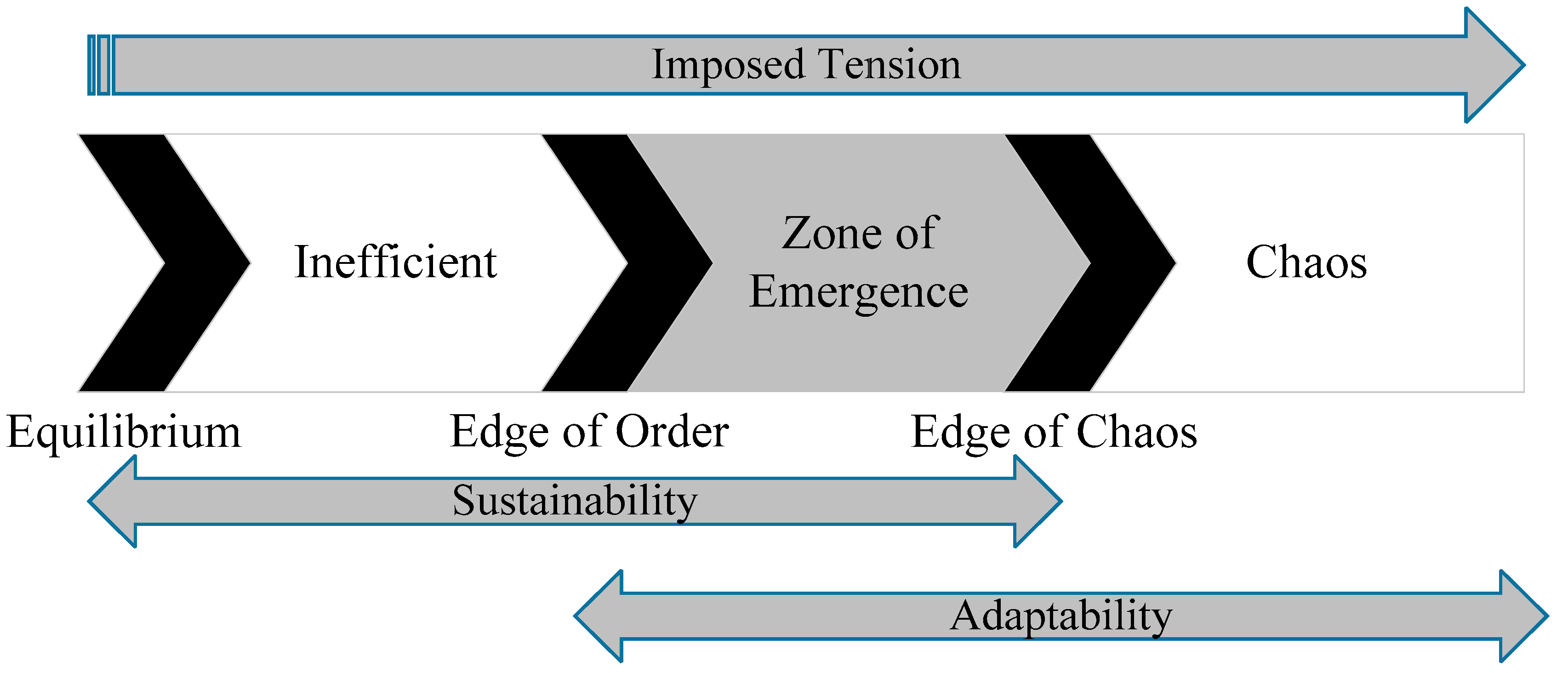
Figure 3.
Schematic representation of the present approach.
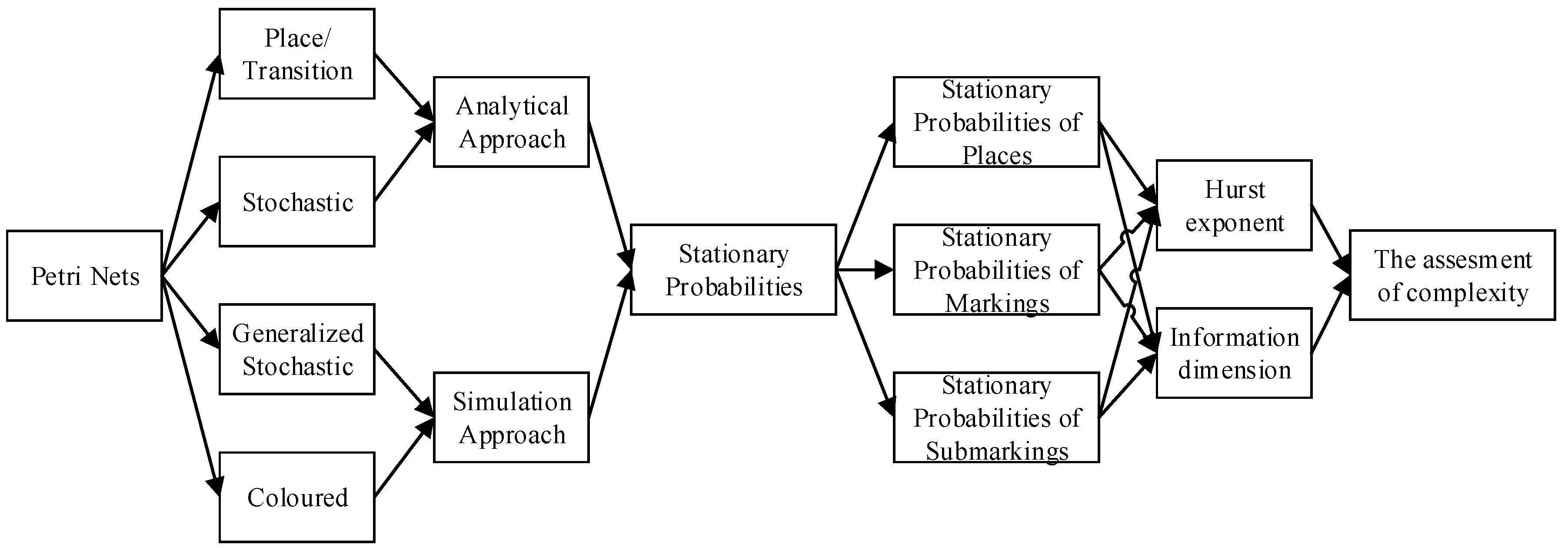
Figure 4.
Simple example.
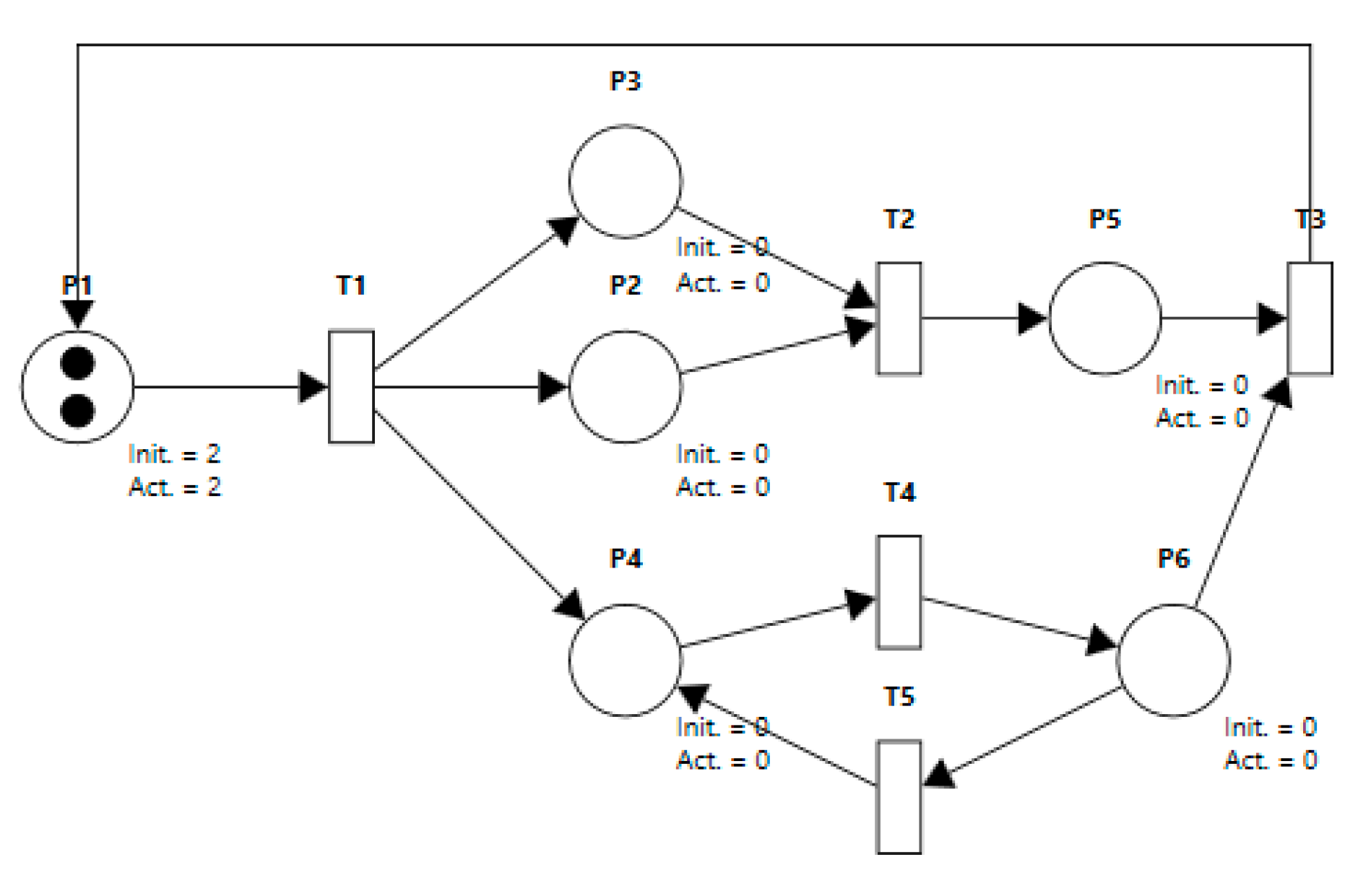
Figure 5.
The development of the fractal dimension (D) depending on the changing constant .

Figure 6.
The development of the generalized Hurst exponent depending on the value of .

Figure 7.
The details of the development of and .
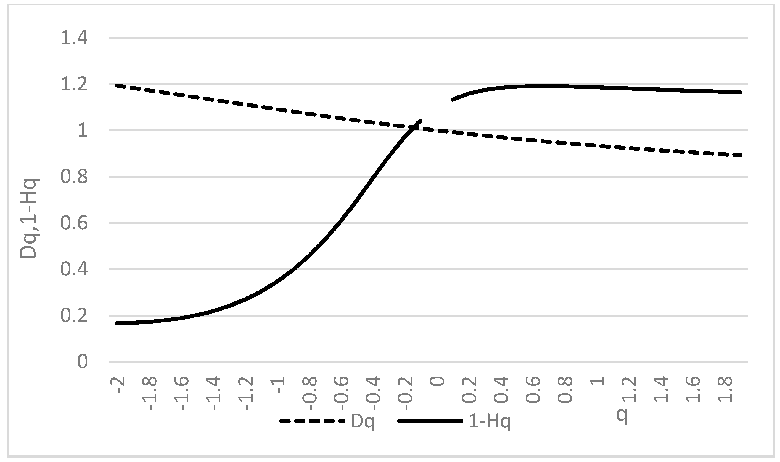
Figure 8.
The development of when changing the number of tokens at .

© 2017 by the authors. Licensee MDPI, Basel, Switzerland. This article is an open access article distributed under the terms and conditions of the Creative Commons Attribution (CC BY) license (http://creativecommons.org/licenses/by/4.0/).
Share and Cite
MDPI and ACS Style
Ibl, M.; Čapek, J. A Behavioural Analysis of Complexity in Socio-Technical Systems under Tension Modelled by Petri Nets. Entropy 2017, 19, 572. https://doi.org/10.3390/e19110572
AMA Style
Ibl M, Čapek J. A Behavioural Analysis of Complexity in Socio-Technical Systems under Tension Modelled by Petri Nets. Entropy. 2017; 19(11):572. https://doi.org/10.3390/e19110572
Chicago/Turabian StyleIbl, Martin, and Jan Čapek. 2017. "A Behavioural Analysis of Complexity in Socio-Technical Systems under Tension Modelled by Petri Nets" Entropy 19, no. 11: 572. https://doi.org/10.3390/e19110572
Note that from the first issue of 2016, this journal uses article numbers instead of page numbers. See further details here.