Minimax Estimation of Quantum States Based on the Latent Information Priors

Abstract

We develop priors for Bayes estimation of quantum states that provide minimax state estimation. The relative entropy from the true density operator to a predictive density operator is adopted as a loss function. The proposed prior maximizes the conditional Holevo mutual information, and it is a quantum version of the latent information prior in classical statistics. For one qubit system, we provide a class of measurements that is optimal from the viewpoint of minimax state estimation.

1. Introduction

In quantum mechanics, the outcome of a measurement is subject to a probability distribution determined from the quantum state of the measured system and the measurement performed. The task of estimating the quantum state from the outcome of measurement is called the quantum estimation and it is a fundamental problem in quantum statistics [1,2,3]. Tanaka and Komaki [4] and Tanaka [5] discussed quantum estimation using the framework of statistical decision theory and showed that Bayesian methods provide better estimation than the maximum likelihood method. In Bayesian methods, we need to specify a prior distribution on the unknown parameters of the quantum states. However, the problem of prior selection has not been fully discussed for quantum estimation [6].

The quantum state estimation problem is related to the predictive density estimation problem in classical statistics [7]. This is a problem of predicting the distribution of an unobserved variable y based on an observed variable x. Suppose $(x,y)\sim p(x,y\mid \theta ),$ where $\theta$ denotes an unknown parameter. Based on the observed x, we predict the distribution $p(y\mid x,\theta )$ of y using a predictive density $\widehat{p}(y\mid x)$. The plug-in predictive density is defined as ${\widehat{p}}_{\mathrm{plug}-\mathrm{in}}(y\mid x)=p(y\mid x,\widehat{\theta }(x))$, where $\widehat{\theta }(x)$ is some estimate of $\theta$ from x. The Bayesian predictive density with respect to a prior distribution $\mathrm{d}\pi (\theta )$ is defined as

$${\widehat{p}}_{\pi }(y\mid x)=\int p(y\mid x,\theta )\mathrm{d}\pi (\theta \mid x)=\frac{\int p(y\mid x,\theta )p(x\mid \theta )\mathrm{d}\pi (\theta )}{\int p(x\mid \theta )\mathrm{d}\pi (\theta )},$$

(1)

where $\mathrm{d}\pi (\theta \mid x)$ is the posterior distribution. We compare predictive densities using the framework of statistical decision theory. Specifically, a loss function $L(q,p)$ is introduced that evaluates the difference between the true density q and the predictive density p. Then, the risk function $R(\theta ,\widehat{p})$ is defined as the average loss when the true value of the parameter is $\theta$:

$$R(\theta ,\widehat{p})=\int L(p(y\mid x,\theta ),\widehat{p}(y\mid x))p(x\mid \theta )\mathrm{d}x.$$

A predictive density ${\widehat{p}}_{\ast }$ is called minimax if it minimizes the maximum risk among all predictive densities:

$$\underset{\theta }{\max }R(\theta ,{\widehat{p}}_{\ast })=\underset{\widehat{p}}{\min }\underset{\theta }{\max }R(\theta ,\widehat{p}).$$

(2)

We adopt the Kullback–Leibler divergence

$$L(q,p)=\int q(x)\log \frac{q(x)}{p(x)}\mathrm{d}x$$

(3)

as a loss function, since it satisfies many desirable properties compared to other loss functions such as the Hellinger distance and the total variation distance [8]. Under this setting, Aitchison [9] proved

$$R(\pi ,{\widehat{p}}_{\pi })=\underset{\widehat{p}}{\min }R(\pi ,\widehat{p}),$$

(4)

where

$$R(\pi ,\widehat{p})=\int R(\theta ,\widehat{p})\pi (\theta )\mathrm{d}\theta$$

is called the Bayes risk. Namely, the Bayesian predictive density ${\widehat{p}}_{\pi }(y\mid x)$ minimizes the Bayes risk. We provide the proof of Equation (4) in the Appendix A. Therefore, it is sufficient to consider only Bayesian predictive densities from the viewpoint of Kullback–Leibler risk, and the selection of the prior $\pi$ becomes important.

For the predictive density estimation problem above, Komaki [10] developed a class of priors called the latent information priors. The latent information prior ${\pi }_{\mathrm{LIP}}$ is defined as a prior that maximizes the conditional mutual information $I_{\theta ,y\mid x}(\pi )$ between the parameter $\theta$ and the unobserved variable y given the observed variable x. Namely,

$$\begin{array}{c}\hfill I_{\theta ,y\mid x}({\pi }_{\mathrm{LIP}})=\underset{\pi }{\max }{I}_{\theta ,y\mid x}(\pi ),\end{array}$$

where

$$\begin{array}{cc}\hfill I_{\theta ,y\mid x}(\pi )& =\int {\sum }_{x,y}p(x,y\mid \theta )\log p(x,y\mid \theta )\mathrm{d}\pi (\theta )-{\sum }_{x,y}{p}_{\pi }(x,y)\log p_{\pi }(x,y)\hfill \\ & -\int {\sum }_{x}p(x\mid \theta )\log p(x\mid \theta )\mathrm{d}\pi (\theta )+{\sum }_x{p}_{\pi }(x)\log p_{\pi }(x)\hfill \end{array}$$

(5)

is the conditional mutual information between y and $\theta$ given x. Here,

$$\begin{array}{c}\hfill p_{\pi }(x,y)=\int p(x,y\mid \theta )\mathrm{d}\pi (\theta ),p_{\pi }(x)=\int p(x\mid \theta )\mathrm{d}\pi (\theta )\end{array}$$

(6)

are marginal densities. The Bayesian predictive densities based on the latent information priors are minimax under the Kullback–Leibler risk:

$$\underset{\theta }{\max }R(\theta ,{\widehat{p}}_{\pi })=\underset{\widehat{p}}{\min }\underset{\theta }{\max }R(\theta ,\widehat{p}).$$

The latent information prior is a generalization of the reference prior [11] that is a prior maximizing the unconditional mutual information $I_{\theta ,y}(\pi )$ between $\theta$ and y.

Now, we consider the problem of estimating the quantum state of a system $\mathrm{Y}$ based on the outcome of a measurement on a system $\mathrm{X}$. Suppose the quantum state of the composed system $(\mathrm{X},\mathrm{Y})$ be ${\sigma }_{\theta }^{\mathrm{X}\mathrm{Y}}$ where $\theta$ denotes an unknown parameter. We perform a measurement on the system $\mathrm{X}$ and obtain the outcome x. Based on the measurement outcome x, we estimate the state of the system $\mathrm{Y}$ by a predictive density operator $\rho (x)$. Similarly to the Bayesian predictive density (1), the Bayesian predictive density operator with respect to the prior $\mathrm{d}\pi (\theta )$ is defined as

$$\begin{array}{c}\hfill {\sigma }_{\pi }^{\mathrm{Y}}(x)=\int {\sigma }_{\theta ,x}^{\mathrm{Y}}\mathrm{d}\pi (\theta \mid x)=\frac{\int {\sigma }_{\theta ,x}^{\mathrm{Y}}p(x\mid \theta )\mathrm{d}\pi (\theta )}{\int p(x\mid \theta )\mathrm{d}\pi (\theta )},\end{array}$$

(7)

where $\mathrm{d}\pi (\theta \mid x)$ is the posterior distribution. Like the predictive density estimation problem discussed above, we compare predictive density operators using the framework of statistical decision theory. There are several possibilities for the loss function $L(\sigma ,\rho )$ in quantum estimation such as the fidelity and the trace norm [12]. In this paper, we adopt the quantum relative entropy

$$L(\sigma ,\rho )=\mathrm{Tr}\sigma (\log \sigma -\log \rho )$$

(8)

as a loss function, since it is a quantum analogue of the Kullback–Leibler divergence (3). Note that the fidelity and the trace norm correspond to the Hellinger distance and the total variation distance in the classical statistics, respectively. Under this setting, Tanaka and Komaki [4] proved that the Bayesian predictive density operators minimize the Bayes risk:

$$\int R(\theta ,{\sigma }_{\pi }^{\mathrm{Y}})\mathrm{d}\pi (\theta )=\underset{\rho }{\min }\int R(\theta ,\rho )\mathrm{d}\pi (\theta ).$$

This is a quantum version of Equation (4).

From Tanaka and Komaki [4], the selection of the prior becomes important also in quantum estimation. However, this problem has not been fully discussed [6]. In this paper, we provide a quantum version of the latent information priors and prove that they provide minimax predictive density operators. Whereas the latent information prior in the classical case maximizes the conditional Shannon mutual information, the proposed prior maximizes the conditional Holevo mutual information. The Holevo mutual information, which is a quantum version of the Shannon mutual information, is a fundamental quantity in the classical-quantum communication [13]. Our result shows that the conditional Holevo mutual information also has a natural meaning in terms of quantum estimation.

Unlike the classical statistics, the measurement is not unique in quantum statistics. Therefore, selection of the measurement also becomes important. From the viewpoint of minimax state estimation, measurements that minimize the minimax risk are considered to be optimal. We provide a class of optimal measurements for one qubit system. This class includes the symmetric informationally complete measurement [14,15]. These measurements and latent information priors provide robust quantum estimation.

2. Preliminaries

2.1. Quantum States and Measurements

We briefly summarize several notations of quantum states and measurements. Let $\mathcal{H}$ be a separable Hilbert space of a quantum system. A Hermitian operator $\rho$ on $\mathcal{H}$ is called a density operator if it satisfies

$$\begin{array}{c}\hfill \mathrm{Tr}\rho =1,\rho \ge 0.\end{array}$$

The state of a quantum system is described by a density operator. We denote the set of all density operators on $\mathcal{H}$ as $\mathcal{S}(\mathcal{H})$.

Denote the set of all linear operators on Hilbert space $\mathcal{H}$ by $\mathcal{L}(\mathcal{H})$ and the set of all positive linear operators by ${\mathcal{L}}_{+}(\mathcal{H})\subset \mathcal{L}(\mathcal{H})$. Let $\Omega$ be a measurable space of all possible outcomes of a measurement and $\mathcal{B}(\Omega )$ be a $\sigma$-algebra of $\Omega$. A map $E:\mathcal{B}(\Omega )\to {\mathcal{L}}_{+}(\mathcal{H})$ is called a positive operator-valued measure (POVM) if it satisfies $E(\varnothing )=O,E(\Omega )=I$, and $E({\cup }_i{B}_i)={\sum }_{i}E(B_i),$ where $B_i\cap B_j=\varnothing ,\forall B_i\in \mathcal{B}(\mathcal{H})$. Any quantum measurement is represented by a POVM on $\Omega$. In this paper, we mainly assume $\Omega$ is finite. In such case, we denote $\Omega =\mathcal{X}=\{1,\cdots ,N\}$ and any POVM is represented by a set of positive Hermitian operators $E=\{E_x\mid x\in \mathcal{X}\}$ such that ${\sum }_{x\in \mathcal{X}}{E}_x=I$.

The outcome of a measurement E on a quantum system with the state $\rho \in \mathcal{S}(\mathcal{H})$ is distributed with a probability measure

$$\begin{array}{c}\hfill \mathrm{Pr}(B)=\mathrm{Tr}E(B)\rho ,B\in \mathcal{B}(\Omega ).\end{array}$$

Let $\mathrm{X}$, $\mathrm{Y}$ be quantum systems with Hilbert spaces ${\mathcal{H}}^{\mathrm{X}}$ and ${\mathcal{H}}^{\mathrm{Y}}$. The Hilbert space of the composed system $(\mathrm{X},\mathrm{Y})$ is given by the tensor product ${\mathcal{H}}^{\mathrm{X}}\otimes {\mathcal{H}}^{\mathrm{Y}}$. Suppose the state of this composed system is ${\sigma }^{\mathrm{X}\mathrm{Y}}$. Then, the states of two subsystems can be yielded by the partial trace:

$$\begin{array}{c}\hfill {\sigma }^{\mathrm{X}}={\mathrm{Tr}}_{\mathrm{Y}}{\sigma }^{\mathrm{X}\mathrm{Y}},{\sigma }^{\mathrm{Y}}={\mathrm{Tr}}_{\mathrm{X}}{\sigma }^{\mathrm{X}\mathrm{Y}}.\end{array}$$

If a measurement $E=\{E_x\mid x\in \mathcal{X}\}$ is performed on the system $\mathrm{X}$ and the measurement outcome is x, then the state of the system $\mathrm{Y}$ becomes

$$\begin{array}{c}\hfill {\sigma }_x^{\mathrm{Y}}=\frac{1}{p_x}{\mathrm{Tr}}_{\mathrm{X}}(E_x\otimes I^{\mathrm{Y}}){\sigma }^{\mathrm{X}\mathrm{Y}},\end{array}$$

where the normalization constant

$$\begin{array}{c}\hfill p_x=\mathrm{Tr}(E_x\otimes I^{\mathrm{Y}}){\sigma }^{\mathrm{X}\mathrm{Y}}\end{array}$$

is the probability of the outcome x. Here, $I^{\mathrm{Y}}$ is the identity operator on the space ${\mathcal{H}}^{\mathrm{Y}}$. We call the operator ${\sigma }_x^{\mathrm{Y}}$ the conditional density operator.

2.2. Quantum State Estimation

We formulate the quantum state estimation problem using the framework of statistical decision theory. Let $\mathrm{X}$ and $\mathrm{Y}$ be quantum systems with finite-dimensional Hilbert spaces ${\mathcal{H}}^{\mathrm{X}}$ and ${\mathcal{H}}^{\mathrm{Y}}$, where $\dim {\mathcal{H}}^{\mathrm{X}}=d_{\mathrm{X}}$ and $\dim {\mathcal{H}}^{\mathrm{Y}}=d_{\mathrm{Y}}$.

Suppose the state of the composed system $(\mathrm{X},\mathrm{Y})$ be ${\sigma }_{\theta }^{\mathrm{X}\mathrm{Y}}$, where $\theta \in \Theta$ denotes unknown parameters. We perform a measurement $E=\{E_x\mid x\in \mathcal{X}\}$ on $\mathrm{X}$, observe the outcome $x\in \mathcal{X}$, and estimate the conditional density operator ${\sigma }_{\theta ,x}^{\mathrm{Y}}$ of $\mathrm{Y}$ by a predictive density operator $\rho (x)$. As discussed in the introduction (1) and (7), the Bayesian predictive density operator based on a prior $\pi (\theta )$ is defined by

$$\begin{array}{c}\hfill {\sigma }_{\pi }^{\mathrm{Y}}(x)=\int {\sigma }_{\theta ,x}^{\mathrm{Y}}\mathrm{d}\pi (\theta \mid x)=\frac{\int {\sigma }_{\theta ,x}^{\mathrm{Y}}p(x\mid \theta )\mathrm{d}\pi (\theta )}{\int p(x\mid \theta )\mathrm{d}\pi (\theta )},\end{array}$$

where $\mathrm{d}\pi (\theta \mid x)$ is the posterior distribution.

To evaluate predictive density operators, we introduce a loss function $L(\sigma ,\rho )$ that evaluates the difference between the true conditional density operator $\sigma$ and the predictive density operator $\rho$. In this paper, we adopt the quantum relative entropy (8) since it is a quantum analogue of the Kullback–Leibler divergence (3). Then, the risk function $R(\theta ,\rho )$ of a predictive density operator $\rho$ is defined by

$$\begin{array}{c}\hfill R(\theta ,\rho )=\sum _{x\in \mathcal{X}}p(x\mid \theta )\mathrm{Tr}{\sigma }_{\theta ,x}^{\mathrm{Y}}(\log {\sigma }_{\theta ,x}^{\mathrm{Y}}-\log \rho (x)),\end{array}$$

where

$$\begin{array}{c}\hfill p(x\mid \theta )=\mathrm{Tr}(E_x\otimes I^{\mathrm{Y}}){\sigma }_{\theta }^{\mathrm{X}\mathrm{Y}}=\mathrm{Tr}{E}_x{\sigma }_{\theta }^{\mathrm{X}}\end{array}$$

is the probability of the outcome x. Similarly to the classical case (2), a predictive density operator ${\rho }_{\ast }$ is called minimax if it minimizes the maximum risk among all predictive density operators [16,17]:

$$\underset{\theta }{\max }R(\theta ,{\rho }_{\ast })=\underset{\rho }{\min }\underset{\theta }{\max }R(\theta ,\rho ).$$

Tanaka and Komaki [4] showed

$$\begin{array}{c}\hfill R(\pi ,{\sigma }_{\pi }^{\mathrm{Y}})=\underset{\rho }{\min }R(\pi ,\rho ),\end{array}$$

(9)

where

$$\begin{array}{c}\hfill R(\pi ,\rho )=\int R(\theta ,\rho )\mathrm{d}\pi (\theta )\end{array}$$

is called the Bayes risk. Namely, the Bayesian predictive density operator minimizes the Bayes risk. This result is a quantum version of Equation (4). Although Tanaka and Komaki [4] considered separable models (${\sigma }_{\theta }^{\mathrm{X}\mathrm{Y}}={\sigma }_{\theta }^{\mathrm{X}}\otimes {\sigma }_{\theta }^{\mathrm{Y}}$), the relation (9) holds also for non-separable models as shown in the Appendix A. Therefore, it is sufficient to consider only Bayesian predictive density operators and the problem of prior selection becomes crucial.

2.3. Notations

For a quantum state family $\{{\sigma }_{\theta }^{\mathrm{X}\mathrm{Y}}\mid \theta \in \Theta \}$, we define another quantum state family

$$\mathcal{M}=\{{\oplus }_{x}p(x\mid \theta ){\sigma }_{\theta ,x}^{\mathrm{Y}}\mid \theta \in \Theta \},$$

where

$$\begin{array}{c}\hfill {\oplus }_{x}p(x\mid \theta ){\sigma }_{\theta ,x}^{\mathrm{Y}}=\left(\begin{array}{cccc}p(1\mid \theta ){\sigma }_{\theta ,1}^{\mathrm{Y}}& O& \cdots & O\\ O& p(2\mid \theta ){\sigma }_{\theta ,2}^{\mathrm{Y}}& & ⋮\\ ⋮& & \ddots & O\\ O& \cdots & O& p(N\mid \theta ){\sigma }_{\theta ,N}^{\mathrm{Y}}\end{array}\right)\end{array}$$

is a density operator in ${\mathbb{C}}^N\otimes {\mathcal{H}}^{\mathrm{Y}}$. Since $\dim {\mathbb{C}}^N\otimes {\mathcal{H}}^{\mathrm{Y}}=N{d}_{\mathrm{Y}}$, the state family $\mathcal{M}$ can be regarded as a subset of the Euclidean space ${\mathbb{R}}^{N^2{d}_{\mathrm{Y}}^2-1}$. By identifying $\Theta$ with $\mathcal{M}$, the parameter space $\Theta$ is endowed with the induced topology as a subset of ${\mathbb{R}}^{N{d}_{\mathrm{Y}}^2-1}$.

Any measurement on the system $\mathrm{X}$ is represented by a projective measurement $\{e_{xx}=|x\rangle \langle x|\mid x=1,\cdots ,N\}$, where $\{|1\rangle ,\cdots ,|N\rangle \}$ is an orthonormal basis of ${\mathbb{C}}^N$. For every $x\in \mathcal{X}$, we define $S_{\theta }(x)\in {\mathcal{L}}_{+}({\mathcal{H}}^{\mathrm{Y}})$ as

$$\begin{array}{cc}\hfill S_{\theta }(x):=& {\mathrm{Tr}}_{{\mathbb{C}}^N}(e_{xx}\otimes I^{\mathrm{Y}})({\oplus }_{x}p(x\mid \theta ){\sigma }_{\theta ,x}^{\mathrm{Y}})=p(x\mid \theta ){\sigma }_{\theta ,x},\hfill \end{array}$$

which is the unnormalized state of $\mathrm{Y}$ conditional on the measurement outcome x. We also define

$$\begin{array}{c}\hfill S_{\pi }(x)=\int S_{\theta }(x)\mathrm{d}\pi (\theta ),p_{\pi }(x)=\mathrm{Tr}{S}_{\pi }(x),{\sigma }_{\pi }(x)=\frac{S_{\pi }(x)}{p_{\pi }(x)}.\end{array}$$

3. Minimax Estimation of Quantum States

In this section, we develop the latent information prior for quantum state estimation and show that this prior provides a minimax predictive density operator.

In the following, we assume the following conditions:

• $\Theta$ is compact.
• For every $x\in \mathcal{X}$, $E_x\ne O$.
• For every $x\in \mathcal{X}$, there exists $\theta \in \Theta$ such that $p(x\mid \theta )=\mathrm{Tr}{E}_x{\sigma }_{\theta }^{\mathrm{X}}>0$.

The third assumption is achieved by adopting sufficiently small Hilbert space. Namely, if there exists $x\in \mathcal{X}$ such that $p(x\mid \theta )=\mathrm{Tr}{E}_x{\sigma }_{\theta }^{\mathrm{X}}=0$ for every $\theta \in \Theta$, then we redefine the state space $\mathcal{H}$ as the orthogonal complement of $\mathrm{Ker}{E}_x$.

Let $\mathcal{P}$ be the set of all probability measures on $\Theta$ endowed with the weak convergence topology and the corresponding Borel algebra. By the Prohorov theorem [18] and the first assumption, $\mathcal{P}$ is compact.

When x is fixed, the function $\theta \in \Theta \mapsto S_{\theta }(x)$ is bounded and continuous. Thus, for every fixed $x\in \mathcal{X}$, the function

$$\begin{array}{c}\hfill \pi \in \mathcal{P}\mapsto S_{\pi }(x)=\int S_{\theta }(x)\mathrm{d}\pi (\theta )\end{array}$$

is continuous because $\mathcal{P}$ is endowed with the weak convergence topology and $\dim {\mathcal{H}}^{\mathrm{Y}}<\infty$. Let ${\{{\lambda }_{x,i}\}}_i,\{|{\varphi }_{x,i}\rangle {\}}_i$ be the eigenvalues and the normalized eigenvectors of the predictive density operator $\rho (x)$. For every predictive density operator $\rho$, consider the function from $\mathcal{P}$ to $[0,\infty ]$ defined by

$$\begin{array}{cc}\hfill D_{\rho }(\pi )& =\sum _x\mathrm{Tr}{S}_{\pi }(x)(\log S_{\pi }(x)-\log (p_{\pi }(x)\rho (x)))\hfill \\ & =\sum _x\mathrm{Tr}{S}_{\pi }(x)(\log S_{\pi }(x)-(\log p_{\pi }(x))I-\log \rho (x))\hfill \\ & =\sum _x\mathrm{Tr}{S}_{\pi }(x)\log S_{\pi }(x)-\sum _x{p}_{\pi }(x)\log p_{\pi }(x)\hfill \\ & \hspace{1em}+\sum _{i:{\lambda }_{x,i}\ne 0}-p_{\pi }(x)\langle {\varphi }_{x,i}|{\sigma }_{\pi }(x)|{\varphi }_{x,i}\rangle \log {\lambda }_{x,i}\hfill \\ & \hspace{1em}+\sum _{i:{\lambda }_{x,i}=0}-p_{\pi }(x)\langle {\varphi }_{x,i}|{\sigma }_{\pi }(x)|{\varphi }_{x,i}\rangle \log {\lambda }_{x,i}.\hfill \end{array}$$

(10)

The last term in (10) is lower semicontinuous under the definition $0\log 0=0$ [10], since each summand takes either zero or infinity and so the set of $\pi \in \mathcal{P}$ such that this term takes zero is closed. In addition, the other terms in (10) are continuous since the von Neumann entropy is continuous [12]. Therefore, the function $D_{\rho }(\pi )$ in (10) is lower-semicontinuous.

Now, we prove that the class of predictive density operators that are limits of Bayesian predictive density operators is an essentially complete class. We prepare three lemmas. Lemma 1 is useful for differentiation of quantum relative entropy (see Hiai and Petz [19]). Lemmas 2 and 3 are from Komaki [10].

Lemma 1.

Let $A,B$ be n-dimensional self-adjoint matrices and t be a real number. Assume that $f:(\alpha ,\beta )\to \mathbb{R}$ is a continuously differentiable function defined on an interval and assume that the eigenvalues of $A+tB$ are in $(\alpha ,\beta )$ if t is sufficiently close to $t_0$. Then,

$$\begin{array}{c}\hfill \frac{\mathrm{d}}{\mathrm{d}t}\mathrm{Tr}f(A+tB){|}_{t=t_0}=\mathrm{Tr}(B{f}^{\prime }(A+t_{0}B)).\end{array}$$

Lemma 2

([10]). Let μ be a probability measure on Θ. Then,

$${\mathcal{P}}_{\epsilon \mu }=\{\epsilon \mu +(1-\epsilon )\pi \mid \pi \in \mathcal{P}\}$$

is a closed subset of $\mathcal{P}$ for $0\le \epsilon \le 1$.

Lemma 3

([10]). Let $f:\mathcal{P}\to [0,\infty ]$ be continuous, and let μ be a probability measure on Θ such that $p_{\mu }(x):=\int p(x\mid \theta )d\mu (\theta )>0$ for every $x\in \mathcal{X}$. Then, there is a probability measure ${\pi }_n$ in

$$\begin{array}{c}\hfill {\mathcal{P}}_{\mu /n}=\left\{\frac{1}{n}\mu +\left(1-\frac{1}{n}\right)\pi \mid \pi \in \mathcal{P}\right\}\end{array}$$

for every n, such that $f({\pi }_n)={\inf }_{\pi \in {\mathcal{P}}_{\mu /n}}f(\pi )$. Furthermore, there exists a convergent subsequence ${\{{\pi }_m^{\prime }\}}_{m=1}^{\infty }$ of ${\{{\pi }_n\}}_{n=1}^{\infty }$ and the equality $f({\pi }_{\infty }^{\prime })={\inf }_{\pi \in \mathcal{P}}f(\pi )$ holds, where ${\pi }_{\infty }^{\prime }={\lim }_{m\to \infty }{\pi }_m^{\prime }$.

By using these results, we obtain the following theorem, which is a quantum version of Theorem 1 of Komaki [10].

Theorem 1.

(1) 

Let $\rho (x)$ be a predictive density operator. If there exists a prior ${\widehat{\pi }}^{\rho }\in \mathcal{P}$ such that $D_{\rho }({\widehat{\pi }}^{\rho })={\inf }_{\pi \in \mathcal{P}}{D}_{\rho }(\pi )$ and $p_{{\widehat{\pi }}^{\rho }}(x)>0$ for every $x\in \mathcal{X}$, then $R(\theta ,{\sigma }_{{\widehat{\pi }}^{\rho }}(x))\le R(\theta ,\rho (x))$ for every $\theta \in \Theta$.

(2) 

For every predictive density operator ρ, there exists a convergent prior sequence ${\{{\pi }_n^{\rho }\}}_{n=1}^{\infty }$ such that $D_{\rho }({\lim }_{n\to \infty }{\pi }_n^{\rho })={\inf }_{\pi \in \mathcal{P}}{D}_{\rho }(\pi )$, ${\lim }_{n\to \infty }{\sigma }_{{\pi }_n^{\rho }}(x)$ exists, and $R(\theta ,{\lim }_{n\to \infty }{\sigma }_{{\pi }_n^{\rho }}(x))\le R(\theta ,\rho )$ for every $\theta \in \Theta$.

Next, we develop priors that provide minimax predictive density operators. Let x be a random variable, which represents the outcome of the measurement, i.e., $x\sim p(·\mid \theta )$. Then, as a quantum analogue of the conditional mutual information (5), we define the conditional Holevo mutual information [13] between the quantum state ${\sigma }_x^Y$ of Y and the parameter $\theta$ given the measurement outcome x as

$$\begin{array}{cc}\hfill I_{\theta ,\sigma \mid x}(\pi )& =\int {\sum }_x\mathrm{Tr}{S}_{\theta }(x)\log S_{\theta }(x)\mathrm{d}\pi (\theta )-{\sum }_x\mathrm{Tr}{S}_{\pi }(x)\log S_{\pi }(x)\hfill \\ & -\int {\sum }_{x}p(x\mid \theta )\log p(x\mid \theta )\mathrm{d}\pi (\theta )+{\sum }_x{p}_{\pi }(x)\log p_{\pi }(x)\hfill \\ & =\int {\sum }_{x}p(x\mid \theta )\mathrm{Tr}{\sigma }_{\theta ,x}(\log {\sigma }_{\theta ,x}-\log {\sigma }_{\pi ,x})\mathrm{d}\pi (\theta ),\hfill \end{array}$$

(11)

which is a function of $\pi \in \mathcal{P}$. Here, we used

$$\begin{array}{cc}\hfill \sum _x\mathrm{Tr}{S}_{\theta }(x)\log S_{\theta }(x)& =\sum _{x}p(x\mid \theta )\mathrm{Tr}{\sigma }_{\theta ,x}(\log p(x\mid \theta )I+\log {\sigma }_{\theta ,x})\hfill \\ & =\sum _{x}p(x\mid \theta )\log p(x\mid \theta )+\sum _{x}p(x\mid \theta )\mathrm{Tr}{\sigma }_{\theta ,x}\log {\sigma }_{\theta ,x}\hfill \end{array}$$

and

$$\begin{array}{cc}\hfill \sum _x\mathrm{Tr}{S}_{\pi }(x)\log S_{\pi }(x)& =\sum _x{p}_{\pi }(x)\mathrm{Tr}{\sigma }_{\pi }(x)(\log p_{\pi }(x)I+\log {\sigma }_{\pi }(x))\hfill \\ & =\sum _x{p}_{\pi }(x)\log p_{\pi }(x)+\sum _x{p}_{\pi }(x)\mathrm{Tr}{\sigma }_{\pi }(x)\log {\sigma }_{\pi }(x).\hfill \end{array}$$

The conditional Holevo mutual information provides an upper bound on the conditional mutual information as follows.

Proposition 1.

Let ${\sigma }_{\theta }^{XY}$ be the state of the composed system $(X,Y)$. Suppose that a measurement is performed on X with the measurement outcome x and then another measurement is performed on Y with the measurement outcome y. Then,

$$\begin{array}{c}\hfill I_{\theta ,\sigma \mid x}(\pi )\ge I_{\theta ,y\mid x}(\pi ).\end{array}$$

(12)

Proof. 

Since any measurement is a trace-preserving completely positive map, inequality (12) follows from the monotonicity of the quantum relative entropy [13]. ☐

Analogous with the latent information priors [10] in classical statistics, we define latent information priors as priors that maximize the conditional Holevo mutual information. It is expected that the Bayesian predictive density operator ${\sigma }_{\widehat{\pi },x}$ based on a latent information prior is a minimax predictive density operator. This is true from the following theorem, which is a quantum version of Theorem 2 of Komaki [10].

Theorem 2.

(1) 

Let $\widehat{\pi }\in \mathcal{P}$ be a prior maximizing $I_{\theta ,\sigma \mid x}(\pi )$. If $p_{\widehat{\pi }}(x)>0$ for all $x\in \mathcal{X}$; then, ${\sigma }_{\widehat{\pi }}(x)$ is a minimax predictive density operator.

(2) 

There exists a convergent prior sequence ${\{{\pi }_n\}}_{n=1}^{\infty }$ such that ${\lim }_{n\to \infty }{\sigma }_{{\pi }_n}(x)$ is a minimax predictive density operator and the equality $I_{\theta ,\sigma \mid x}({\pi }_{\infty })={\sup }_{\pi \in \mathcal{P}}{I}_{\theta ,\sigma \mid x}(\pi )$ holds.

The proof of Theorems 1 and 2 are deferred to the Appendix A.

We note that the minimax risk ${\inf }_{\rho }{\sup }_{\theta }{R}_E(\theta ,\rho )$ depends on the measurement E on $\mathrm{X}$. Therefore, the measurement E with minimum minimax risk is desirable from the viewpoint of minimaxity. We define a POVM $E^{\ast }$ to be a minimax POVM if it satisfies

$$\underset{\rho }{\inf }\underset{\theta }{\sup }{R}_{E^{\ast }}(\theta ,\rho )=\underset{E}{\inf }\underset{\rho }{\inf }\underset{\theta }{\sup }{R}_E(\theta ,\rho ).$$

(13)

In the next section, we provide a class of minimax POVMs for one qubit system.

4. One Qubit System

In this section, we consider one qubit system and derive a class of minimax POVMs satisfying (13).

Qubit is a quantum system with a two-dimensional Hilbert space. It is the fundamental system in the quantum information theory. A general state of one qubit system is described by a density matrix

$$\begin{array}{c}\hfill {\sigma }_{\theta }=\frac{1}{2}\left(\begin{array}{cc}1+{\theta }_z& {\theta }_x-i{\theta }_y\\ {\theta }_x+i{\theta }_y& 1-{\theta }_z\end{array}\right),\end{array}$$

where $\theta ={({\theta }_x,{\theta }_y,{\theta }_z)}^{\top }\in \Theta =\{{({\theta }_x,{\theta }_y,{\theta }_z)}^{\top }\in {\mathbb{R}}^3\mid {\parallel \theta \parallel }^2\le 1\}$. The parameter space $\partial \Theta =\{{({\theta }_x,{\theta }_y,{\theta }_z)}^{\top }\in {\mathbb{R}}^3\mid \parallel \theta {\parallel }^2=1\}$ for pure states is called the Bloch sphere.

Let ${\sigma }_{\theta }^{XY}={\sigma }_{\theta }\otimes {\sigma }_{\theta }$ be a separable state. We consider the estimation of ${\sigma }_{\theta }^Y={\sigma }_{\theta }$ from the outcome of a measurement on ${\sigma }_{\theta }^X={\sigma }_{\theta }$. Here, we assume that the state ${\sigma }_{\theta }^{XY}$ is separable, since the state of Y changes according to the outcome of the measurement on X and so the estimation problem is not well-defined if the state ${\sigma }_{\theta }^{XY}$ is not separable.

Let $\Omega :=\{{(x,y,z)}^{\top }\in {\mathbb{R}}^3\mid x^2+y^2+z^2=1\}$ and $\mathcal{B}=\mathcal{B}(\Omega )$ be Borel sets. From Haapasalo et al. [20], it is sufficient to consider POVMs on $\Omega$. For every probability measure $\mu$ on $(\Omega ,\mathcal{B})$ that satisfies

$${\int }_{\Omega }xd\mu (\omega )={\int }_{\Omega }yd\mu (\omega )={\int }_{\Omega }zd\mu (\omega )=0,$$

we define a POVM $E:\mathcal{B}\to {\mathcal{L}}_{+}$ by

$$E(B)={\int }_B\left(\begin{array}{cc}1+z& x-iy\\ x+iy& 1-z\end{array}\right)\mathrm{d}\mu (\omega ).$$

In the following, we identify E with $\mu$.

Let ${\mathcal{E}}_{1-\mathrm{qubit}}^{\ast }$ be a class of POVMs on $\Omega$ represented by measures that satisfy the conditions

$$\begin{array}{c}{E}_{\mu }[x]=E_{\mu }[y]=E_{\mu }[z]=0,\hfill \\ E_{\mu }[xy]=E_{\mu }[yz]=E_{\mu }[zx]=0,\hfill \\ E_{\mu }[x^2]=E_{\mu }[y^2]=E_{\mu }[z^2]=\frac{1}{3},\hfill \end{array}$$

where $E_{\mu }$ is the expectation with respect to a measure $\mu$. We provide two examples of POVMs in ${\mathcal{E}}_{1-\mathrm{qubit}}^{\ast }$.

Proposition 2.

The POVM corresponding to

$$\begin{array}{c}\hfill \mu (\mathrm{d}\omega )=\frac{1}{4\pi }\mathrm{d}\omega ,\end{array}$$

(14)

where $d\omega$ is surface element, is in ${\mathcal{E}}_{1-\mathrm{qubit}}^{\ast }$.

Proof. 

From the symmetry of $\mu$, $E_{\mu }[x]=E_{\mu }[y]=E_{\mu }[z]=E_{\mu }[xy]=E_{\mu }[yz]=E_{\mu }[zx]=0$. Moreover, from $E_{\mu }[1]=E_{\mu }[x^2+y^2+z^2]=1$ and the symmetry of $\mu$, $E_{\mu }[x^2]=E_{\mu }[y^2]=E_{\mu }[z^2]=1/3$. ☐

Proposition 3.

Suppose that ${\omega }_i(i=1,2,3,4)\in \Omega$ satisfies $|{\omega }_i{|}^2=1,{\omega }_i·{\omega }_j=-1/3(i\ne j)$. Let μ be a four point discrete measure on Ω defined by

$$\begin{array}{c}\hfill \mu (\{{\omega }_1\})=\mu (\{{\omega }_2\})=\mu (\{{\omega }_3\})=\mu (\{{\omega }_4\})=\frac{1}{4}.\end{array}$$

(15)

Then, the POVM corresponding to μ belongs to ${\mathcal{E}}_{1-\mathrm{qubit}}^{\ast }$.

Proof. 

Let $P=({\omega }_1,{\omega }_2,{\omega }_3,{\omega }_4)\in {\mathbb{R}}^{3\times 4}$ and $\mathbf{1}={(1,1,1,1)}^{\top }$. From the assumption on ${\omega }_i(i=1,2,3,4)$,

$$P^{\top }P=\frac{4}{3}{I}_4-\frac{1}{3}{J}_4,$$

(16)

where $I_4\in {\mathbb{R}}^{4\times 4}$ is the identity matrix and $J_4=\mathbf{1}{\mathbf{1}}^{\top }\in {\mathbb{R}}^{4\times 4}$ is a matrix whose elements are all one. From (16), we have ${\mathbf{1}}^{\top }{P}^{\top }P\mathbf{1}={\parallel P\mathbf{1}\parallel }^2=0$. Therefore, $P\mathbf{1}=0$ and it implies $E_{\mu }[x]=E_{\mu }[y]=E_{\mu }[z]=0$.

In addition, from (16),

$$\begin{array}{cc}\hfill P^{\top }P{P}^{\top }P& =((4/3)I_4-(1/3)J_4)((4/3)I_4-(1/3)J_4)\hfill \\ & =(4/3)((4/3)I_4-(1/3)J_4)\hfill \\ & =(4/3)P^{\top }P.\hfill \end{array}$$

Therefore, $P^{\top }(P{P}^{\top }-(4/3)I_3)P=0$. Since $\mathrm{rank}P=3$, it implies $P{P}^{\top }=(4/3)I_3$. Then, $E_{\mu }[xy]=E_{\mu }[yz]=E_{\mu }[zx]=0$ and $E_{\mu }[x^2]=E_{\mu }[y^2]=E_{\mu }[z^2]=1/3$. ☐

We note that the POVM (15) is a special case of the SIC-POVM (symmetric, informationally complete, positive operator valued measure) [14,15].

Let ${\mathcal{P}}_{1-\mathrm{qubit}}^{\ast }$ be a class of priors on $\Theta$ that satisfies the conditions

$$\begin{array}{c}{E}_{\pi }[{\theta }_x]=E_{\pi }[{\theta }_y]=E_{\pi }[{\theta }_z]=0,\hfill \\ E_{\pi }[{\theta }_x{\theta }_y]=E_{\pi }[{\theta }_y{\theta }_z]=E_{\pi }[{\theta }_z{\theta }_x]=0,\hfill \\ E_{\pi }[{\theta }_x^2]=E_{\pi }[{\theta }_y^2]=E_{\pi }[{\theta }_z^2]=\frac{1}{3},\hfill \end{array}$$

where $E_{\pi }$ is the expectation with respect to a prior $\pi$.

Proposition 4.

The uniform prior

$$\begin{array}{c}\hfill \pi (\mathrm{d}\theta )=\frac{1}{4\pi }\mathrm{d}\theta ,\end{array}$$

where $\mathrm{d}\theta$ is the surface element on the Bloch sphere, belongs to ${\mathcal{P}}_{1-\mathrm{qubit}}^{\ast }$.

Proof. 

Same as Proposition 2. ☐

Proposition 5.

Suppose that ${\theta }_i(i=1,2,3,4)\in \Theta$ satisfies $|{\theta }_i{|}^2=1,{\theta }_i·{\theta }_j=-1/3(i\ne j)$. Then, the four point discrete prior

$$\begin{array}{c}\hfill \pi (\{{\theta }_1\})=\pi (\{{\theta }_2\})=\pi (\{{\theta }_3\})=\pi (\{{\theta }_4\})=\frac{1}{4}\end{array}$$

belongs to ${\mathcal{P}}_{1-\mathrm{qubit}}^{\ast }$.

Proof. 

Same as Proposition 3. ☐

We obtain the following result.

Lemma 4.

Suppose ${\pi }^{\ast }\in {\mathcal{P}}_{1-\mathrm{qubit}}^{\ast }$. Then, for general measurement E, the risk function of the Bayesian predictive density operator ${\sigma }_{{\pi }^{\ast }}$ is

$$\begin{array}{cc}\hfill R_E(\theta ,{\sigma }_{{\pi }^{\ast }})=-& h\left(\frac{1+\parallel \theta \parallel }{2}\right)+\frac{1}{2}\log \frac{9}{2}-\frac{\log 2}{2}({{\theta }_x}^2{E}_{\mu }[x^2]+{{\theta }_y}^2{E}_{\mu }[y^2]+{{\theta }_z}^2{E}_{\mu }[z^2]\hfill \\ & +2{\theta }_x{\theta }_y{E}_{\mu }[xy]+2{\theta }_y{\theta }_z{E}_{\mu }[yz]+2{\theta }_z{\theta }_x{E}_{\mu }[zx]).\hfill \end{array}$$

Proof. 

The distribution of the measurement outcome $\omega ={(x,y,z)}^{\top }$ is

$$\begin{array}{cc}\hfill p(B\mid \theta )& =\mathrm{Tr}{\sigma }_{\theta }E(B)=(1+x{\theta }_x+y{\theta }_y+z{\theta }_z)\mu (B).\hfill \end{array}$$

Then, since ${\pi }^{\ast }\in {\mathcal{P}}_{1-\mathrm{qubit}}^{\ast }$, the marginal distribution of the measurement outcome is

$$\begin{array}{cc}\hfill p(B)& ={\int }_{\Theta }p(B\mid \theta )\mathrm{d}{\pi }^{\ast }(\theta )={\int }_{\Theta }(1+x{\theta }_x+y{\theta }_y+z{\theta }_z)\mu (B)\mathrm{d}{\pi }^{\ast }(\theta )=\mu (B).\hfill \end{array}$$

Therefore, the posterior distribution of $\theta$ is

$$\begin{array}{cc}\hfill \mathrm{d}{\pi }^{\ast }(\theta \mid \omega )& =(1+x{\theta }_x+y{\theta }_y+z{\theta }_z)\mathrm{d}{\pi }^{\ast }(\theta ).\hfill \end{array}$$

The posterior mean of ${\theta }_x,{\theta }_y$ and ${\theta }_z$ are $x/3,y/3$ and $z/3$, respectively.

Thus, the Bayesian predictive density operator based on prior ${\pi }^{\ast }$ is

$$\begin{array}{cc}\hfill {\sigma }_{{\pi }^{\ast }}(\omega )& =\int {\sigma }_{\theta }\mathrm{d}{\pi }^{\ast }(\theta \mid \omega )=\frac{1}{2}\left(\begin{array}{cc}1+z/3& x/3-iy/3\\ x/3+iy/3& 1-z/3\end{array}\right),\hfill \end{array}$$

and we have

$$\begin{array}{c}\hfill \log {\sigma }_{{\pi }^{\ast }}(\omega )=\left(\begin{array}{cc}(\log {\displaystyle \frac{1}{3}})({\displaystyle \frac{1-z}{2}})& (\log {\displaystyle \frac{1}{3}})({\displaystyle \frac{-x+iy}{2}})\\ (\log {\displaystyle \frac{1}{3}})({\displaystyle \frac{-x-iy}{2}})& (\log {\displaystyle \frac{1}{3}})({\displaystyle \frac{1+z}{2}})\end{array}\right)+\left(\begin{array}{cc}(\log {\displaystyle \frac{2}{3}})({\displaystyle \frac{1+z}{2}})& (\log {\displaystyle \frac{2}{3}})(\frac{x-iy}{2})\\ (\log {\displaystyle \frac{2}{3}})({\displaystyle \frac{x+iy}{2}})& (\log {\displaystyle \frac{2}{3}})(\frac{1-z}{2})\end{array}\right).\end{array}$$

Therefore, the quantum relative entropy loss is

$$\begin{array}{cc}\hfill D({\sigma }_{\theta },{\sigma }_{{\pi }^{\ast }}(\omega ))& =\mathrm{Tr}{\sigma }_{\theta }(\log {\sigma }_{\theta }-\log {\sigma }_{{\pi }^{\ast }}(\omega ))\hfill \\ & =-h\left(\frac{1+\parallel \theta \parallel }{2}\right)+\frac{1}{2}\log \frac{9}{2}-\frac{x{\theta }_x+y{\theta }_y+z{\theta }_z}{2}\log 2.\hfill \end{array}$$

Hence, the risk function is

$$\begin{array}{cc}\hfill R_E(\theta ,{\sigma }_{{\pi }^{\ast }})& ={\int }_{\Omega }D({\sigma }_{\theta },{\sigma }_{{\pi }^{\ast }}(\omega ))\mathrm{d}p(\omega \mid \theta )\hfill \\ & =-h\left(\frac{1+\parallel \theta \parallel }{2}\right)+\frac{1}{2}\log \frac{9}{2}-\frac{\log 2}{2}({{\theta }_x}^2{E}_{\mu }[x^2]+{{\theta }_y}^2{E}_{\mu }[y^2]+{{\theta }_z}^2{E}_{\mu }[z^2]\hfill \\ & +2{\theta }_x{\theta }_y{E}_{\mu }[xy]+2{\theta }_y{\theta }_z{E}_{\mu }[yz]+2{\theta }_z{\theta }_x{E}_{\mu }[zx]).\hfill \end{array}$$

 ☐

Theorem 3.

For a measurement $E\in {\mathcal{E}}_{1-\mathrm{qubit}}^{\ast }$, every ${\pi }^{\ast }\in {\mathcal{P}}_{1-\mathrm{qubit}}^{\ast }$ is a latent information prior:

$$\begin{array}{c}\hfill \underset{\theta }{\max }R(\theta ,{\sigma }_{{\pi }^{\ast }})=\underset{\rho }{\min }\underset{\theta }{\max }R(\theta ,\rho ).\end{array}$$

In addition, the risk of the Bayesian predictive density operator based on ${\pi }^{\ast }$ is

$$\begin{array}{c}\hfill R(\theta ,{\sigma }_{{\pi }^{\ast }})=-h\left(\frac{1+\parallel \theta \parallel }{2}\right)+\frac{1}{2}\log \frac{9}{2}-\frac{\log 2}{6}{\parallel \theta \parallel }^2,\end{array}$$

where h is the binary entropy function $h(p)=-p\log p-(1-p)\log (1-p)$.

Proof. 

From Lemma 4 and $E^{\ast }\in {\mathcal{E}}_{1-\mathrm{qubit}}^{\ast }$,

$$\begin{array}{c}\hfill R_{E^{\ast }}(\theta ,{\sigma }_{{\pi }^{\ast }})=-h\left(\frac{1+\left|\theta \right|}{2}\right)+\frac{1}{2}\log \frac{9}{2}-\frac{\log 2}{6}({{\theta }_x}^2+{{\theta }_y}^2+{{\theta }_z}^2).\end{array}$$

Therefore, the risk depends only on $r=\parallel \theta \parallel$ and we have

$$\begin{array}{c}\hfill R_{E^{\ast }}(\theta ,{\sigma }_{{\pi }^{\ast }})=g(r)=-h\left(\frac{1+r}{2}\right)+\frac{1}{2}\log \frac{9}{2}-\frac{\log 2}{6}{r}^2.\end{array}$$

(17)

Since

$$\begin{array}{cc}\hfill g^{\prime }(r)=& \frac{1}{2}\log \left(\frac{1+r}{1-r}\right)-\frac{\log 2}{3}r,\hfill \end{array}$$

$$\begin{array}{cc}\hfill g^{″}(r)=& \frac{1}{1-r^2}-\frac{\log 2}{3}\ge 1-\frac{\log 2}{3}\ge 0,\hfill \end{array}$$

the function $g(r)$ is convex. In addition, we have $g(1)=\log 3-\frac{2}{3}\log 2>g(0)=\log 3-\frac{3}{2}\log 2$. Therefore, $g(r)$ takes the maximum at $r=1$.

In other words, $R_{E^{\ast }}(\theta ,{\sigma }_{{\pi }^{\ast }})$ takes maximum on the Bloch sphere. In addition, since $\int ({\theta }_x^2+{\theta }_y^2+{\theta }_z^2)\mathrm{d}{\pi }^{\ast }(\theta )=1/3+1/3+1/3=1$, the support of ${\pi }^{\ast }$ is included in the Bloch sphere ${\parallel \theta \parallel }^2=1$. Therefore, $\int R_{E^{\ast }}(\theta ,{\sigma }_{{\pi }^{\ast }})\mathrm{d}{\pi }^{\ast }(\theta )={\sup }_{\theta }{R}_{E^{\ast }}(\theta ,{\sigma }_{{\pi }^{\ast }})$ and it implies that ${\pi }^{\ast }$ is a latent information prior. ☐

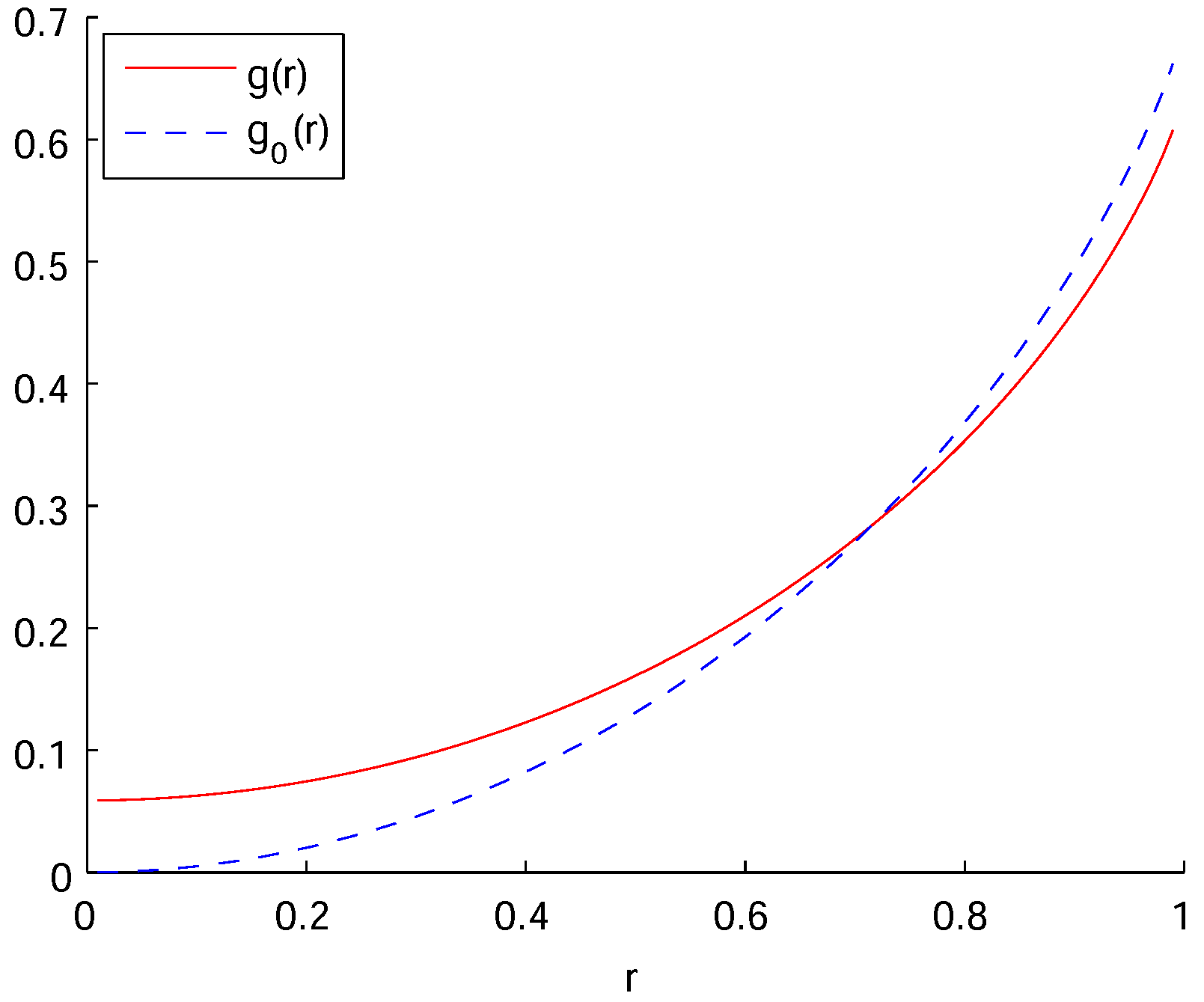
We note that the Bayesian predictive density operator is identical for every ${\pi }^{\ast }\in {\mathcal{P}}_{1-\mathrm{qubit}}^{\ast }$. In fact, every ${\pi }^{\ast }\in {\mathcal{P}}_{1-\mathrm{qubit}}^{\ast }$ also provides the minimax estimation of density operator ${\sigma }_{\theta }^Y$ when there is no observation system X. Figure 1 shows the risk function $g(r)$ in (17) and also the minimax risk function $g_0(r)$ when there is no observation:

$$\begin{array}{cc}\hfill g_0(r)& =\mathrm{Tr}\left(\left(\begin{array}{cc}(1+r)/2& 0\\ 0& (1-r)/2\end{array}\right)\left(\log \left(\begin{array}{cc}(1+r)/2& 0\\ 0& (1-r)/2\end{array}\right)-\log \left(\begin{array}{cc}1/2& 0\\ 0& 1/2\end{array}\right)\right)\right)\hfill \\ & =-h(r)+\log 2.\hfill \end{array}$$

Whereas $g(r)<g_0(r)$ around $r=1$, we can see that $g(r)>g_0(r)$ around $r=0$. Both risk functions take the maximum at $r=1$ and

$$g(1)=\log 3-(2/3)\log 2<g_0(1)=\log 2.$$

The decrease $g_0(1)-g(1)>0$ in the maximum risk corresponds to the gain from the observation X.

Now, we consider the selection of the measurement E. As we discussed in the previous section, we define a POVM $E^{\ast }$ to be a minimax POVM if it satisfies (13). We provide a sufficient condition on a POVM to be minimax. Let ${\rho }^E$ be a minimax predictive density operator for the measurement E.

Lemma 5.

Suppose ${\pi }^{\ast }$ is a latent information prior for the measurement $E^{\ast }$. If

$$\begin{array}{c}\hfill \int R_{E^{\ast }}(\theta ,{\rho }^{E^{\ast }})\mathrm{d}{\pi }^{\ast }(\theta )=\underset{E}{\inf }\int R_E(\theta ,{\rho }^E)\mathrm{d}{\pi }^{\ast }(\theta ),\end{array}$$

then $E^{\ast }$ is a minimax POVM.

Proof. 

For every $(E,\rho )$, we have

$$\begin{array}{cc}\hfill \underset{\theta }{\sup }{R}_E(\theta ,\rho )& \ge \underset{\rho }{\inf }\underset{\theta }{\sup }{R}_E(\theta ,\rho )=\underset{\theta }{\sup }{R}_E(\theta ,{\rho }^E)\hfill \\ & =\int R_E(\theta ,{\rho }^E)\mathrm{d}{\pi }^{\ast }(\theta )\ge \underset{E}{\inf }\int R_E(\theta ,{\rho }^E)\mathrm{d}{\pi }^{\ast }(\theta )\hfill \\ & =\int R_{E^{\ast }}(\theta ,{\rho }^{E^{\ast }})\mathrm{d}{\pi }^{\ast }(\theta )=\underset{\theta }{\sup }{R}_{E^{\ast }}(\theta ,{\sigma }_{{\pi }^{\ast }}).\hfill \end{array}$$

The last equality is from the minimaxity of ${\sigma }_{{\pi }^{\ast }}$. Therefore, $E^{\ast }$ is a minimax POVM. ☐

Theorem 4.

Every $E^{\ast }\in {\mathcal{E}}_{1-\mathrm{qubit}}^{\ast }$ is a minimax POVM.

Proof. 

Let ${\pi }^{\ast }\in {\mathcal{P}}_{1-\mathrm{qubit}}^{\ast }$. From Theorem 6, ${\pi }^{\ast }$ is a latent information prior for $E^{\ast }$.

For general measurement E, from Lemma 4, the risk function of the Bayesian predictive density operator ${\sigma }_{{\pi }^{\ast }}$ is

$$\begin{array}{cc}\hfill R_E(\theta ,{\sigma }_{{\pi }^{\ast }})=& -h\left(\frac{1+\parallel \theta \parallel }{2}\right)+\frac{1}{2}\log \frac{9}{2}-\frac{\log 2}{2}({{\theta }_x}^2{E}_{\mu }[x^2]+{{\theta }_y}^2{E}_{\mu }[y^2]+{{\theta }_z}^2{E}_{\mu }[z^2]\hfill \\ & +2{\theta }_x{\theta }_y{E}_{\mu }[xy]+2{\theta }_y{\theta }_z{E}_{\mu }[yz]+2{\theta }_z{\theta }_x{E}_{\mu }[zx]).\hfill \end{array}$$

Hence, the Bayes risk of ${\sigma }_{{\pi }^{\ast }}$ with respect to ${\pi }^{\ast }$ is

$$\begin{array}{c}\hfill \int R_E(\theta ,{\sigma }_{{\pi }^{\ast }})\mathrm{d}{\pi }^{\ast }(\theta )=\log 3-\frac{2}{3}\log 2.\end{array}$$

Now, since the Bayesian predictive density operator ${\sigma }_{{\pi }^{\ast }}$ minimizes the Bayes risk with respect to ${\pi }^{\ast }$ among all predictive density operators [4],

$$\begin{array}{c}\hfill \int R_E(\theta ,{\rho }^E)\mathrm{d}{\pi }^{\ast }(\theta )\ge \int R_E(\theta ,{\sigma }_{{\pi }^{\ast }})\mathrm{d}{\pi }^{\ast }(\theta )=\log 3-\frac{2}{3}\log 2\end{array}$$

for every E. Therefore,

$$\begin{array}{c}\hfill \underset{E}{\inf }\int R_E(\theta ,{\rho }^E)\mathrm{d}{\pi }^{\ast }(\theta )\ge \log 3-\frac{2}{3}\log 2.\end{array}$$

On the other hand,

$$\begin{array}{c}\hfill \underset{E}{\inf }\int R_E(\theta ,{\sigma }_{{\pi }^{\ast }})\mathrm{d}{\pi }^{\ast }(\theta )\le \int R_{E^{\ast }}(\theta ,{\sigma }_{{\pi }^{\ast }})\mathrm{d}{\pi }^{\ast }(\theta )=\log 3-\frac{2}{3}\log 2\end{array}$$

is obvious.

Hence,

$$\begin{array}{c}\hfill \int R_{E^{\ast }}(\theta ,{\sigma }_{{\pi }^{\ast }})\mathrm{d}{\pi }^{\ast }(\theta )=\underset{E}{\inf }\int R_E(\theta ,{\sigma }_{{\pi }^{\ast }})\mathrm{d}{\pi }^{\ast }(\theta )=\log 3-\frac{2}{3}\log 2.\end{array}$$

From Lemma 5, $E^{\ast }$ is minimax. ☐

Whereas Theorems 1 and 2 are valid even when ${\sigma }_{\theta }^{XY}$ is not separable, Theorems 3 and 4 assume the separability ${\sigma }_{\theta }^{XY}={\sigma }_{\theta }^X\otimes {\sigma }_{\theta }^Y$.

From Theorem 4, the POVM (15) is a minimax POVM. Since this POVM is identical to the SIC-POVM [14,15], it is an interesting problem whether the SIC-POVM is a minimax POVM also in higher dimensions. This is a future work.

References

- Barndorff-Nielsen, O.E.; Gill, R.D.; Jupp, P.E. On quantum statistical inference. J. R. Stat. Soc. B 2003, 65, 775–804. [Google Scholar] [CrossRef]
- Holevo, A.S. Probabilistic and Statistical Aspects of Quantum Theory; Elsevier: Amsterdam, The Netherlands, 1982. [Google Scholar]
- Paris, M.; Rehacek, J. Quantum State Estimation; Springer: Berlin, Germany, 2004. [Google Scholar]
- Tanaka, F.; Komaki, F. Bayesian predictive density operators for exchangeable quantum-statistical models. Phys. Rev. A 2005, 71, 052323. [Google Scholar] [CrossRef]
- Tanaka, F. Bayesian estimation of the wave function. Phys. Lett. A 2012, 376, 2471–2476. [Google Scholar] [CrossRef]
- Tanaka, F. Noninformative prior in the quantum statistical model of pure states. Phys. Rev. A 2012, 85, 062305. [Google Scholar] [CrossRef]
- Geisser, S. Predictive Inference: An Introduction; Chapman & Hall: London, UK, 1993. [Google Scholar]
- Csiszar, I. Axiomatic characterizations of information measures. Entropy 2008, 10, 261–273. [Google Scholar] [CrossRef]
- Aitchison, J. Goodness of prediction fit. Biometrika 1975, 62, 547–554. [Google Scholar] [CrossRef]
- Komaki, F. Bayesian predictive densities based on latent information priors. J. Stat. Plan. Inference 2011, 141, 3705–3715. [Google Scholar] [CrossRef]
- Bernardo, J.M. Reference posterior distributions for Bayesian inference. J. R. Stat. Soc. B 1979, 41, 113–147. [Google Scholar]
- Petz, D. Quantum Information and Quantum Statistics; Springer: New York, NY, USA, 2008. [Google Scholar]
- Holevo, A.S. Quantum Systems, Channels, Information: A Mathematical Introduction; Walter de Gruyter: Berlin, Germany, 2013. [Google Scholar]
- Appleby, D.M. SIC-POVMs and the extended Clifford group. J. Math. Phys. 2004, 46, 547–554. [Google Scholar]
- Renes, J.M.; Blume-Kohout, R.; Scott, A.J.; Caves, C.M. Symmetric informationally complete quantum measurements. J. Math. Phys. 2004, 45, 2171–2180. [Google Scholar] [CrossRef]
- Ferrie, C.; Blume-Kohout, R. Minimax quantum tomography: Estimators and relative entropy bounds. Phys. Rev. Lett. 2016, 116, 090407. [Google Scholar] [CrossRef] [PubMed]
- Tanaka, F. Quantum minimax theorem. arXiv 2014, arXiv:1410:3639. [Google Scholar]
- Billingsley, P. Convergence of Probability Measures; Wiley: New York, NY, USA, 1999. [Google Scholar]
- Hiai, F.; Petz, D. Introduction to Matrix Analysis and Applications; Springer: New York, NY, USA, 2014. [Google Scholar]
- Haapasalo, E.; Heinosaari, T.; Pellonpää, J.P. Quantum measurements on finite dimensional systems: Relabeling and mixing. Quantum Inf. Process. 2012, 11, 1751–1763. [Google Scholar] [CrossRef]
Figure 1.
Risk functions of predictive density operators. solid line: , dashed line: .
© 2017 by the authors. Licensee MDPI, Basel, Switzerland. This article is an open access article distributed under the terms and conditions of the Creative Commons Attribution (CC BY) license (http://creativecommons.org/licenses/by/4.0/).
Share and Cite
MDPI and ACS Style
Koyama, T.; Matsuda, T.; Komaki, F. Minimax Estimation of Quantum States Based on the Latent Information Priors. Entropy 2017, 19, 618. https://doi.org/10.3390/e19110618
AMA Style
Koyama T, Matsuda T, Komaki F. Minimax Estimation of Quantum States Based on the Latent Information Priors. Entropy. 2017; 19(11):618. https://doi.org/10.3390/e19110618
Chicago/Turabian StyleKoyama, Takayuki, Takeru Matsuda, and Fumiyasu Komaki. 2017. "Minimax Estimation of Quantum States Based on the Latent Information Priors" Entropy 19, no. 11: 618. https://doi.org/10.3390/e19110618
Note that from the first issue of 2016, this journal uses article numbers instead of page numbers. See further details here.