Paradigms of Cognition †

Department of Mathematical Sciences, University of Copenhagen, Universitetsparken 5, 2100 Copenhagen, Denmark
†
This paper is an extended version of our paper published in the 36th International Workshop on Bayesian Inference and Maximum Entropy Methods in Science and Engineering, Ghent, Belgium, 10–15 July 2016.
Entropy 2017, 19(4), 143; https://doi.org/10.3390/e19040143
Submission received: 19 December 2016
/
Revised: 23 February 2017
/
Accepted: 10 March 2017
/
Published: 27 March 2017
(This article belongs to the Special Issue Selected Papers from MaxEnt 2016)
Abstract
:An abstract, quantitative theory which connects elements of information—key ingredients in the cognitive proces—is developed. Seemingly unrelated results are thereby unified. As an indication of this, consider results in classical probabilistic information theory involving information projections and so-called Pythagorean inequalities. This has a certain resemblance to classical results in geometry bearing Pythagoras’ name. By appealing to the abstract theory presented here, you have a common point of reference for these results. In fact, the new theory provides a general framework for the treatment of a multitude of global optimization problems across a range of disciplines such as geometry, statistics and statistical physics. Several applications are given, among them an “explanation” of Tsallis entropy is suggested. For this, as well as for the general development of the abstract underlying theory, emphasis is placed on interpretations and associated philosophical considerations. Technically, game theory is the key tool.
Contents
| 1 | Introduction | 2 | |
| 2 | Information without Probability | 5 | |
| 2.1 | The World and You . . . . . . . . . . . . . . . . . . . . . . . . . . . . . . . . . . . . . | 5 | |
| 2.2 | Truth and Belief . . . . . . . . . . . . . . . . . . . . . . . . . . . . . . . . . . . . . . . . | 5 | |
| 2.3 | A Tendency to Act, a Wish to Control . . . . . . . . . . . . . . . . . . . . . . . | 6 | |
| 2.4 | Atomic Situations, Controllability and Visibility . . . . . . . . . . . . . . . | 7 | |
| 2.5 | Knowledge, Perception and Deformation . . . . . . . . . . . . . . . . . . . . | 8 | |
| 2.6 | Effort and Description . . . . . . . . . . . . . . . . . . . . . . . . . . . . . . . . . . . | 9 | |
| 2.7 | Information Triples . . . . . . . . . . . . . . . . . . . . . . . . . . . . . . . . . . . . . | 11 | |
| 2.8 | Relativization, Updating . . . . . . . . . . . . . . . . . . . . . . . . . . . . . . . . . | 15 | |
| 2.9 | Feasible Preparations, Core and Robustness . . . . . . . . . . . . . . . . . . | 16 | |
| 2.10 | Inference via Games, Some Basic Concepts . . . . . . . . . . . . . . . . . . | 18 | |
| 2.11 | Refined Notions of Properness . . . . . . . . . . . . . . . . . . . . . . . . . . . . | 21 | |
| 2.12 | Inference via Games, Some Basic Results . . . . . . . . . . . . . . . . . . . . | 22 | |
| 2.13 | Games Based on Utility, Updating . . . . . . . . . . . . . . . . . . . . . . . . . . | 28 | |
| 2.14 | Formulating Results with a Geometric Flavour . . . . . . . . . . . . . . . . | 29 | |
| 2.15 | Adding Convexity . . . . . . . . . . . . . . . . . . . . . . . . . . . . . . . . . . . . . . | 32 | |
| 2.16 | Jensen-Shannon Divergence at Work . . . . . . . . . . . . . . . . . . . . . . . . | 36 | |
| 3 | Examples, towards Applications | 42 | |
| 3.1 | Primitive Triples and Generation by Integration . . . . . . . . . . . . . . . | 42 | |
| 3.2 | A Geometric Model . . . . . . . . . . . . . . . . . . . . . . . . . . . . . . . . . . . . . | 48 | |
| 3.3 | Universal Coding and Prediction . . . . . . . . . . . . . . . . . . . . . . . . . . . | 50 | |
| 3.4 | Sylvester’s Problem from Location Theory . . . . . . . . . . . . . . . . . . . | 52 | |
| 3.5 | Capacity Problems, an Indication . . . . . . . . . . . . . . . . . . . . . . . . . . | 53 | |
| 3.6 | Tsallis Worlds . . . . . . . . . . . . . . . . . . . . . . . . . . . . . . . . . . . . . . . . . . | 54 | |
| 3.7 | Maximum Entropy Problems of Classical Shannon Theory . . . . . . | 58 | |
| 3.8 | Determining D-Projections . . . . . . . . . . . . . . . . . . . . . . . . . . . . . . . | 60 | |
| 4 | Conclusions | 61 | |
| A | Notions of Properness | 62 | |
| B | Protection against Misinformation | 65 | |
| C | Cause and Effect | 66 | |
| D | Negative Definite Kernels and Squared Metrics | 66 | |
1. Introduction
Originally, the driving force behind this study was to extend the clear and convincing operational interpretations associated with classical information theory as developed by Shannon [1] and followers, to the theory promoted by Tsallis for statistical physics and thermodynamics, cf., [2,3]. That there are difficulties is witnessed by the fact that, despite its apparent success, some well known physicists still find grounds for criticism. Evidence of this attitude may be found in Gross [4].
A possible solution to the problem is presented towards the end of our study, in Theorem 18. It is based on the idea that, possibly, what the physicist perceives as the essence in a particular situation could be a result of both the true state of the situation and the physicists preconceptions as expressed by his beliefs. In case there is no deformation from truth and belief to perception, i.e., if “what you see is what is true”, you regain the classical notions of Boltzmann, Gibbs and Shannon.
The approach indicated in Theorem 18 rests on philosophical considerations and associated interpretations. As it turns out, this approach is applicable in a far more abstract setting than needed for the discussion of the particular problem. As a result, a general abstract, quantitative theory is developed. This theory, presented in Section 2, with its many subsections is the main contribution of our research. A number of possible applications, including Theorem 18, are listed in Section 3, which has a number of sub-sections covering applications from different areas. They serve as justification for the work which has gone into the development of the general abstract theory. The conclusions are collected in Section 4.
The theory may be seen as an extension of classical Shannon theory. One does not achieve the same degree of clarity as in the classical theory, where coding provides a solid reference. However, the results developed in Section 2 and Section 3 demonstrate that the extension to a more abstract framework is meaningful and opens up for new areas of research. In addition, previous results are consolidated and unified.
The theory of Section 2 is an abstract theory of information without probability. Inspiration from Shannon Theory and from the theory of inference within statistics and statistical physics is apparent. However, the ideas are presented here as an independent theory.
Previous endeavours in the direction taken include research by Ingarden and Urbanik [5] who wrote “... information seems intuitively a much simpler and more elementary notion than that of probability ... [it] represents a more primary step of knowledge than that of cognition of probability ...”. We also point to Kolmogorov, cf., [6,7] who in the latter reference (but going back to 1970, it seems) stated “Information theory must precede probability theory and not be based on it”. The ideas by Ingarden and Urbanik were taken up by Kampé de Fériet, see the survey in [8]. The work of Kampé de Fériet is rooted in logic. Logic is also a key ingredient in comprehensive studies over some 40 years by Jaynes, collected posthumously in [9]. Although many philosophically-oriented discussions are contained in the work of Jaynes, the situations he deals with are limited to probabilistic models and intended mainly for a study of statistical physics.
The work by Amari and Nagaoka in information geometry, cf., [10], may also be viewed as a broad attempt to free oneself from a tie to probability. There are many followers of the theory developed by Amari and Nagaoka. Here we only mention the recent thesis by Anthonis [11] which has a base in physics.
In complexity theory as developed by Solomonoff, Kolmogorov and others, cf., the recent survey [12] by Rathmanner and Hutter, we have a highly theoretical discipline which aims at inference not necessarily tied to probabilistic modeling. The Minimum Description Length Principle may be considered an important spin-off of this theory. It is mainly directed at problems of statistical inference and was developed, primarily, by Rissanen and by Barron and Yu, cf., [13]. We also point to the treatise [14] by Grünwald. In this work you find discussions of many of the issues dealt with here, including a discussion of the work of Jaynes.
Still other areas of research have a bearing on “information without probability”, e.g., semiotics, philosophy of information, pragmatism, symbolic linguistics, placebo research, social information and learning theory. Many areas within psychology are also of relevance. Some specific works of interest include Jumarie [15], Shafer and Vovk [16], Gernert [17], Bundesen and Habekost [18], Benedetti [19] and Brier [20]. The handbook [21] edited by Adriaans and Bentham and the encyclopaedia article [22] by Adriaans collect views on the very concept of “information”. Over the years, an overwhelming amount of thought has been devoted to that concept in one form or another. Most of this bulk of material is entirely philosophical and not open to quantitative analysis. Part of it is impractical and presently mainly of theoretical interest. Moreover, some is far from Shannon’s theory which we hold as a cornerstone of quantitative information theory. In fact, we consider it a requirement of any quantitative theory of information to be downward compatible with basic parts of Shannon theory. This requirement is largely respected in the present work, but not entirely. For example, we do not know if one can meaningfully lift the concept of coding as known from Shannon theory to a more abstract level.
In many respects, our endeavours go “beyond Shannon”. So does, e.g., Brier in his development of cybersemiotics, cf., [20,23]. Brier goes deeper into some of the philosophical aspects than we do and also attempts a broad coverage by incorporating not only the exact natural sciences but also life science, the humanities and the social sciences. Though not foreign to such a wider scope, our study aims at more concrete results by basing the study more directly on quantitative elements. Both studies emphasize the role of the individual in the cognitive process.
A special feature of our development is the appeal to game theoretical considerations, cf., especially Section 2.10, Section 2.12 and Section 2.13. To illuminate the importance we attach to this aspect we quote from Jaynes’ preface to [9] where he comments on the maximum entropy principle, the central principle of inference promoted by Jaynes:
“... it [maximum entropy] predicts only observable facts (functions of future or past observations) rather than values of parameters which may exist only in our imagination ... it protects us against drawing conclusions not warranted by the data. But when the information is extremely vague, it may be difficult to define any appropriate sample space, and one may wonder whether still more primitive principles than maximum entropy can be found. There is room for much new creative thought here.”
This is one central place where game theory comes in. It represents a main addition, so we claim, to Jaynes’ work In passing, it is noted that at the conference “Maximum Entropy and Bayesian Methods”, Paris 1992, the author had much hoped to discuss the impact of game theoretical reasoning with professor Jaynes. Unfortunately, Jaynes, who died in 1998, was too ill at the time to participate. He never incorporated arguments such as those in [24] which can be conceived as supportive of his own theory.
The merits of game theory in relation to information theoretical inference were first indicated in the probabilistic, Shannon-like setting, independently of each other, by Pfaffelhuber [25] and by the author [26]. More recent references include Harremoës and Topsøe [27], Grünwald and Dawid [28], Friedman et al. [29] (a utility-based work) and Dayi [30]. As sources of background material [31,32,33] may be helpful.
The quantitative elements we work with are brought into play via a focus on description effort—or just effort. From this concept, general notions of entropy and redundancy (and the close to equivalent notion of divergence) are derived. The information triples we shall take as the key object of study are expressions of the concepts effort/entropy/redundancy (or effort/entropy/divergence). By a “change of sign”, the triples may, just as well, concern utility/max-utility/divergence.
Apart from introducing game theory into the picture, a main feature of the present work lies in its abstract nature with a focus on interpretations rather than on axiomatics which was the emphasis of many previous authors, including Jaynes.
The set of interpretations we shall emphasize in Section 2 is not be the only one possible. Different sets of interpretations are briefly indicated in Appendix B and Appendix C. Though some of this played a role in the development, in statistics, of the notion of properness, we have relegated the material to the appendices, not to disturb the flow of presentation and also as we consider this material to be of lesser significance when comparing it with the main line of thought.
Section 3 may be viewed as a justification of the partly speculative deliberations of Section 2.1, Section 2.2, Section 2.3, Section 2.4, Section 2.5, Section 2.6, Section 2.7, Section 2.8, Section 2.9, Section 2.10, Section 2.11, Section 2.12, Section 2.13, Section 2.14, Section 2.15 and Section 2.16. Also, in view of the rather elaborate theory of Section 2 with many new concepts and unusual notation, it may well be that occasional reference to the material in Section 3 will ease the absorption of the theoretical material.
In Section 3.1, the natural building stones behind the information triples is presented. This is closely related to the well-known construction associated with Bregman’s name. The construction may be expanded by allowing non-smooth functions as “generators”. Pursuing this leads to situations where the standard notion of properness breaks down and needs a replacement by weaker notions. Such notions are introduced at the end of Section 2.10 but may only be appreciated after acquaintance with the less abstract material in Appendix A.
The applications presented—or indications of potential applications—come from combinatorial geometry, probabilistic information theory, statistics and statistical physics. For most of them, we focus on providing the key notions needed for the theory to work, thus largely leaving concrete applications aside. The aim is to provide enough details in order to demonstrate that our modeling can be applied in quite different contexts. For the case of discrete probabilistic models we do, however, embark on a more thorough analysis. The reason for this is, firstly, that this is what triggered the research reported on and, secondly, with a thorough discussion of modeling in this context, virtually all elements introduced in the many sub-sections of Section 2 have a clear and natural interpretation. In fact, full appreciation of the abstract theory may only be achieved after reading the material in Section 3.6 and Section 3.7.
Our treatment is formally developed independently of previous research. However, unconsciously or not, it depends on earlier studies as referred to above and on the tradition developed over time. More specifically, we mention that our focus on description effort, especially the notion of properness, cf., Section 2.6, is closely related to ideas first developed for areas touching on meteorology, statistics and information theory.
Previous relevant writings of the author include [34,35,36,37,38]. The present study is here published as a substantial expansion of the latter. For instance, elements related to control—modeling an observer’s active response to belief—and a detailed discussion of Jensen-Shannon divergence as well as more cumbersome technical details were left out in [38]. Thus, [38] may best serve as an easy-to-read appetizer to the present more heavy and comprehensive theory.
2. Information without Probability
2.1. The World and You
By we denote the actual world, perhaps one among several possible worlds. Two fictitious persons play a major role in our modeling, “Nature” and “Observer”. These “persons” behave quite differently and, though stereotypical, the reader may associate opposing sexes to them, say female for Nature, male for Observer. The interplay between the two takes place in relation to studies of situations from the world. Observer’s aim is to gain insight about situations studied. It may be helpful to think of Observer as “you”, say a physicist, psychologist, statistician, information theoretician or what the case may be. Nature is seen as an expression of the world itself and reflects the rules of the world. Mostly, such rules may be identified with laws of nature. However, we shall consider models where the rules express an interplay between Nature and Observer and as such may not be absolutes, independent of observer’s interference.
The insight or knowledge sought by Observer will be focused on inference concerning particular situations under study. A different form of inference not focused on any particular situation may also be of relevance if Observer does not know which world he is placed in. Of course, the actual world is a possible world or it could not exist. So Observer may, based on experience gained from situations encountered, attempt to ascertain which one out of a multitude of possible worlds is actualized.
The notions introduced are left as loose indications. They will take more shape as the modeling progresses. The terminology chosen here and later on is intended to provoke associations to common day experiences of the cognitive process. In addition, the terminology is largely consistent with usage in philosophy.
2.2. Truth and Belief
Nature is the holder of truth. Observer seeks the truth but is relegated to belief. However, Observer possesses a conscious and creative mind which can be exploited in order to obtain knowledge as effortlessly as possible. In contrast, Nature does not have a mind—and still, the reader may find it helpful to think of Nature as a kind of “person”!
We introduce a set X, the state space, and a set Y, the belief reservoir. Elements of X, generically denoted by x, are truth instances or states of truth or just states, whereas elements of Y, generically denoted by y, are belief instances. We assume that . Therefore, in any situation, it is conceivable that Observer actually believes what is true. Mostly, will hold. Then, whatever Observer believes, could be true.
Typically, in any situation, we imagine that Nature chooses a state and that Observer chooses a belief instance. This leads to the introduction of certain games which will be studied systematically later on, starting with Section 2.10.
Though there may be no such thing as absolute truth, it is tempting to imagine that there is and to think of Natures choice as an expression of just that. This then helps to maintain a distinction between Nature and Observer. However, a closer analysis reveals that what goes on at Natures side is most correctly thought of as another manifestation of Observer. Thus the two sides cannot be separated. Rather, a key to our modeling is the interplay between the two.
For some models it may be appropriate to introduce a set of realistic states. States not in are considered unrealistic, out of reach for Observer, typically because they would involve availability of unlimited resources. Moreover, some models involve a set of certain beliefs. Beliefs from are chosen by Observer if he is quite determined on what is going on—but of course, he could be wrong. If nothing is said to the contrary, you can take and .
In a specific situation, Nature’s choice may not be free within all of X. Rather, it may be restricted to a non-empty subset of X, the preparation. The idea is that Observer, perhaps a physicist, can “prepare” a situation, thereby forcing Nature to restrict the choice of state accordingly. For instance, by placing a gas in a heat bath, Nature is restricted to states which have a mean energy consistent with the prescribed temperature.
A situation is normally characterized by specifying a preparation . A state x is consistent—viz., consistent with the preparation of the situation—if . Later on, we shall consider preparation families which are sets, generically denoted by , whose members are preparations.
Faced with a specific situation with preparation , Observer speculates about the state of truth chosen by Nature. Observer may express his opinion by assigning a belief instance to the situation. If this is always chosen from the preparation , Observer will only believe what could be true. Sometimes, Observer may prefer to assign a belief instance in Y\P to the situation. Then this instance cannot possibly be one chosen by Nature. Nevertheless, it may be an adequate choice if an instance inside would contradict Observer’s subjective beliefs. Therefore, the chosen instance may be the “closest” to the actual truth instance in a subjective sense. Anyhow, Observer’s choice of belief instance is considered a subjective choice which takes available information into account such as general insight and any prior information. Qualitatively, these thoughts agree with Bayesian thinking, and as such enjoy the merits, but are also subject to the standard criticism, which applies to this line of thought, cf., [12,39].
2.3. A Tendency to Act, a Wish to Control
Two considerations will lead us to new and important structural elements.
First, we point to the mantra that belief is a tendency to act. This is a rewording taken from Good [40] who suggested this point of view as a possible interpretation of the notion of belief. In daily life, action appears more often than not to be a spontaneous reaction in situations man is faced with, rather than a result of rational considerations. Or reaction depends on psychological factors or brain activity largely outside conscious control. In contrast, we shall rely on rational thinking based on quantitative considerations. As a preparation we introduce a set , the action space, and a map from Y into , referred to as response. Elements of are called actions. We use the notation to indicate the action which is Observer’s response in situations where Observer’s belief is represented by the belief instance y. Note that as we have assumed that , is well defined for every state x.
Response need not be injective, thus it is in general not possible to infer Observer’s belief from Observer’s action. Response need not either be surjective, though for most applications it will be so. Actions not in the range are idle for the actual model under discussion but may become relevant if the setting is later expanded.
Belief instances, say and , with the same response are response-equivalent, notationally written .
If the model contains certain beliefs, i.e., if , we assume that contains a special element, the empty action, and that this action is chosen by Observer in response to any certain belief instance. In such cases, Observer sees no reason to take any action. If Observer finds several actions equally attractive, one could allow response to be a set-valued map. However, for the present study we insist that response is an ordinary map defined on all of Y. This will actually be quite important.
For a preparation , denotes the set of with .
Let us turn to another tendency of man, the wish to control. This makes us introduce a set W, the control space. The elements of W are referred to as controls. For the present modeling, this will not, formally, lead to further complications as we shall take W and to be identical: . This simplification may be defended by taking the point of view that in order to exercise control, you have to act, typically by setting up appropriate experiments. Moreover, you may consider it the purpose of Observer’s action to exercise control. Thus, in an idealized and simplified model as here presented, we simply identify the two aspects, action and control. Later elaborations of the modeling may lead to a clear distinction between action and the more passive concept of control. As and W are identified, we shall often use w as a generic element of and we shall denote the empty action—the same as the empty control—by .
The simplest models are obtained when response is an injection or even a bijection. Moreover, simplest among these models are the cases when and response is the identity map. This corresponds to a further identification of belief with action or control. Even then it makes a difference if you think about an element as an expression of belief, as an expression of action or as an expression of control.
Although many models do not need the introduction of (or W), the further development will to a large extent refer first and foremost to -related concepts. Technically, this results in greater generality, as response need not be injective. Belief-type concepts, often indicated by referring to the “Y-domain”, will then be derived from action- or control-based concepts, often indicated by pointing to the “-domain”. The qualifying indication may be omitted if it is clear from the context whether we work in the one domain or the other.
2.4. Atomic Situations, Controllability and Visibility
Two relations will be introduced. Controllability is the primary one from which the other one, visibility, will be derived. These relations constitute refinements which may be disregarded at a first reading. This can be done by taking the relations to be the diffuse relations , in notation below, and . The reader may recall that in general mathematical jargon, a diffuse relation is one without restrictions, i.e., one for which any element is in relation to any other element.
Pairs of states and belief instances or pairs of states and controls are key ingredients in situations from the world. However, not all such pairs will be allowed. Instead, we imagine that offhand, Observer has some limited insight into Natures behaviour and therefore, Observer takes care not to choose “completely stupid” belief instances or controls, as the case may be.
We express these ideas in the -domain by introducing a relation from X to , called controllability and denoted . Thus is a subset of the product set . Elements of are atomic situations (in the -domain). If a preparation is given, it may suffice to consider the restriction which consists of all atomic situations with .
For an atomic situation , we write and say that w controls x or that x can be controlled by w. An atomic situation is an adapted pair if w is adapted to x in the sense that .
For a preparation we write , and call w a control of , if w controls every state in (). We also express this by saying that w controls . By we denote the set of all controls of . We write if is the singleton set . In case is the diffuse relation, for any preparation .
For , denotes the control region of , the set of for which for some . We write if is the singleton set . Clearly, the statements , and are equivalent.
We assume that the following conditions hold:
and normally also that
The first condition is essential and the second one is rather innocent. The third condition is introduced when we want to ensure that X (or Y) is not “too large”. Models where (3) does not hold are considered unrealistic, beyond what man (Observer) can grasp. If response is surjective, it amounts to the condition . It is illuminating to have models of classical Shannon theory in mind, cf., Section 3.7.
For a preparation , we define the centre of (-domain) as the set of controls in which control :
From controllability we derive the relation of visibility for the Y-domain, denoted , and given by
Restrictions are at times of relevance.
If , we say that is an atomic situation (in the Y-domain) and write . Such a situation is an adapted pair if is so in the -domain, i.e., if and is a perfect match if . The two notions coincide if response is injective. An atomic situation is certain if .
Note that we use the same sign, ≻, for visibility and for controllability. The context will have to show if we work in the Y- or in the -domain. We see that if and only if . If this is so, we also say that y covers x or that x is visible from y.
By (1) and by the defining relation (5), for all , thus contains the diagonal . The outlook (or view) from is the set . Clearly, . By (2) and (5), this set is non-empty and, when (3) holds, for at least one belief instance, the outlook is all of X.
For a preparation we write , and call y a viewpoint of , if for every . The set of all viewpoints of is denoted . We write if is the singleton . By , the centre of (Y-domain), we denote the set of viewpoints in the preparation:
Note that .
In any situation, Observer should ensure that from his chosen belief instance, every state which could conceivably be chosen by Nature is visible. Therefore, in a situation where the preparation is known to Observer, Observer should only consider belief instances in .
In the sequel we shall often consider bivariate functions, generically denoted by either (-domain) or by f (Y-domain). The -type functions are defined either on or on some subset of the form for some preparation . The range of may be any abstract set but will often be a subset of the extended real line. Given , it is understood that f without the hat denotes the derived function defined by for pairs for which is in the domain of definition of . The domain of definition of the derived function is either or the set if is defined on .
Every derived function depends only on response in the sense that if only . If response is a surjection, there is a natural one-to-one relation between -type functions and Y-type functions which depend only on response.
Consider an f-type function defined on all of . For , denotes the marginal function given y, defined on by . The marginal function given is the function defined by for . We write on to express, firstly, that so that is well defined on all of and, secondly, that this marginal function is finite on . We write if on X.
2.5. Knowledge, Perception and Deformation
Observer strives for knowledge, conceived as the synthesis of extensive experience. Referring to probabilistic thinking, we could point to situations where accidental experimental data are smoothed out over time as you enter the regime of the law of large numbers. However, Observer’s endeavours may result in less definitive insight, a more immediate reaction which we refer to as perception. It reflects how Observer perceives situations from the world or, with a different focus, how situations from the world are presented to Observer.
In the same way as we have introduced truth- and belief instances, we consider knowledge instances, also referred to as perceptions. Typically, they are denoted by z and taken from a set denoted Z, the knowledge base or perception base.
A simplifying assumption for our modeling is that the rules of the world contain a special function, , which maps into Z, generically,
The derived function, , then maps into Z. Both functions are referred to as the deformation. The context will show which one we have in mind, or .
Thus knowledge can be derived deterministically from truth and belief alone, and as far as belief is concerned, we only have to know the associated response. In terms of perception, Observer’s perception z of an atomic situation is given by .
In our modeling, the world is characterized by the deformation. We may thus talk about the world with deformation , . The rules of the world may contain other structural elements, but such elements are not specified in the present study. Possibilities which could be considered in future developments include context, noise from the environment, and dynamics. To some extent, such features can be expressed in the present modeling by defining and Z appropriately and by introducing suitable interpretations.
In case response is a bijection and Z contains X as well as Y we may consider the deformations and defined by , respectively . The associated worlds are and . In , “what you see is what is true”, whereas in , “you only see what you believe”—or, in some interpretations, you only see what you want to see. The world is the classical world where, optimistically, truth can be learned, whereas, in , you cannot learn anything about truth. We refer to as a black hole. It is a narcissistic world, a world of extreme scepticism, only reflecting Observer’s beliefs and bearing no trace of Nature. If Z is provided with a linear structure, we can consider further deformations depending on a parameter q by putting . Worlds associated with deformations of this type are denoted . These are the worlds we find of relevance for the discussion of Tsallis entropy, cf., Section 3.6.
The simplest world to grasp is the classical world, but also the worlds and even a black hole contain elements which are familiar to us from daily experience, especially in relation to certain psychological phenomena. In this connection we point to placebo effects, cf., Benedetti [19], and to visual attention, cf., Bundesen and Habekost [18]. Presently, the relevance of our modeling in relation to these phenomena is purely qualitative.
Considering examples as indicated above, it is natural to expect that knowledge is of a nature closely related to the nature of truth and of belief. A key case to look into is that . However, we shall not make any general assumption in this direction. What we shall do is to follow the advice of Shannon, as far as possible avoiding assumptions which depend on concrete semantic interpretations. As a consequence we shall only in Section 3.6 introduce more specific assumptions about the representation of knowledge.
2.6. Effort and Description
We turn to the introduction of the key quantitative tool we shall work with. In so doing, we will be guided by the view that perception requires effort. Expressed differently, knowledge is obtained at a cost. Since, according to the previous section, knowledge can be derived from truth and belief alone, or from truth and action, no explicit reference to knowledge is necessary. Instead, we model effort (in the -domain) by a certain bivariate function, the effort function, defined on .
The rules of the world may not point directly to an effort function which Observer can favorably work with. Or there may be several sensible functions to choose from. The actual selection is considered a task for Observer.
Effort, description, experiment and measurement are related concepts. We put emphasis on the notion of description, which is intended to aid Observer in his encounters with situations from the world. Logically, description comes before effort. Effort arises when specific ideas about description are developed into a method of description, which you may here identify with an experiment. The implementation of such a method or the performance of the associated experiment involves a cost and this is what we conceive as specified quantitatively by the effort function.
Description depends on semantic interpretations and is often thought of in loose qualitative terms. However, in order to develop precise concepts which can be communicated among humans, quantitative elements will inevitably appear, typically through a finite set of certain real-valued functions, descriptors. The descriptors of Section 3.6 give an indication of what could be involved.
Imagine now that somehow Observer has chosen all elements needed—response, actions, experiments—and settled for an effort function, defined on . Let us agree on what a “good” effort function should mean. Generally speaking, Observer should aim at experiments with low associated effort. Consider a fixed truth instance x and the various possible actions, in principle free to be any action which controls x. It appears desirable that the action adapted to x should be the one preferred by Observer. Thus effort should be minimal in this case, i.e., should hold. Further, if the inequality is sharp except for the adapted action, this will have a training effect which, over time, will encourage Observer to choose the optimal action, .
Formally, we define an effort function (in the -domain) as a function on with values in such that, for all and all ,
Thus, for all , . The minimal value of is the entropy of x for which we use the notation :
This quantity will be discussed more thoroughly in the sequel. If , it is to be expected that when .
The effort function is proper, if, for any with , the minimum of is only achieved for the control adapted to x. As opposed to this notion we have the notion of a degenerate effort function which is one which only depends on the first argument x, i.e., for all , is a constant function.
Note that effort may be negative (but not ). This flexibility will later be convenient as it will allow us to pass freely from notions of effort to notions of utility by a simple change of sign. However, for more standard applications, effort functions will be non-negative.
The set of effort functions and the set of proper effort functions over are ordered positive cones in a natural way. You may note that if, in a sum of effort functions, one of the summands is proper, so is the sum. Two effort functions and , which only differ from each other by a positive finite factor are scalarly equivalent. If an effort function is proper, so is every scalarly equivalent one. There may be many non-scalarly equivalent effort functions. The choice among scalarly equivalent ones amounts to a choice of unit.
Proper effort functions could have been taken as the key primitive concept on which other concepts, especially response, can be based. To illustrate this, assume that and consider a function such that, for every state x for which is not identically , is a singleton. The minimal value of is again the entropy and we may define the set of realistic states by and, more importantly, response by the requirement that . This defines response uniquely on and for , the definition of is really immaterial and any element in which controls x will do.
Turning to the Y-domain, we define an effort function (Y-domain), as a function such that
Entropy is given by . If there are certain atomic situation, it is natural to expect that effort vanishes for such situations. The effort function is proper if equality in (10) only holds if either or else . We also express this by saying that satisfies the perfect match principle. An effort function is degenerate if, for every , .
The notions just introduced were defined directly with reference to the Y-domain. However, it lies nearby also to consider functions which can be derived from -effort functions . They are derived effort functions and, in case is proper, proper derived effort functions. The two strategies for definitions, intrinsic and via derivation, give slightly different concepts. In case response is injective, the resulting notions are equivalent. In general, derived effort functions depend only on response, i.e., if and and if then . In the other direction, for a proper derived effort function, you can only conclude response-equivalence, , if and .
Formally, the definitions related to Y-effort functions may be conceived as a special case of the definitions pertaining to the -domain (put and take the identity map as response).
We shall talk about effort functions without a qualifying prefix, or Y, if it is clear from the context what we have in mind. We shall always point out if we have derived functions in mind.
The effort functions introduced determine net effort. However, the implementation of the method of description—which we imagine lies behind—may, in addition to a specific cost, entail a certain overhead and, occasionally, it is appropriate to include this overhead in the effort. We refer to Section 3.6 for instances of this.
We imagine that the choice of effort function involves considerations related to knowledge and to the rules of the world. However, once , hence also are fixed, these other elements are only present indirectly. The ideas of Section 2.5 have thus mainly served as motivation for the further abstract development. The ideas will be taken up again when in Section 3.6 we turn to a study of probabilistic models.
The author was led to consider proper effort functions in order to illuminate certain aspects of statistical physics, cf., [34,37]. However, the ideas have been around for quite some time, especially among statisticians. For them it has been more natural to work with functions taken with the reverse sign by looking at “score” rather than effort. Our notion of proper effort functions, when specialized to a probabilistic setting, matches the notion of proper scoring rules as you find it in the statistical literature. As to the literature, Csiszár [41] comments on the early sources, including Brier [42], a forerunner of research which followed, cf., Good [40], Savage [43] (see e.g., Section 9.4) and Fischer [44]. See also the reference work [45] by Gneiting and Raftery. For research of Dawid and collaborators—partly in line with what you find here—see [28,46,47,48].
2.7. Information Triples
As advocated in the last section, effort is a notion of central importance. However, this notion should not stand alone but be discussed together with other fundamental concepts of information. This point of view will be emphasized by the introduction of a notion of information triples, the main notion of the present study. We start by philosophizing over the very concept of information.
Information in any particular situation concerns truth. If is a preparation, “” signifies that the true state is to be found among the states in . If is a singleton, we talk about full information and use the notation “x” rather than “”; otherwise, we talk about partial information.
We shall not be concerned with how information can be obtained—if at all. Perhaps, Observer only speculates about the potential possibility of acquiring information, either through his own activity or otherwise, e.g., via the involvement of an aid or a third party, an informer.
Information will be related to quantitatively defined concepts. As our basis we take a proper effort function . Following Shannon we disregard semantic content. Instead, we focus on the possibility for Observer to benefit from information by a saving of effort. Accordingly, we view as the information content of “x” in an atomic situation with x as truth instance and w as action or control—indeed, if you are told that x is the true state, you need not allocate the effort to the situation which you were otherwise prepared to do. The somewhat intangible and elusive concept of “information” is, therefore, measured by the more concrete and physical notion of effort, hence the unit of information is the same as the unit used for effort.
There is a huge literature elucidating what information really “is”. Suffice it here to refer to [21] and, as an example of a discussion more closely targeted on our main themes, we refer to Caticha [49] who maintains that “Just as a force is defined as that which induces a change in motion, so information is that which induces a change in beliefs”. One may just as well—or even better—focus on action. Then we can claim that “information” is that which induces a change of action.
The central concept of the theory developed by Shannon is that of entropy. This concept was already introduced in the preceding section. Here, we elaborate on possible interpretations. One view is that entropy is guaranteed saving of effort. With effort given by we are led to define the entropy associated with the information “x” as the minimum over w of . Thus, by (8), (9) holds.
The considerations above make most sense if, one way or another, Observer eventually obtains full information about the true state. However, if, instead, you view entropy as necessary allocation of effort, understood as the effort you have to allocate in order to have a chance to obtain full information, it does not appear important actually to obtain that information. In passing, one may think that a more neutral terminology such as “necessity” could have been chosen in place of “entropy”. That could be less awkward when you turn to other applications of the abstract theory than classical Shannon theory or statistical physics.
As yet a third route to entropy we suggest to view it as a quantitative expression of the complexity of the various states, maintaining that to evaluate complexity, Observer may use minimal accepted effort, the effort he is willing to allocate to the various states in order to obtain the information in question.
Entropy may also be obtained with reference only to the Y-domain. Indeed, with the derived effort function, for each state x, .
Whichever route to entropy you take—including the game theoretical route of Section 2.10—it appears that subjective elements are involved, typically through Observer’s choice of description and associated experiments. If, modulo scalar equivalence, the actual world only allows one proper effort function, then entropy and notions related to entropy are of a more objective nature. We shall later see examples of such worlds but also for such worlds subjective elements may enter if Observer is considering which world is the actual one.
Apart from effort itself, and the derived notion of entropy, we turn to the introduction of two other basic concepts which make sense in our abstract setting, viz., redundancy for the -domain and its counterpart, divergence, for the Y-domain.
To define redundancy, consider an atomic situation . Then redundancy between x and w is measured by the difference between actual and minimal effort, i.e., ideally, as
Assume, for a moment, that entropy is finite-valued. Then redundancy in (11) is well defined. Furthermore, redundancy is non-negative and only vanishes if is an adapted pair.
However, we find it important to be able to deal with models for which entropy may be infinite. We do that by simply assuming that appropriate versions of redundancy and divergence exist with desirable properties. The simple device we shall apply in order to reach a sensible definition is to rewrite the defining relation (11), isolating effort on the left hand side.
With the above preparations, we are ready to introduce the key concepts of our study. We start with concepts for the -domain and follow up after that by parallel concepts for the Y-domain.
We consider certain triples of functions taking values in with and defined on and H defined on X. If need be we may talk about triples over or we may point to the -domain. Such triples must satisfy special conditions in order to be of interest. The most important properties to consider are the following four:
The properties (12), (13) and (15) are considered for all and (14) for all . The linking identity (12) may be written shortly as or, formally correct with the projection of onto X, as .
An information triple is a triple which satisfies the three first conditions (L, F and S). For such triples the function is the associated effort function, H the associated entropy and the associated redundancy. This does not conflict with previous terminology. In particular, the associated effort function is indeed an effort function in the sense of Section 2.6.
Information triples with the same redundancy are said to be equivalent. Equivalent triples may have quite different properties and one may search for representatives with good properties.
A proper information triple in the Y-domain is an information triple for which redundancy is proper, i.e., (15) holds. Clearly, the effort function of a proper information triple is proper in the sense of Section 2.6. Moreover, if a triple is proper, so is any equivalent one.
An information triple is degenerate if redundancy vanishes: for all . The effort function of a degenerate information triple is degenerate.
Among the four defining properties, the last three (FSP) only involve redundancy. Accordingly, a function defined on is a general redundancy function if it satisfies the fundamental inequality as well as the requirements of soundness and properness. Note that for such a redundancy function, is a proper information triple and that any equivalent information triple may be obtained from by a natural process of addition related to any function on X with values in , taking this function as the entropy function. To be precise, what is involved structurally is that you add information triples, one of which is proper and the other degenerate, viz., you add and . For further details on this theme, see Section 3.1.
Normally, given a proper effort function , there is a natural way to extend the redundancy function as defined by (11) when , so that a proper information triple emerges. For this reason, we may talk about the information triple generated by . Then, the problem of indeterminacy of redundancy disappears. The slightly strengthened assumption that redundancy can be defined “appropriately” on all of will, as it turns out, present no limitation in concrete cases of interest.
We turn briefly to Y-type triples. They are triples with and D defined on and H defined on X. Key properties to consider are quite parallel to what we have discussed for the -domain:
An information triple in the Y-domain is a triple which satisfies the conditions L, F and S. For such triples, is the associated effort, H the associated entropy and D the associated divergence.
A proper information triple is one for which divergence is proper. Such triples are intrinsically defined in the sense that they do not depend on any action space or response function. If divergence vanishes, the triple is degenerate. The effort function of a proper information triple is proper in the sense of Section 2.6 and the effort function of a degenerate triple is degenerate.
A triple is a derived information triple, respectively a derived proper information triple, if there exists a triple satisfying the corresponding properties for the -domain such that is derived from and D from . Note that a derived proper information triple need not be a proper information triple according to the intrinsic definition. Indeed, from you can only conclude that x and y are response equivalent. Of course, if response is injective, the two types of proper information triples for the Y-domain—intrinsically defined or defined via derivation—are equivalent concepts.
A general divergence function D on is a function on which satisfies the F, S and P-requirements. Note that we include the property of properness in the definition. A general derived divergence function is one which can be derived from a general redundancy function.
For the Y-domain, notions of equivalence (same divergence!) and of addition of information triples are defined in the obvious manner.
Instead of taking triples as introduced above as the basis, it is quite often more natural to focus on triples of the “opposite nature”. This refers to situations where it is appropriate to focus on a positively oriented quantity such as utility or pay-off rather than on effort. Typically, this is the case for studies of economy, meteorology and statistics where one also meets the notion of “score” as previously indicated. In order to distinguish the two types of triples from each other, we may refer to them as being effort-based, respectively utility-based.
For the -domain, is a utility-based information triple if is so as an effort-based triple and, for the Y-domain, is a utility-based information triple if is so as an effort-based triple. Properness and other concepts introduced for effort-based triples carry over in the obvious way to utility-based triples.
For utility-based triples, and U are called utility, M is called max-utility. As for effort-based triples, is redundancy and D divergence. The linking identity takes the form () which can never result in the indeterminate form since, by definition, and U, hence also M, can never assume the value .
In view of the main examples we have in mind, we have found it most illuminating to take effort rather than utility as the basic concept to work with, and hence to develop the main results for effort-based quantities. Anyhow, even if you are primarily interested in considerations based on effort, you are easily led to consider also utility-based quantities as we shall see right away in the next section.
The concept of proper information triples is, except for minor technical details, equivalent to the concept of proper effort functions. Apart from a slight technical advantage, the triples constitute a preferable base for information theoretical investigations as the three truly basic notions of information are all emphasized together with their basic interrelationship—the linking identity. Historically, the notions arose for classical probabilistic information theoretical models, cf., Section 3.7. Effort functions go back to Kerridge [50] who coined the term inaccuracy, entropy goes back to Shannon [1] and divergence to Kullback [51]. The term “redundancy” which we have used for another side of divergence, corresponds to one usage in information theory, though there the term is used in several other ways which are not expressed in our abstract setting.
As an aside, it is tempting for the author to point to the pioneering work of Edgar Rubin going back to the twenties. Unfortunately, this was only published posthumously in 1956, cf., [52,53,54]. Rubin made experiments over human speech and focused on what he called the reserve of understanding. This is a quantitative measure of the amount you can cut out of a persons speech without seriously disrupting a listeners ability to understand what has been said. It can be conceived as a forerunner of the notion of redundancy.
Our way to information triples was through effort and one may ask why we did not go directly to the triples. For one thing, triples lead to a smooth axiomatic theory, as will be demonstrated in the present research, compare also with our previous contribution [55]. However, though axiomatization can be technically attractive, we find that a focus on interpretation as in our more philosophical and speculative approach, is of primary importance and contributes best to an understanding of central concepts of information. Axiomatics only comes in after basic interpretations are in place.
A comment on the choice of terminology in relation to the concept of properness is in place. This concept is at times considered to be unnecessarily strong and we shall later, at the end of Section 2.10 and in Appendix A, develop weaker notions. When only a redundancy function or a divergence function is given and not a full information triple, we have chosen to incorporate the requirement of properness in its usual form in the definition of what we understand by a general redundancy function or a general divergence function.
2.8. Relativization, Updating
In this section we shall work entirely in the Y-domain. We start by considering a proper effort-based information triple over . Often, it is natural to measure effort relative to some standard performance rather than by itself. An especially important instance of this kind of relativization concerns situations where Observer originally fixed a prior, say , but now wants to update his belief by replacing with a posterior y. Perhaps Observer—through his own actions or via an informer—has obtained the information “” for some preparation . If , Observer may want to replace by a posterior . In a first attempt of a reasonable definition, the associated updating gain is given by the quantity obtained by comparing performance under the posterior with performance under the prior:
A difficulty with (20) concerns the possible indeterminate form . If we ignore the difficulty and apply the linking identity (16) to both terms in (20), entropy cancels out and we find the expression
This is less likely to be indeterminate. When not of the indeterminate form , we therefore agree to use (21) as the formal definition of updating gain, more precisely of relative updating gain with as prior. For the present study, we shall only work with updating gain when the marginal function (defined in accordance with concepts and notation introduced in Section 2.4) is finite on some preparation under consideration. Assuming that this is the case, we realize that
is a proper utility-based information triple over . For such triples we put , i.e., we take as the only certain belief instance. Max-utility is identified as the marginal function on and divergence is the original divergence function restricted to .
It is important to note that the triples which occur in this way by varying and do not require the full effort function in order to make sense. It suffices to start out with a general divergence function on . When the construction is based on a general divergence function D, we refer to (22) as the updating triple generated by D and with as prior.
Though rather trivial, the observations regarding updating gain are important as they show that results in that setting may be obtained from results based on effort. To emphasize this, we introduce—based only on a general divergence function D—the effort-based information triple associated with (22) as the triple
with given by
This is a perfectly feasible effort-based triple over whenever is finite on . Clearly, it is proper.
In Section 2.13 and Section 2.15 we shall derive results about minimum divergence (information projections) from results about maximum entropy by exploiting the simple facts here uncovered.
As we have seen, natural information triples may be derived from a general divergence function by a simple process of relativization. While we are at it, we note that in case , also reverse divergence defines a genuine divergence function on (in contrast, reverse description effort need not define a genuine effort function). Therefore, if and we put ,
defines a genuine proper information triple (when restricting the variables x and y appropriately). However, these triples are not found to be that significant.
2.9. Feasible Preparations, Core and Robustness
We claim that description is a key to obtainable information, to what can be known. Not every possible information “” for any odd preparation can be expected to reflect a realistic situation. The question we ask is “what can Observer know?” or “what kind of information can Observer hope to obtain?”. We thus want to investigate “limits to knowledge” and “limits to information”. In order to provide an answer, we shall identify classes of preparations which represent feasible information. These classes will be defined with reference to an effort function . For this section, need not be proper.
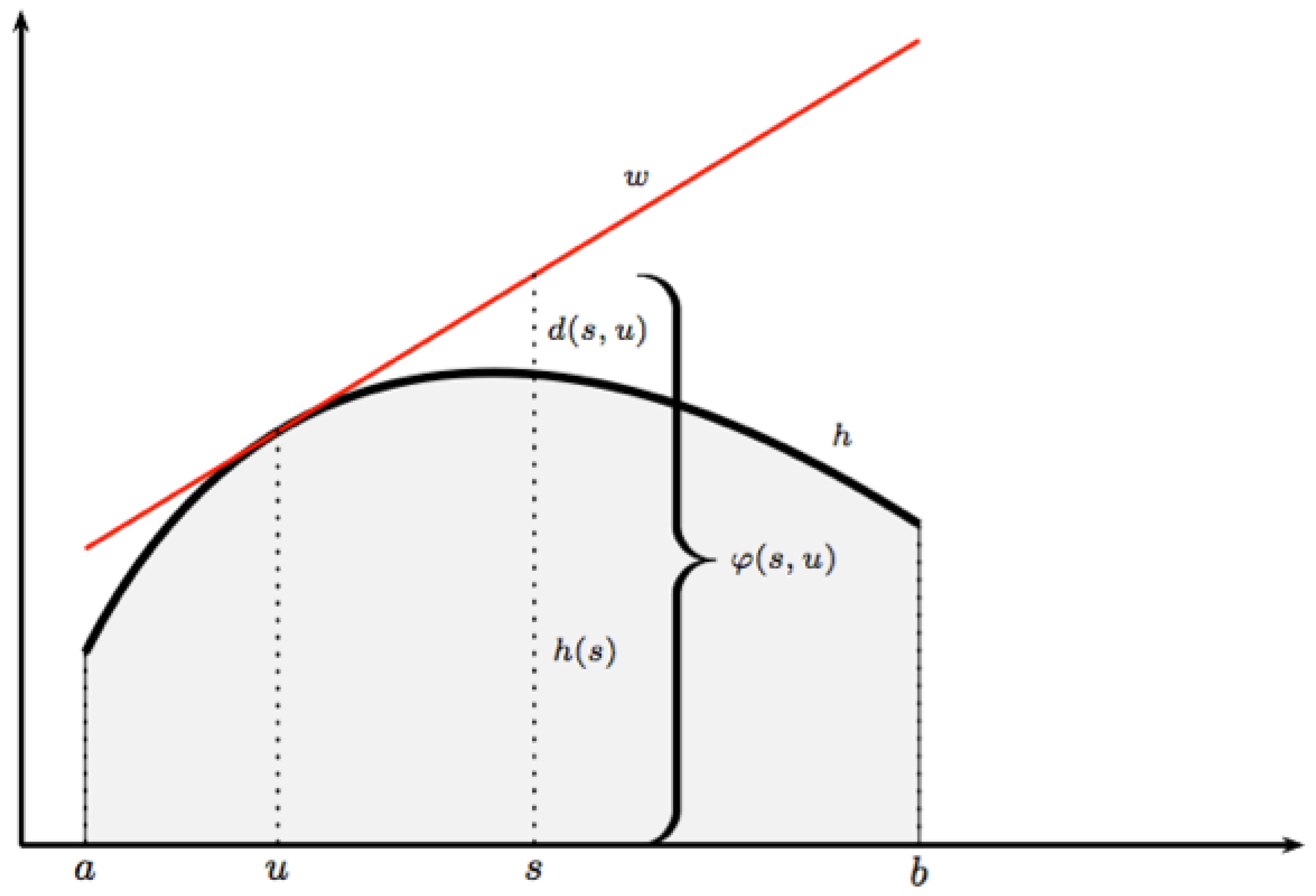
Given and a level , we define the level set and the sub level set by
i.e., as the set of states which are controlled by w, either at the level h or at the maximum level h. These sets are genuine preparations whenever they are non-empty. When w is the response of a state , is non-empty whenever . As level- and sub level sets for other functions will appear later on, cf., Section 2.14, we may for clarity refer to and to as, respectively, -level sets and -sub level sets.
The preparations in (26) we call primitive strict, respectively primitive slack preparations. A general strict, respectively a general slack preparation is a finite non-empty intersection of primitive strict, respectively primitive slack preparations. The genus of these preparations is the smallest number of primitive preparations (either strict or slack as the case may be) which can enter into the definition just given. Thus primitive preparations are of genus 1.
If are elements of and are real numbers, the sets
define strict, respectively slack preparations of genus at most n whenever they are non-empty. The set is the corona of whenever it is non-empty.
The preparations introduced above via the representation (27) are those we consider to be feasible and we formally refer to them as the feasible preparations. They provide the answer to the question about what can be known. They are the key ingredients in situations which Observer can be faced with. In any such situation a main problem concerns inference, an issue we shall take up in the next section.
Often, families of feasible preparations are of interest. Given , we denote by , respectively , the families which consist of all preparations , respectively , which can be obtained by varying .
Clearly, the feasible preparations can also be expressed by reference to the derived effort function rather than . We use the notation and for, respectively, the -level set and the -sub level set . If , and (note that for an expression such as , the nature of q determines if this is a - or a -level set). For finite sequences of elements of Y and of real numbers, the sets and are defined in the obvious manner as are the families of preparations , respectively .
The level sets may be used to define certain special belief instances or controls which will later, theoretically as well as for applications, play a significant role. Given is a certain preparation . Then, the core of consists of all belief instances y for which the effort is finite and independent of x as long as x is consistent. This notion, appropriately adjusted, also makes sense for the -domain. Notation and defining requirements are given as follows:
If , respectively , we also say that y, respectively w, is robust.
We shall refine the notions above in two ways. Firstly, for a family of preparations—such as a family of the form defined above—the core is defined as the intersection of the individual cores:
The second refinement we have in mind depends on on an auxiliary preparation , assumed to be a subset of the given preparation . For the -domain, a control is a -robust strategy for Observer if there exists a finite constant h, such that the following two conditions hold:
When we recover the original notion of robustness. The similar notion for belief instances is defined in the obvious way. Notation and defining relations for the corresponding adjustments of the notion of core are as follows:
From a formal point of view, it does not matter if we use -type sets or -type sets as the basis for the definition of feasible preparations. However, entering into more speculative interpretations, the -type sets which emphasize control seem preferable. Individual controls or a collection of such controls point to experiments which Observer may perform. An experimental setup identifies a certain preparation, and thus determines what is known to Observer. Determining all preparations which can arise in this way, we are led to the class of feasible preparations as defined above.
As to the nature of the various controls, we imagine that they are derived from description. To control a situation, you must be able to describe it, and with a description you have the key to control. We may imagine that, corresponding to a control w, Observer can realize a certain experimental setup consisting of various parts – measuring instruments and the like. In particular, there is a special handle which is used to fix the level of effort. If the level, perhaps best thought of as a kind of temperature, is fixed to be h, the states available to Nature are those in the appropriate feasible preparation. Several experiments can be carried out with the same equipment by adjusting the setting of the handle. If Observer wants to constrain the states by other means, he can add equipment corresponding to another control and choose a level for the experimental setup constructed based on . The result is a restriction of the available states to the intersection of the two preparations involved. If the preparation is and the actual state is not inside this preparation, you may imagine that the result is overheating and breakdown of the experimental setup! Thus you must keep the state inside the preparation and this may well be what requires an effort as specified by .
2.10. Inference via Games, Some Basic Concepts
For this section, is an effort-based information triple over and the derived triple over . Further, a preparation is given, conceived as the partial information “”. In practice, will be a feasible preparation, but we need not assume so for this section.
The process of inference concerns the identification of “sensible” states in —ideally only one such state, the inferred state. In many cases, this can be achieved by game theoretical methods involving a two-person zero-sum game. As it turns out, this will result in double inference where also either control instances or belief instances will be identified—ideally, only one such instance, the inferred control or the inferred belief instance as the case may be.
An inferred state, say , brings Observer as close as possible to the truth in a way specified by the method applied. The same may be said about an inferred belief instance—or you may find it more appropriate to view an inferred belief instance as a final representation of Observers subjective views and conviction. Turning to controls, an inferred control is conceived as an invitation to Observer to act, say regarding the setup of experiments and performance of subsequent observations. In this way, actions by Observer as dictated by an inferred control is conceived as that which is needed for Observer in order to justify the inference about truth. In short, double inference gives Observer information both about what can be inferred about truth and how.
Given , we shall study two closely related two-person zero-sum games, the control game , and the belief game , also referred to as the derived game. If need be, we may write and . The games have Nature and Observer as players and , respectively as objective function. Nature is understood to be a maximizer, Observer a minimizer. For both games, strategies for Nature involve the choice of a consistent state. Observer strategies for are controls from which every state in can be controlled. For , Observer strategies are belief instances from which every state in is visible, in other words, they are viewpoints of . Thus pairs of permissible strategies for the two games are either pairs with and (with the understanding that ) or pairs with and (with the understanding that ). In consistency with the discussion in Section 2.4, an observer strategy may be thought of as a strategy which is not “completely stupid” whatever the strategy of Nature, as long as that strategy is consistent. The choice of strategy for Observer may be a real choice, whereas, for Nature, it is often more appropriate to have a fictive choice in mind which reflects Observer’s speculations over what the truth could be.
A remark is in order regarding models where it is unnatural to work with controls and only belief is involved. Then the basis will be an effort-based information triple over and only one type of game, will be involved. Formally, this may be considered a derived game by artificially introducing , , by taking response to be the identity map and by taking to be identical with Thus the approach we shall take with a primary focus on the control games, based on objects for the -domain is, formally, the more general one.
Following standard philosophy of game theory, Observer should always be prepared for a choice by Nature which is least favourable to him. One can argue that in our setting anything else would mean that Observer would not have used all available information. The line of thought goes well with Jaynes thinking as collected in [9], though there you find no reference to game theory.
In order for our exposition to be self-contained and also because our games are slightly at variance with what is normally considered, we shall here give full details regarding definitions and proofs. As references to game theory and applications to the physical sciences, ref. [32,56,57] may be useful.
Let us introduce basic notions for the control game and then comment more briefly on the derived game. The two values of are, for Nature,
and, for Observer,
Note the slight deviation from usual practice in that w in the infimum in (36) varies over and not just over or some other set independent of x. Philosophically, one may argue that Nature does not know of the restriction to —this is something Observer has arranged—and hence cannot know of any restriction besides the natural one . As the infimum in (36) is nothing but the entropy , the value for Nature is the maximum entropy value, also referred to as the MaxEnt-value:
Problems on the determination of and associated strategies are classical problems known from information theory or statistical physics. If and , is an optimal strategy for Nature, also referred to as a MaxEnt-state or MaxEnt-strategy. The archetypal concrete problems of this nature are discussed in Section 3.7.
As to the value for Observer, we identify the supremum in (37) with the risk associated with the strategy w and denote it by :
The value for Observer then is the minimal risk of the game, also referred to as the MinRisk-value:
An optimal strategy for Observer is a control with , also referred to as a MinRisk-control or a MinRisk-strategy. Note the general validity of the minimax inequality:
Indeed, for arbitrary and arbitrary ,
and taking supremum over x and infimum over w, (41) follows. If (41) holds with equality and defines a finite quantity, the game is said to be in game theoretical equilibrium, or just in equilibrium, and the common value of and is the value of the game.
A further notion of equilibrium is attached to Nash’s name. It should, however, be said that for the relatively simple case here considered (two players, zero sum), the ideas we need originated with von Neumann, see [58,59] and, for a historical study, Kjeldsen [60]. A pair of permissible strategies is a Nash equilibrium pair for if, with these strategies, none of the players have an incentive to change strategy—provided the opponent does not do so either. This means, for Nature, that
and, for Observer, that
The inequalities (42) and (43) constitute a special case of the celebrated saddle-value inequalities of game theory. Note that, in our case, one of these inequalities (43), is automatic if is an adapted pair. This implies that and that as follows from the following trivial observation:
Proposition 1.
If and are permissible strategies for the two players in and if is adapted to , then and .
Proof.
By hypothesis, , and , hence , equivalent to the statement . ☐
Key notions and definitions for the belief game are quite parallel to what we have discussed for the control game. Briefly, the values of are (for Nature) and (for Observer) and notions of strategies and optimal strategies are defined in an obvious manner. We notice that the value for Nature in is , the same as the value for Nature in and that the notion of optimal strategies for Nature in the two games are equivalent notions. We use Ri as notation for risk in , i.e., for
Clearly, for any ,
Therefore, if and one of these belief instances is a viewpoint of , then so is the other and the associated risks are the same. The value for Observer in is
The game is in equilibrium if the two values of the game coincide and are finite. A pair of permissible strategies is a Nash equilibrium pair for if the two saddle-value inequalities hold:
Basic relationships between the values for the players in the belief game and the control game may be summarized as follows.
Proposition 2.
The values for Nature in and in coincide and are equal to the MaxEnt value . The corresponding values for Observer in the two games are , respectively . In general,
If response is surjective, equality holds in (49). Equality also holds if is in equilibrium. In that case also is in equilibrium and the values for the two games coincide: .
Proof.
The first statement regarding the values for Nature is trivial and also noted above. The inequality (49) follows by (45), which also implies that equality holds in case response is surjective. If is in equilibrium, apply the minimax inequality to , exploit equilibrium of as well as the inequality (49) and you find that
It follows that also is in equilibrium. Clearly, the values for the two games coincide. ☐
As it will turn out, in a great many cases of relevance for the applications, it is possible rather directly to identify optimal strategies for the players and to show that the games considered are in equilibrium. Furthermore, in many cases there is a natural relationship between the - and the -type games with the effect that, typically, there is a unique optimal strategy for Observer in and this strategy, a certain control, is adapted to any optimal strategy for Nature in the games and . Even more so, there is a tendency for the unique optimal control to be robust.
Results to support these claims will be taken up in Section 2.12. The results require that somehow you have good candidates for the hoped-for optimal strategies. For this, the indicated tendency towards robustness is a clue to how such candidates can actually be found in concrete cases of interest. In fact, a search for optimal objects via robustness is very efficient and more natural than the usual approach via the differential calculus as we shall also comment on in Section 2.12.
2.11. Refined Notions of Properness
The discussion to follow may appear unnecessary since normally, the standard notion of properness will apply. However, there are interesting cases where this is not so. Therefore, there is a need to look for suitable weaker notions which are still strong enough to have desirable consequences especially regarding properties of optimal strategies. As justification of the good sense in considering also the weaker notions of properness presented below we point to the general results of Section 2.12 and to the extended applicability of a a well-known construction due to Bregman, cf., Section 3.1 and Appendix A.
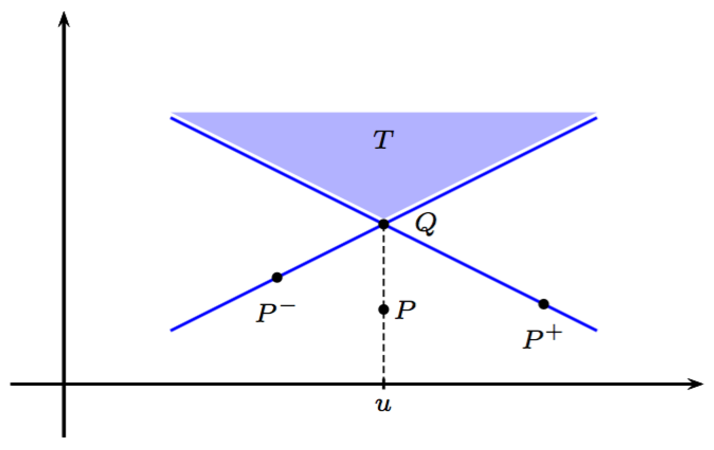
With assumptions as in Section 2.10, let us assume that is in equilibrium and, for simplicity, that there is a unique MaxEnt-state . Let us think of the system which Observer is studying as a physical system subject to the laws of statistical physics. Then Observer will expect that after some lead-in time, the system will stabilize and will represent the true state of the system. Observer aims at choosing a control which is optimal and at the same time adapted to Natures choice, . Unfortunately, Observer does not know which state this is among the consistent states. So Observer cannot just choose the control adapted to , but has to somehow choose some control of , say w.
At this point we introduce a built-in learning mechanism operating over time which may lead Observer in the right direction. The idea is illuminated by introducing an all-knowing being, Guru. Guru will not reveal the truth to Observer directly but may respond to specific questions. With this option, Observer may eventually end up by a choice of just the right control.
The three questions we shall consider all concern the entropy which Observer expects to be the MaxEnt-value. The questions are all related to the inequality
The questions put higher and higher demands on the chosen control w and are as follows:
- :
- :
- :
With Question , Observer wants to know if the effort he applies is minimal. Clearly, in view of the linking identity and the fundamental inequality—and as by the assumed equilibrium of —the question is equivalent to asking if . If the reply is negative, Observer knows that his choice cannot be optimal and he will then choose another control. But even with an affirmative answer, i.e., when , Observer may not be satisfied and may, therefore, continue the questioning. If the information triple is proper, an affirmative answer to will tell Observer that and he may be satisfied—even though it could still happen, as examples will show, that w is not optimal. Further questioning may thus only be needed if the information triple is not proper—or not known to be proper.
For the second question, , Observer is worried about his risk in case the state should somehow change. The question is equivalent to asking if . With a negative reply, Observer will dismiss the choice of w, if for no other reason, because w cannot be optimal then. If the reply is positive, w is optimal and one may wonder if Observer will still find any further checking necessary. The suggested third question reflects the ambition of Observer that he wants the control to be robust at the level .
Motivated by our considerations, we shall say that the information triple is , or -proper over if, with , we can conclude that w is adapted to from affirmative answers to, respectively, question , or . If we just talk about, say -properness, it is understood that the conditions hold with . If the entropy function is finite-valued, -properness is equivalent to (standard) properness.
Concerning questions being asked to Guru, one may wonder why Observer does not simply ask directly either if the chosen control is optimal or if it is adapted to the truth. In this connection, we remark that questions which can be asked to Guru must depend on the possibilities for Observer’s communication with the system. For a further discussion of this, one should replace Guru with some mathematically defined rules for this communication. Such rules may reflect the kind of experiments and associated measurements which Observer can perform on the system.
2.12. Inference via Games, Some Basic Results
We shall investigate the possibility to identify optimal strategies based on a suggestion of possible candidates. Moreover, when optimal strategies exist, we shall look at the ensuing consequences. This approach will involve problems which are easy to handle technically and yet, it may be argued that from an applied point of view the results obtained are of greater significance than theoretically more sophisticated results, such as those developed in Section 2.16. Several examples illustrating this point of view are listed in Section 3.
As in the previous section, an effort-based information triple over , the underlying triple, is given together with a preparation .
When we speak about an optimal state without any further specification it is understood that we have an optimal strategy for Nature in one of the games or in mind. As we observed in the previous section it does not matter which game we think of. Moreover, when we speak of an optimal belief instance, respectively an optimal control it is also clear what we have in mind, viz., an optimal strategy for Observer in , respectively in .
In our first result we investigate situations where, in addition to a requirement of equilibrium, there exist optimal strategies for both players.
Theorem 1 (Optimal strategies, basics).
(i): If is in equilibrium and both players have optimal strategies in this game, then also is in equilibrium and optimal strategies for both players in that game exist. Further, the values of the two games agree and, if are optimal strategies in , then are optimal strategies in (but there may be many other optimal strategies).
(ii): Now assume that is proper. Then, if is in equilibrium and both players have optimal strategies, say and , then , and . It follows that the optimal control is unique. Furthermore, also is in equilibrium and both players have optimal strategies. A belief instance is optimal in if and only if it has as response. If response is injective, each of the three optimal strategies associated with and —the optimal state , the optimal belief instance and the optimal control —are unique and .
Proof.
(i): Assume that is in equilibrium and that are optimal strategies for this game. A bit parallel to the reasoning in the proof of Proposition 2, we find that under the stated conditions
and the claimed assertions follow readily.
(ii): Now assume that is in equilibrium and that are optimal strategies for this game. By the defining relations (8) and (9), by the assumed equilibrium, by optimality of and of and by the definition (39) of risk, we find that
hence equality must hold throughout. Further, as , we conclude that , hence by properness that . Then, by Proposition 1, and .
Since above was an arbitrary optimal strategy for Nature and an arbitrary optimal strategy for Observer, and by the fact just established, we conclude that the optimal Observer strategy is unique and further, that all optimal strategies for Nature are response-equivalent, lie in and have the optimal control as response.
We leave it to the reader to establish the stated results for , say by noting that is equivalent with and that and by using the first facts established.
In case response is injective, the uniqueness assertions are easily established and the identity of and follows as these belief instances are response-equivalent. ☐
Some remarks are in order.
Remark 1.
Simple and very concrete “toy examples” over discrete sets—either finite or countably infinite—may be constructed to illuminate various assumptions and to investigate the limits of the conclusions. This involves matrix games which are easy to visualize. In this way one realizes that the games may be in equilibrium and yet there may be no optimal strategy for any of the players or there may be one or several optimal strategies for one of the players and none for the other. Three such examples for games in equilibrium and with an underlying proper information triple are indicated in Figure 1 where the rows are states and the columns controls (or belief instances). In case (a) there is a unique optimal control but no optimal state, in case (b) there is a unique optimal state but no optimal control and in case (c) all controls are optimal but there is no optimal state. It is also easy to construct an example where all states are optimal but no control is so.
Remark 2.
Regarding the necessity of injectivity of response in the last part of the theorem, note that if this condition does not hold, there may be strategies for Nature with the optimal control as response which are not optimal. Simple examples, say with “collapse of response”, i.e., with a singleton, will demonstrate that.
Remark 3.
Several remarks on the assumption of properness are in place. First note that we did not have to assume that response is surjective in order to prove that the optimal strategy in the second part of the theorem is in the range of this map. The assumed properness takes care of that. However, we need not assume that properness in its strongest form holds but may work with the weaker forms introduced in Section 2.11.
To make this more precise, first note that all assertions of the second part of Theorem 1 continue to hold if properness is replaced by -properness. This follows from the discussion in Section 2.11 by noting that from the relations in (51) one can conclude, not only that , but also that . In this way some of the concrete models discussed in Appendix A, can be handled—but not all.
We add, without going through the details, that if we assume that the weaker -properness holds in conjunction with an assumption of robustness, viz., that all controls which are adapted to an optimal state are robust, then uniqueness of a robust optimal control is secured. The robustness condition appears to be related to a requirement that response be defined “appropriately”. For the models of Appendix A this requires that special care is taken when defining response at boundary points of the state space.
In the sequel some results are proved under the assumption of -properness. This is, so we claim, a simple, worth while and natural extension over results proved only under an assumption of standard -properness. Even more general results involving also robustness as just indicated may well be possible. However, it seems that before that will make much sense, one should develop results and constructions going beyond what is indicated in Appendix A and in Corollary 6 further on.
Inspired by Theorem 1, a pair of permissible strategies is said to be a bi-optimal pair, if and if is the only optimal control. As follows from the theorem and from Remark 3, the required uniqueness property of is automatic under an assumption of -properness of the underlying information triple and further, must be adapted to .
If we have only given a state , we say that the state is bi-optimal if is a bi-optimal pair with adapted to .
Whereas it may be difficult to find optimal strategies, it is often easy to check if given candidates are in fact optimal:
Theorem 2.
[Identification] Under the assumptions of -properness, let be a state in with finite entropy and let be a control of .
Then a necessary and sufficient condition that the pair is bi-optimal is that it is a Nash equilibrium pair. If this is so, is adapted to .
Proof.
First note that (42) is equivalent with the requirement and that, because is known to hold (as ), (43) is equivalent with the requirement .
Thus, when (42) and (43) hold, we find, also invoking the minimax inequality, that
hence, recalling that , both and follow. By -properness, we then realize that is adapted to . Collecting facts established, we conclude that is a bi-optimal pair. This proves sufficiency.
The necessity and the last part of the theorem follow from Theorem 1 and the above noticed equivalent forms of the saddle-value inequalities. ☐
Elaborating slightly, we obtain the following corollary:
Corollary 1.
Under the assumption of -properness, if are permissible strategies for with , and with adapted to , then a necessary and sufficient condition that and are in equilibrium with as bi-optimal state is that , i.e., that
An important and trivial consequence of the existence of a bi-optimal state is the validity of the Pythagorean inequalities. Let be a bi-optimal state and its response. The direct Pythagorean inequality, or just the Pythagorean inequality, is the inequality , typically considered for . This is nothing but a trivial rewriting of (52). When it holds, and the inequality for an individual state is, therefore, a sharper form of the trivial inequality . The dual Pythagorean inequality is the inequality , typically considered for . When it holds, , and the inequality for an individual strategy is, therefore, a sharper form of the trivial inequality .
Theorem 3.
[Pythagorean inequalities] Under the assumption of -properness, if and are in equilibrium with as bi-optimal state then, with , the direct as well as the dual Pythagorean inequalities hold:
Proof.
As to (53), this follows from Corollary 1. Also (54) must hold since, for ,
☐
The Pythagorean flavour of (53) is more pronounced when one turns to models of updating, cf., Section 2.13 and Section 3.2.
Let us elaborate on the direct Pythagorean inequality. First, let us agree that a control w of is a Pythagorean control for if, for every ,
This notion will be used whether or not is in equilibrium and whether or not this game has optimal strategies. In particular, it applies in cases when no MaxEnt-state exists. Of course, the notion is only of interest if .
Translating to the Y-domain, we say that y is a Pythagorean belief instance for if and if, for every ,
Theorem 4.
Under the assumption of -properness, assume that a MaxEnt-state exists for the preparation and that . Then the following three conditions are equivalent:
- a Pythagorean control for exists;
- a Pythagorean belief instance for exists;
- The games and are in equilibrium and a bi-optimal state for these games exist.
If these conditions are fulfilled, the Pythagorean control, , is unique and identical to the optimal strategy for Observer in . Further, a belief instance, with is a Pythagorean belief instance if and only if it has as response.
Proof.
Assume that w is a Pythagorean control. Then, by (55), . Choose a MaxEnt-state . Then and (55) with implies that . As also holds, -properness shows that . Then, by Corollary 1, and are in equilibrium with as bi-optimal state. Appealing also to previous results, all statements of the theorem follow. ☐
The three results to follow are often useful in applications.
Theorem 5.
[Robustness theorem] Under the assumption of -properness, let be an adapted pair and assume that is robust for , say at the level h of robustness, and that is consistent. Then is in equilibrium with h as value and with as bi-optimal state. Furthermore, for any , the Pythagorean inequality holds with equality:
Similarly, if and are response-equivalent, if is robust for and if is consistent, then is in equilibrium with as bi-optimal state and, for ,
The equality (57) or (58) for is the Pythagorean equality, here in an abstract version. A more compact geometry flavored formulation of the first part of Theorem 5 in the direction of Corollary 1 runs as follows:
Corollary 2.
Under the assumption of -properness, if h is finite and , then and is in equilibrium with as bi-optimal state.
In case response is injective, the second part of Theorem 5 really only involves one element, , as the other element, , has to be identical to . The two essential conditions are one on as a strategy for Nature, viz., that it is consistent, and one on as a strategy for Observer, viz., that it is robust. There can only be one such element. If we drop the condition of consistency, there may be many more such elements. They form the previously defined core of .
For preparation families we find the following result:
Theorem 6.
Under the standard assumption on properness, consider a preparation family with . Let be a state, put and assume that . Further, put with for and assume that these constants are finite. Then and is in equilibrium and has as bi-optimal state. In particular, is the MaxEnt strategy for .
This follows directly from the involved definitions and from Theorem 5. The reader will easily establish an analogous result for the -domain.
The notions of robustness and core also make sense for games defined in terms of proper or just -proper utility-based information triples. If is such a triple, we simply apply the above definitions to the associated effort-based triple .
Theorem 2 points to a strategy which is often fruitful in the search for a MaxEnt-strategy, viz., first to determine the core of the given preparation and then to select that element (if any) in the core which is consistent. This route to determine MaxEnt strategies does not involve the infinitesimal calculus, in particular, it does not need the use of Lagrange multipliers. Researchers of statistical physics may claim that you need the Lagrange multipliers as they are of special physical significance, see e.g., Kuic [61]. In that connection, one will find that these quantities turn up anyhow and in a more natural way if you follow the approach via robustness, cf., [62].
The notion of robustness has not received much attention in a game theoretical setting. It is implicit in [26,63] and perhaps first formulated in [24]. Apparently, the existence of suitable robust strategies is a strong assumption. However, for typical models appearing in applications, the assumption is often fulfilled when optimal strategies exist. Results from [27] point in that direction.
Dual versions of the notions and results indicated above could be introduced, depending on (54) rather than on (53). However, it seems that the notions related to the direct Pythagorean inequality are the more useful ones.
For the result to follow we need an abstract version of Jeffrey’s divergence given, for two states and , by
Corollary 3.
[transitivity inequality] Assume that is a -proper information triple. If is in equilibrium with as a bi-optimal state, then, for every state and every belief instance , the inequality
holds. In particular, for every ,
Proof.
First note that also is in equilibrium with as bi-optimal state. Then, putting , (53) and (54) hold. Therefore, and as , for and ,
We refer to (60) as the transitivity inequality. It is a sharper version of the minimax inequality . It combines both Pythagorean inequalities and these are easily derived from it. If , the inequality holds with equality if and only if both Pythagorean inequalities (53) and (54) hold with equality.
As to the last part of Corollary 3, we note that if you put , then the bi-optimal state has Jeffrey divergence at most r from x.
For the final result of this section we shall work in the Y-domain based on the derived triple .
First we point to an extra property of bi-optimal states which follows from (53). In order to formulate this in a convenient way we need some definitions. A sequence of states converges in divergence to the state x, written , if . This requires that for all n (or for all n sufficiently large). If for all n, we say that is asymptotically optimal, more precisely asymptotically optimal for Nature in the game , if as . Finally, a state x (not necessarily in ) is a maximum entropy-attractor for with respect to convergence in divergence, more briefly, a -attractor for wrt D-convergence, if for every asymptotically optimal sequence .
We can now state a trivial corollary to Theorem 3 (transformed to the Y-domain):
Corollary 4.
Any bi-optimal state for a game in equilibrium, is a -attractor for wrt D-convergence.
We shall later demonstrate the existence of attractors in certain cases when the bi-optimal state may not exist. However, that will also involve a variant of the notion of attractor which relates to a different kind of convergence, convergence in Jensen-Shannon divergence, rather than convergence in divergence. The two concepts are identical in key cases as we shall later demonstrate (discussion after the proof of Theorem 11).
2.13. Games Based on Utility, Updating
In the previous section we investigated games related to an effort-based information triple. Similar notions and results apply when we start-out with a utility-based triple. Let us work in the Y-domain and base the first part of our discussion on a proper utility-based information triple over . Then, given a preparation , the associated game has Observer as maximizer and Nature as minimizer and the two values of the game are, for Nature, the minimax utility :
and, for Observer, the corresponding maximin value
For , the infimum occurring here is the guaranteed utility associated with the strategy y. We denote it . The maximin value (64) is also referred to as the maximal guaranteed utility. We denote it :
Notions and results, e.g., related to equilibrium, to optimal or bi-optimal states etc. are developed in an obvious manner, either by following Section 2.12 in parallel or by applying the results of Section 2.12 to the effort-based triple . The reader who wishes so will also be able to relax the assumption of properness to -properness.
Here, we limit the discussion to an elaboration of the important case of updating, cf., Section 2.8. For updating, according to Section 2.8, we do not need a full information triple. Therefore, for the remainder of the section we take as our basis a general divergence function D on , a preparation and a prior with on . The game associated with the utility-based information triple we denote . According to (63), the value for Nature in this game is , also denoted and referred to as the minimum divergence value or the MinDiv-value:
An optimal strategy for Nature is here called a D-projection of on . Consider an Observer strategy , i.e., a possible posterior. We use the same notation as in the general case, “Gtu” , to indicate Observer’s evaluation of the performance of the posterior. Incidentally, the letters can here be taken to stand for “guaranteed updating (gain)”. Thus
is the guaranteed updating gain associated with the choice of y as posterior, and
is Observer’s value of the game, the maximum guaranteed updating gain, or the MaxGtu-value of .
The basic results for the updating game may be summarized as follows:
Theorem 7.
Let D be a general divergence function on , a preparation and a belief instance with on . Consider the updating game .
If , then γ is in equilibrium with as bi-optimal state if and only if the Pythagorean inequality
holds for every . Moreover, if this condition is satisfied, is the D-projection of on . Furthermore, the dual Pythagorean inequality
holds for every .
The proof can be carried out by applying Corollary 1 and Theorem 3 to the effort function associated with the updating game considered, cf., (24). Details are left to the reader.
The concept of attractors also makes sense for updating games. Then the relevant notion is that of a relative attractor given , also referred to as the -attractor, which is defined as a state such that, for every sequence in with it holds that . In the situation covered by Theorem 7—assuming also that limit states for convergence in divergence are unique—the relative attractor exists and coincides with the bi-optimal state.
The Pythagorean inequality originated with Chentsov [64] and Csiszár [63] where updating in a probabilistic setting was considered. Further versions, still probabilistic in nature can be found in Csiszár [65] and in Csiszár and Matús [66]. In [67] these authors present a general abstract study, adapting a functional analytical approach building technically on meticulous exploitation of tools of convex analysis, partly developed by the authors. This source may also be consulted for information about the historical development and related works. As a work depending on a reversed Pythagorean inequality related to the triple (25), we mention Glonti et al. [68].
The reader should be aware that our notation deviates from what is most commonly found in the literature and promoted by Csiszár, mainly for classical Shannon Theory. Thus a relative attractor is mostly called a generalized I-projection (information projection). We have chosen to stick to the terminology with attractors, partly as their discussion is based on the primary results involving MaxEnt-analysis for which a terminology of projection is less natural.
2.14. Formulating Results with a Geometric Flavour
The results of Section 2.12 are formulated analytically. In this section we make a translation to results which have a certain geometric flavour. We shall work entirely in the Y-domain. No mention of controls or response will occur. This corresponds to a model with and where response is the identity map. Throughout the section results are based on a proper effort-based information triple .
In the previous sections, we had a fixed preparation in mind. Here, we shall also discuss to which extent you can change a preparation without changing the optimal strategy.
Sub Level sets of the form play a a key role. These sets appeared before as primitive feasible preparations. Here they have a different role and we prefer to use the bracket notation as above.
Proposition 3.
Let be a state with finite entropy . Then, given a preparation , the necessary and sufficient condition that the game is in equilibrium with as bi-optimal state is that is squeezed in between and , i.e., that . In particular, is the largest such preparation.
This follows directly from Theorem 2 and Corollary 1.
For a fixed preparation , we can express the two values of , and , in a geometrically flavoured way. This can be done whether or not the game is in equilibrium and the result can thus be used to check if the game is in fact in equilibrium. It is convenient to introduce some preparatory terminology.
Firstly, a subset of X is an entropy sub level set if it is a (non-empty) set of the form . The size of such a set is the smallest number a which can occur in this representation, clearly equal to the MaxEnt-value associated with the preparation . Given a preparation , the associated enveloping entropy sub level set is the smallest entropy sub level set containing .
Secondly, and quite analogously in view of (38) and (39), we introduce the size of the -sub level set as the smallest number a which can occur in this representation. And we define the enveloping -sub level set associated with to be the smallest -sub level set containing .
Proposition 4.
Consider the game associated with a preparation . Then:
- (i)
- The MaxEnt-value is the size of the enveloping entropy sub level set associated with ;
- (ii)
- For fixed , is the size of the enveloping -sub level set associated with .
- (iii)
- The MinRisk-value is the infimum over of the sizes of the enveloping -sub level sets associated with .
In view of (38)–(40), this is obvious. Some comments on the result are in order. In (i) it is understood that the size is infinite if no entropy sub level set exists which contains . A similar convention applies to (ii). Also note that the result gives rise to a simple geometrically flavoured proof of the minimax inequality (41) by noting that for each and each h, .
There are two families of sets involved in Proposition 4, the entropy sub level sets and the -sub level sets. As the proposition shows, both families give valuable information about the games we are interested in. From the second family alone, one can in fact obtain rather complete information. Indeed, if contains a given preparation for appropriately chosen y and a, the associated game is well behaved:
Proposition 5.
Given a preparation , a necessary and sufficient condition that is in equilibrium and has a bi-optimal state is that for some with and . When the condition is fulfilled, a is the value of the game and y the bi-optimal state.
The simple proof is left to the reader. It is the sufficiency which is most useful in practical applications.
The results above translate without difficulty to results about games associated with a utility-based information triple . For this, superlevel sets of the form as well as strict sub level sets of the form either or play an important role. The notion of size of these latter sets, those defined by strict inequality, is defined as the largest value of a which can occur in the representations given.
We shall consider the largest sets of the form , respectively , which are contained in the complement or, as we shall consistently prefer to say below, which are external to .
Either directly—or as corollaries to Propositions 3–5 applied to the effort-based triple —one derives the following results:
Proposition 6.
Let be a utility-based information triple and consider a state with . Then, for any preparation , the game is in equilibrium with as bi-optimal state if and only if . In particular, the largest such preparation is the superlevel set .
Proposition 7.
Let be a utility-based information triple and consider a preparation and the associated game . Then:
- (i)
- The value is the size of the largest strict sub level set which is external to .
- (ii)
- For fixed , is the size of the largest strict sub level set which is external to .
- (iii)
- The value , as the supremum of , is the supremum of all sizes of sets of the form with which are external to .
Proposition 8.
Let be a utility-based information triple and consider a preparation . Then a necessary and sufficient condition that is in equilibrium and has a bi-optimal state is that is external to for some with and . When the condition is fulfilled, a is the value of the game and y the bi-optimal state.
We also note that the minimax inequality follows from Proposition 7 by applying the fact that, generally, .
Let us look specifically at models of updating, cf., Section 2.13.
Given is a general divergence function D on and we consider preparations and priors for which on . The sets we shall focus on related to the games are of two types, which we associate with, respectively “balls” and “half-spaces”. Firstly, for , consider the open divergence ball with radius r and centre , defined as the -sub level set
In case for some state , we write this set as :
And, secondly, we consider sets—all referred to as half-spaces—of one of the following forms
Associated with the sets introduced we define certain “boundary sets” , respectively peripheries and hyper-spaces. Notation and definition for the former type of sets is given by
and for the latter type we use
When translating basic parts of Propositions 6–8 to the setting we are now considering, we find the following result:
Proposition 9.
Let D be a general divergence function on and consider a belief instance such that . Then the following results hold for the associated updating games with as prior:
- (i)
- For any , the largest preparation for which is in equilibrium with as bi-optimal state, hence with as the D-projection of on , is the half-space .
- (ii)
- For a fixed updating game , the MinDiv-value is the size of the largest strict divergence ball which is external to , and the maximal guaranteed updating gain is the supremum of a for which there exists such that the half-space is external to .
- (iii)
- An updating game is in equilibrium and has a bi-optimal state if and only if, for some , the half-space is external to . When this condition holds, y is the bi-optimal state, hence the D-projection of on .
For illustrations see cases (a) and (b) shown in the figure in Section 3.2.
2.15. Adding Convexity
It has been recognized since long that notions of convexity play an important role for basic properties of Shannon theory and for optimization theory in general, cf. in particular Boyd and Vandenberghe [54] which also has a bearing on many of the concrete problems treated later on. Deliberately, we have postponed the introduction of this element until this late moment, thereby demonstrating that a large number of concepts and results can be formulated quite abstractly and do not require convexity considerations. Also, it will become more clear exactly where convexity is needed.
We shall study results which can be obtained under added algebraic assumptions related to convexity considerations.
We assume that X is a convex set. The convex hull of a preparation is denoted . We assume that controllability is adapted to the convex structure in the sense that a control w controls a convex combination, say , if and only if w controls every with . It follows, that all control regions are convex. Also note that, for every convex combination , we conclude from that for all i with and hence, if we switch to the Y-domain, for every i with .
Regarding convex combinations, they are understood to be finite convex combination, often written as above without introducing any special notation for the relevant index set.
Properties of Concavity, convexity and affinity of real-valued functions f defined on X or on a convex subset of X are largely defined in the usual way. Thus, for concavity, the condition is that if is a convex combination of elements in the domain of definition of f, then . For convexity the inequality sign is turned around and for affinity it is replaced by equality. The notions make sense and will also be applied to extended real-valued functions provided they do not assume both values and . One comment has to be made, though. We only require that X is a convex set. However, X could be affine, i.e., combinations could be defined whenever the coefficients are arbitrary real numbers which sum up to 1. This will be the case for some models. We shall then point out if stated results hold for arbitrary affine combinations, not just for convex combinations.
The above definitions and concepts along with associated assumptions will always be understood to apply when, in the sequel, we work with a convex state space.
The basis in this section, except for the last part (Example 1 and Proposition 10), is a proper effort-based information triple over . The derived information triple over is denoted . When there is also given a preparation , the results developed continue to hold under -properness.
Emphasis will be on concavity, convexity or affinity for the w-marginals —either all of them or only those with a control in the range of the response function. Note that, say affinity for with w of the form for some amounts to the same as affinity of .
Basic properties of entropy and redundancy (hence also divergence) under added conditions about the marginals or are contained in the following result:
Theorem 8 (Deviation from affinity).
- (i)
- If the marginals with are concave, then, for every convex combination of elements in X,In particular, H is concave and if and this quantity is finite, then all with are response equivalent, in fact for these indices. If response is injective, the entropy function is strictly concave.
- (ii)
- (iii)
- If the marginals with are affine and if for a convex combination then, for every control w with ,
- (iv)
- If the marginals with are affine, if is a convex preparation with and if , then the restriction of to is convex and if for a convex combination of states in , then all with are response equivalent, in fact for these indices. If response is injective, the restriction of to is strictly convex.
Proof.
The result is a natural extension of (the main parts of) Theorem 1 of [55] and the proof is similar: For (i), apply linking to rewrite the right hand side, then upper bound the expression you get by the assumed concavity and you end with the upper bound . The results about concavity of H are easy consequences and property (ii) is proved similarly. For the basic assertion of (iii), add to both sides of (78), and use linking to rewrite the right hand side. Then apply the assumed affinity and the term appears to which you once more apply linking. Finally subtract from both sides. The assertions of (iv) are easy consequences. ☐
Several comments are in place. First, as a simple corollary to (i) of Theorem 8 we note the following:
Corollary 5.
Assume that the marginals with are concave and consider the game for a convex preparation . Then the set of optimal strategies for Nature in this game is convex and, in case response is injective and , there can be at most one optimal strategy for Nature.
Conditions of affinity will play a main role for many results to follow. Notions of affine equivalence applies in various contexts (-domain, Y-domain, effort-based or utility-based). Some examples will suffice: The effort functions and over are affinely equivalent if there exists a finite-valued affine function f on X such that, for , . If so, and are equivalent (). Moreover, two effort-based information triples and are affinely equivalent if they are equivalent and there exists a finite-valued affine function f on X such that, for , . Then of course, also .
A simple and practically important result which follows readily from affinity conditions exploits the notion of robustness in its weakened form introduced in Section 2.9, cf., (32) and (33). The result is an extension of Theorem 5.
Theorem 9.
Let X be a convex state space and let be a proper information triple over for which the marginals with are all affine. Let be a pair of permissible strategies for with adapted to . Assume that and that is -robust. Then is in equilibrium with as bi-optimal strategy.
Proof.
Then some comments on (79). In the terminology of [69], this is the compensation identity with the last term as compensation term. This term appears as a measure of deviation from affinity, both in relation to entropy, cf., (78), and in relation to redundancy (hence also to divergence), cf., (79). The significance of such terms is being more widely recognized. This applies in particular to the case of an even mixture , for which the term is called Jensen-Shannon divergence, briefly just JSD-divergence, between and . We shall use the notation
where a “bar” signals “midpoint of”, a notation to be used often in the sequel:
For even mixtures of two states, the compensation identity states that
which, for classical Shannon theory, is sometimes called the parallelogram identity. The identity makes sense for an arbitrary general divergence function but one should note the requirement of finiteness in (79), expressed somewhat indirectly via the entropy function. That some restriction is important will be seen from Example 1 below. When (82) holds, you may apply it with and with , and derive the identity
Previously, JSD-divergence has mainly been studied in the context of classical Shannon theory. For our more abstract theory, we have chosen to put emphasis on it, especially in the formulation of technical assumptions which are needed for the proofs of some basic results to follow. Note that JSD-divergence is everywhere defined on which D-divergence need not be. In the next section we take up a closer study of Jensen-Shannon divergence.
The purpose of the next result is to indicate that it is conceivable that for many concrete situations, a bi-optimal state will be robust, i.e., lie in the core of the preparation concerned. This result, in a more concrete set-up goes back to Csiszár, cf., [63]. It depends on the following notion: A state x is an algebraic inner point of (typically assumed convex) if, for every distinct from x, there exists such that x is a genuine convex combination of and .
Corollary 6.
Assume that is affine for all and let be a convex preparation. If is in equilibrium and has a bi-optimal state and if this state is algebraic inner in , then is robust for at the robustness level . In particular, .
Proof.
With assumptions as stated, consider any distinct from and determine such that is a genuine convex combination of x and , say . We find that . Similarly, . As the convex combination equals , we conclude that . As this holds for every , the result follows. ☐
An example is in place to illuminate the importance of the finiteness condition in relation to the compensation identity. We shall work in the Y-domain, for which the identity takes the following form:
The identity can be considered for more or less any bivariate function D on . As before let X be convex and assume that . We further assume that D is a general divergence function on . It may be that D is derived from an information triple over , but we do not assume so. In particular, no response function is involved.
In order to check if the compensation identity holds for D, you may check if the difference is well defined and independent of y. Or you may inspect more closely the expression for D. If this expression, apart from pure x-only dependent terms, only contains terms which, for fixed y, are linear terms in x, a suitable entropy can be identified and the compensation identity (84) will hold (when ). The procedure is demonstrated in the following example which, at the same time, also illustrates the role of the two assumptions made in part (iii) of Theorem 8 in order for (79) or (84) to hold.
Example 1.
Let be copies of the real line provided with the standard structure, let response be the identity map and let visibility be the diffuse relation. Further, let α be a positive parameter and consider the bivariate function D given by
Clearly, this is a genuine general divergence function.
If , (84) does not hold. Indeed, if you consider the mixture and as y take , then the left hand side of (84) equals whereas the right hand side equals . Thus, when , there is no information triple equivalent to for which (84) holds generally. So you cannot add a finite entropy function to and obtain an effort function with affine marginals.
If , the matter is quite different. Then and you can subtract to obtain a function with linear dependency on x for a given value of y. In other words, if you consider the triple equivalent to for which entropy is given by , all conditions of Theorem 8, (iii) are fulfilled, thus (84) must hold. Further material on this and similar examples can be found in Section 3.1.
For our last observation of this section we return to an updating triple as introduced in Section 2.8, cf. (22). Here, D is a general divergence and a prior. A certain preparation is also given and it is assumed that on . The triple is a genuine proper utility-based information triple over . It is still assumed that X is convex and that . The observation we want to point out is the following:
Lemma 1.
If, in addition to assumptions above, the compensation identity (84) holds for all convex combinations of states in and all , then all marginal functions of the utility function obtained by fixing an element are affine.
Proof.
Consider any and any convex combination of states in . As on , the sum is finite. By the compensation identity, so is the sum . For , we find that
This is the affinity relation sought. ☐
The significance of this result is that it will later allow us to apply results for the updating games under convexity assumptions, cf., Theorem 15.
2.16. Jensen-Shannon Divergence at Work
As in the previous section, X is a convex set. We assume now that . For the first part of the section we take as base a general divergence function D over . No preparation, effort function or entropy function will appear until later in the section. We work entirely in the Y-domain.
As is no surprise, not all results of information theory are constructive and in order to be able to handle situations where constructive methods are not available, we shall introduce topologically flavored notions and methods. Previously, as in [55], we introduced topology into the picture by referring to a “reference topology” which could be a topology with no very direct relation to the theory developed. Now we apply a different approach and insist that everything topological can be expressed in terms of quantities of direct interest for the theory dealt with. In fact, the previously defined Jensen-Shannon divergence (JSD), cf., (80), will now be the central quantity to work with. This notion of divergence is an everywhere defined, smoothed and symmetrized version of standard divergence. It may take the value . The following properties are obvious in view of the definition:
These properties hold for all . The same properties hold for any bivariate function on which is a function of some metric with a function defined on which vanishes at 0 and nowhere else. In several concrete cases, Jensen-Shannon divergence is of this type, in some central cases even in a very simple way as JSD will be a squared metric in the cases we have in mind. For research in this direction, we refer to Endres and Schindelin [70], Fuglede and Topsøe [71] and Briët and Harremoës [72]. The present study is a further indication of the significance of Jensen-Shannon divergence.
Jensen-Shannon divergence defines a natural sequential notion of convergence in X. To be precise, a sequence converges in Jensen-Shannon divergence to x and we write , if as . We shall only pay attention to convergence of ordinary sequences. Convergence in Jensen-Shannon divergence is also referred to as JSD-convergence.
A sequence is a JSD-Cauchy sequence if
We shall consider the following five properties:
We may use terminology such as JSD-convergence has unique limits or JSD convergence is complete, for example. Clearly C1, C2 and C4 hold generally. Completeness (C5) will be taken as an independent axiom. Adding two relatively innocent technical axioms, we shall also establish C3.
The axiom ASC of algebraic sequential continuity wrt JSD-convergence is the requirement that, for convex combinations and for a convex combination such that , and (hence also ) it holds that .
The axiom JSC of joint sequential lower semi-continuity of divergence is the requirement that, for and , it holds that, properly interpreted,
Regarding the proper interpretation of (96), we shall agree to define whenever . Thus the axiom implies that if the right hand side of (96) is finite, then must hold.
The significance of the properties C1-4 lies in a general result dueto Kisynski [73], see also Dudley [74], according to which these conditions ensure that the notion of convergence studied is topological, i.e., that there exists a topology on X for which sequential convergence coincides with the given notion of convergence. When this is so, there exists a unique strongest such topology, which we refer to as the associated topology. For this topology, a set is open if and only if any sequence which converges in the notion of convergence to a point in the set, eventually lies in the set. Note that, typically, there are many topologies for which sequential convergence coincides with a given notion of convergence. As a concrete example consider and note that the convergent sequences for the discrete topology (the eventually constant sequences) coincides with the class of convergent sequences for the strictly weaker topology specified by taking to be open if either or else with the uniform probability measure over (this is, essentially, “Appert space” of [75]).
We are now ready to prove the following result:
Theorem 10.
Under the added axioms ASC and JSC, the convergence properties C1-4 hold, hence JSD-convergence is topological and the associated topology is well defined. Further, JSD is a sequentially lower semi-continuous notion, i.e., for and , the following inequality holds:
Proof.
To establish (97), note that by axiom ASC the convergence is ensured. Then, by axiom JSC,
Similarly,
As the left hand side in (97) is the sum of the left hand sides of (98) and (99), and as the sum of the two right hand sides is dominated by the right hand side in (97), (97) must hold.
As to property C3, assume that and that . Then, by (97), and hence follows. By properness, and then follows. ☐
Under the discussion of properties (86)–(89) we indicated that often JSD is directly related to a metric in that a relation of the form
holds for some metric . In such cases it is mostly easy to identify the associated topology (without relying on any extra axioms). We leave it to the reader to prove the following simple result.
Proposition 10.
Assume that, for some metric ρ on X and some continuous and strictly increasing function f on with , Equation (100) holds for all . Then the associated topology for JSD-convergence exists and can be identified as the metric topology defined by ρ. Further, JSD is jointly lower semi-continuous. If the metric ρ is complete, so is JSD.
Under suitable conditions we now aim at establishing existence of optimal strategies for the players in the games . However, in certain important cases Nature does not have an optimal strategy. Instead, we aim at showing that rather generally replacements in the form of -attractors exist. We shall aim at attractors for JSD-convergence but, as it will turn out, under conditions stated, that will amount to the same thing as attractors for D-convergence. The result below, stated in rather full detail for reference purposes, is a main technical result of the present contribution.
Theorem 11.
Consider a convex state space X, let and let be a proper information triple over with affine marginals for all . Assume that the axioms ASC, JSC and the axiom of JSD-completeness which all relate to the divergence function D hold.
Then, for every convex preparation with , is in equilibrium and there exists a unique optimal strategy for Observer and a unique -attractor wrt JSD-convergence. Furthermore, and the direct as well as the dual Pythagorean inequalities hold, i.e., for and ,
Proof.
First we prove an auxiliary result, viz that if, for a sequence of states in and for a state , holds, then also must hold.
To see this, note that by assumptions made, we conclude from (iii) of Theorem 8 that, for all n, m and all ,
Applying this with , we see that is a JSD-Cauchy sequence. By completeness, there exists such that . By axiom JSD, , hence and follows.
Now, let be an asymptotically optimal sequence for . Then (i) of Theorem 8 applied to shows that
and we realize that is a JSD-Cauchy sequence. Therefore the sequence is JSD-convergent, say . If also is an asymptotically optimal sequence, there must, likewise, exist such that . As the alternating sequence is also asymptotically optimal, that sequence too JSD-converges, say with as limit state. By properties C2 and C3 we find that . This shows that there exists a unique -attractor wrt JSD-convergence. Let be this unique attractor.
Then we remark that if there exists an optimal strategy for Observer in , there can only be one such strategy and it must coincide with . To see this, note that if is optimal, , hence, for every , and hence is also an -attractor wrt convergence in D (cf., also Corollary 4). By the auxiliary fact established in the beginning of the proof, is also an -attractor wrt JSD-convergence, hence must coincide with as claimed.
Now fix an asymptotically optimal sequence, say . Then, for consider “suitable” convex combinations with and all positive (in fact, if the difference either vanishes or is larger than 1 and otherwise will do). Then
hence
Clearly, we can select the ’s such that this quantity converges to as . By axiom ASC, converges in JSD-divergence to and then, by axiom JSC, we conclude that . Since this holds for every consistent state x, , from which we conclude that is in equilibrium, that the direct Pythagorean inequality holds and that is an optimal strategy for Observer. As we have seen before, this strategy is unique.
As, for any ,
also the dual Pythagorean inequality holds. ☐
Several remarks concerning this theorem are in order.
Firstly, note that for the auxiliary result we started out to prove, we had to appeal (implicitly) to the finiteness condition in view of the condition in (iii) of Theorem 8. Alternatively, we could instead demand that the compensation identity holds unconditionally.
Then, in general, the D-notion and the JSD-notion of convergence may differ from each other (with D-convergence the stronger of the two). However, it follows from the theorem that under the conditions stated, it does not matter whether we define -attractors wrt D-convergence or wrt JSD-convergence. We may, therefore, simply talk about an -attractor, or even just an attractor, without specifying the mode of convergence we have in mind.
Further, it lies nearby to ask if also the inequality can be added to the conclusions in Theorem 11. If H is sequentially lower semi-continuous wrt D-convergence (or wrt JSD-convergence)—as will normally (always?) be the case—the inequality obviously holds. Assume now that this is the case. Then there are two possibilities why an attractor may fail to be an optimal strategy for Nature, either because or, more interestingly, because there is an entropy loss in that . In Harremoës and Topsøe [76], the authors speculate that the phenomena of entropy loss could be important in computational linguistics and provide a partial explanation behind Zipf’s law.
Following up on the remark above, we may investigate what can be accomplished if we work with a state which is known to be consistent and apply the same technique of proof as for Theorem 11. What we find is that in the presence of convexity (and with technical axioms added), the essential inequality is not needed in full strength. It suffices to assume one of the facts which flow from that inequality, viz., that . To be precise:
Theorem 12.
With assumptions as in Theorem 11, let be a convex preparation and a consistent state with finite entropy which is also a possible strategy for Observer, i.e., . Then the condition is not only necessary, but also sufficient for to hold, hence for to be in equilibrium with as bi-optimal state.
Proof.
Consider a state and apply (77) to a convex combination of the form . We find that from which we conclude that . By axiom JSD, and follows. As was arbitrary, the desired inequality follows. Apply Corollary 1 and the result follows. ☐
After these remarks let us turn to another key result:
Theorem 13.
Let be any preparation—convex or not—such that . Keeping the other assumptions of Theorem 11 as they are, the game is in equilibrium if and only if entropy is not increased by taking convex mixtures in the sense that
When (102) holds, and have the same unique optimal strategy for Observer and the same -attractor, for Nature and the two agree: .
Proof.
First remark that if (102) holds, and Theorem 11 applies. All claimed properties then follow easily from that result.
To prove necessity, note that quite generally,
In more detail, the condition is equivalent with , and, for each belief instance ,
This follows by standard assumptions made in the beginning of Section 2.15 according to which visibility is adapted to the convex structure and by affinity of the marginals (convexity would do). Then, if is in equilibrium, we can argue that
and (102) follows. ☐
As we saw, the result is essentially a corollary to Theorem 11. The proof above is modeled after the proof of a less abstract result in [55].
We have formulated results for the Y-domain which appear less involved. We leave it to the reader to formulate and prove versions of the two key theorems above for the -domain.
Translating Theorems 11 and 12 to a setting based on utility—this requires an obvious dual notion of attractors aiming at minimax utility rather than at maximin effort (i.e., maximal entropy)—one finds the following result:
Theorem 14.
Again with X a convex state space, let be a proper utility-based information triple with affine marginals for . Assume that the technical axioms ASC and JSC hold. Further assume that JSD-divergence is complete. Let be a convex preparation for which . Then:
- (i)
- Without further assumptions, the utility game is in equilibrium and there exists a unique optimal strategy for Observer and a unique -attractor . Furthermore, and the direct as well as the dual Pythagorean inequalities hold, i.e., for and ,
- (ii)
- In case is a consistent state with finite max-utility, i.e., for which , and the game is in equilibrium and has as bi-optimal state. In particular, the Pythagorean inequalityholds for every .
Let us collect the key results about updating games in one theorem:
Theorem 15.
Let X be convex, let be any preparation and let D be a general divergence on with for which the compensation identity holds. Assume that the technical axioms ASC and JSC hold and that JSD-divergence is complete. Consider a prior and assume that on and that . Then:
- (i)
- Without adding extra conditions, Observer has a unique optimal strategy, , in the game .
- (ii)
- Observer strategies for and for coincide, i.e., and, for every such strategy y, , hence
- (iii)
- If is convex, the game is in equilibrium and the -attractor exists. This attractor, say , is identical to the optimal Observer strategy from (i); it is the D-projection of on if and only if .
- (iv)
- The game is in equilibrium if and only if
Proof.
This may be proved by applying the key results of this section, also recalling Lemma 1. Details are left to the reader. ☐
Further properties of Jensen-Shannon divergence are worth investigating. This concerns in particular the notion of negative definiteness, cf., [71,72]. Some indications are in place. When the property holds, JSD is the square of a Hilbert metric in a natural sense (loc. cit.). Investigating this property, one will quickly realize that, modulo finiteness conditions on the entropy function (say ), JSD is negative definite if and only if the entropy function is midpoint-negative definite, i.e., for any finite sequence of states and any associated sequence of real numbers with , it holds that . If this property holds with a restriction on n we express the property by saying that H is -negative definite. Clearly, MP(2)-negative definiteness is equivalent to midpoint concavity of H. In the same way as we introduced the notion of -negative definiteness for H, we may introduce a notion of n-negative definiteness of JSD.
Whereas the results about embeddability in a Hilbert space are rather deep, if we just ask for the property to be a squared metric, the matter is much simpler:
Proposition 11.
Assume that JSD is everywhere finite. Then the following conditions are equivalent:
- JSD is the square of a metric;
- JSD is 3-negative definite;
- H is -negative definite
This result depends on the properties (86)–(89). The key argument is not specific to JSD. For the sake of good order, we provide a proof of the basic general result in Appendix D.
3. Examples, towards Applications
3.1. Primitive Triples and Generation by Integration
Natural building blocks for information triples will be defined. We shall here concentrate on a simple, important and easy-to-apply approach.
A possible expansion of the considerations in the present section is dealt with in the Appendix A. This is related to our introduction of weaker concepts of properness and will allow you to work more generally with non-smooth “generators” (see below). Desirable is also an introduction of an action space and of the notion of response. How this can be done is indicated in Appendix A. We have chosen not to deal with the possible refinements in the main text, partly to keep the exposition simple, partly as a few technical issues may still need a closer investigation.
Let I be a subinterval of with endpoints a and b (). Either none, one or both endpoints belong to I but neither nor are members of I. Provide I with its usual algebraic and topological structure. We take I as state space as well as belief reservoir. Thus . Visibility is normally taken to be the diffuse relation so that any state is visible from any belief instance. However, at times a more restricted notion of visibility is relevant, especially for or . Then
is a better choice.
We agree that in this section, visibility is either the discrete relation or else given by (110) in certain cases when is a left endpoint of I.
An effort-based information triple over is said to be primitive. The “primitivity” lies in the fact that the state space and belief reservoir appear to be as simple as one can think of—if you do not want to enter into discrete structures with a finite or countably infinite state space. We use lower case letters as in for such triples. Upper case letters will then occur for constructions via a process of summation or integration, starting with primitive triples.
We are especially interested in proper primitive triples. The conditions they must satisfy are as follows (linking, fundamental inequality, soundness and properness):
It is understood here and later on that such requirements are to hold for all (for (113)) or for all (for (111), (112) and (114)). From Section 2.15 we know that it is desirable for the effort function to have affine marginals . For this to be the case, there must exist functions on I, and say, such that
for . There is a simple way to generate a multitude of such information triples. The method is inspired by Bregman, [77], who used the construction for other purposes. Given is a Bregman generator h which is here understood to be a continuous, real-valued, strictly concave function on I which is sufficiently smooth on the interior of the interval, say continuously differentiable. We take this function as the entropy function, h. Defining effort and divergence by
the triple is indeed a proper primitive information triple with affine marginals, . Figure 2 illustrates what is involved.
It is also easy to illustrate geometrically what Jensen-Shannon divergence amounts to. Referring to Figure 3, we find that the Jensen-Shannon divergence between and , for primitive triples denoted by jsd is given by
It follows geometrically that
We also find that for a bounded interval I, JSD-convergence and D-divergence are equivalent concepts and that the associated topology is the standard topology on I.
The utility-based analogues of notions introduced are defined in an obvious manner (see also examples below). We shall use as generic notation for primitive utility-based triples.
As two examples of effort-based Bregman generated primitive triples, we point to the standard algebraic triple given by
over and to the standard logarithmic triple
over . Both triples are given in their effort-based versions. If need be, we refer to these triples as standard primitive effort-based triples.
The first triple is equivalent to a triple we met in Example 1. It leads to basic concepts of real Hilbert space theory by a natural process of summation or, more generally, integration. By a similar process, the second triple leads to basic concepts of Shannon information theory. Before elaborating on that, we shall generalize both examples by the introduction of a parameter q. In fact, we shall see that, modulo affine equivalence, both examples can be conceived as belonging to the same family of triples.
In order to modify the standard algebraic triple, it lies nearby to consider generators of the form
with and functions depending on a real parameter q. Let us agree to work mainly with as state space. Then q could in principle be any real parameter. For each fixed q, is either strictly concave—an effort-based Bregman generator—strictly convex—a utility-based Bregman generator—(or degenerate). Applications of (116) and (117) give the formulas
When is negative, is a genuine effort-based Bregman generator and the triple is a proper primitive effort-based information triple. When is positive, is strictly convex and the triple is a proper primitive utility-based information triple (which should then rather be denoted ). Thus, if you consider the triple you are certain to obtain a primitive triple, either effort-based or utility-based (or degenerate). It also follows from (126)–(128) that modulo affine equivalence, the triples you obtain from different choices of , and are scalarly equivalent. For some choices you may prefer to restrict the parameter so that only effort-based triples emerge, for others you may find it interesting to focus on triples where there is a smooth variation from effort-based to utility-based triples. In applications—purely speculative at the moment—this could reflect situations in economic or physical or chemical systems where e.g., a change from positive to negative rent or from exothermic to endothermic reaction can take place.
If you choose and , then equals
As you go from large to small values of q this primitive triple starts out as utility-based, then, for , becomes degenerate, after which it switches to the effort-based mode until, for , it again becomes degenerate, after which it switches back to the utility-based mode. For , the triple is the utility-based standard algebraic triple, the utility-based version of the triple given in (120)–(122). That triple is most naturally considered over with .
We can remove the “singularity” of the system at by blowing up the generator near . Let us choose and as follows:
Here, the constant represents an eventual overhead With choices as specified, we obtain the triples with
The Equation (131) gives you gross effort with net effort obtained by putting . Similarly, (132) is gross entropy and the same formula with gives you net entropy.
The family of triples (131)–(133) is well defined for all if we allow for an interpretation by continuity for . For the triple is degenerate, for it determines a proper primitive effort-based information triples. For continuity considerations show that is identical to the standard logarithmic triple given in (123)–(125) (assuming that the overhead is neglected, ).
The triples we have identified may all be conceived to be of the same structure as the standard logarithmic triple. What is meant by this, is that if we, following Tsallis [78], introduce the deformed logarithms, , defined by the formula
then the Formulas (131)–(133) may be expressed as follows in terms of the deformed logarithms:
These formulas are used for and (for negative q you do not obtain effort-based quantities). Note that if , then for . The formulas indicate that it is not so much the logarithmic function which is of importance but more so the function . This is no surprise to information theorists as the latter expression has a well known interpretation in terms of coding when , provided t represents a probability. No convincing interpretation of appears to be known for other values of q. For , (135)–(137) reduce to (123)–(125) pertaining to the standard logarithmic triple.
The family of triples (135)–(137), , is referred to as the family of deformed primitive triples—adding a qualifying “effort-based” if need be. The analogous utility-based primitive is the family of triples , i.e., for ,
Let us return to the process of integration hinted at in the beginning of the section. A substantial amount of concrete triples which illustrate the theory developed can be constructed by combining the Bregman construction with a process of integration.
Integration may be applied to any family of information triples and gives us new triples to work with. Note that by linearity of integration, the important property of affinity of marginals is preserved.
We comment mainly on integration of effort-based triples with a view towards applications in information theory and in statistical physics. Consider integration of one and the same primitive triple over with Bregman generator h. Partly for technical convenience we assume that h is non-negative. Then effort, entropy and divergence, will all be non-negative, also in the integrated version. Considering the intended applications, this is only natural.
Let T be a set provided with a Borel structure and with an associated measure . Let be the function space consisting of all measurable functions . Functions in X are identified if they agree -almost everywhere. Note that X is a convex cone. Consider the integrated triple
by which we express that the following equations hold:
As , H is well defined and for all and as is measurable and non-negative and measurable, cf., (117), D is well-defined by (144). By linking, also is well defined. Thus, is a well defined triple over . We leave it to the reader to verify that is a proper information triple. Moreover, if has affine marginals for all , then has affine marginals for all . The divergence functions which can be obtained in this way are Bregman divergences. Note that with this construction, the essential fundamental inequality even holds pointwise as . For this reason, when we discuss the integrated triple, we refer to (112) as the pointwise fundamental inequality.
Bregman divergence may be used to modify visibility by taking to consist of all pairs with .
For the standard logarithmic triple (123)–(125), one may construct discrete models, say over a finite or countably infinite alphabet T, by a process of summation related to the interval rather than the traditional choice . States will then be certain sequences , which may be conceived as intensity sequences consisting of point intensities rather than the usual probability sequences of point probabilities. As regularity conditions one could take sequences with bounded intensities or sequences for which the primitive entropy function h of (124) satisfies the requirement . For this to work technically, we realize the importance of the pointwise fundamental inequality for d of (125) and note that this requires the inclusion of the term in d. Thus one may suggest to replace classicalprobability spaces with certain intensity spaces.
Returning to the classical choice with discrete probability distributions over a discrete alphabet T, becomes discrete Kerridge inaccuracy, H classical Shannon entropy and D discrete Kullback-Leibler divergence. If we generalize to cover non-discrete settings, entropy can only be finite for distributions with countable support, whereas the generalization of divergence makes sense more generally. For instance, we may consider the generator on the entire half-line and for take an arbitrary measure space, provided with some measure . As state space we can then, as one possibility, take the set of measures absolutely continuous with respect to and with finite-valued Radon-Nikodym derivatives with respect to . For two such measures, say and we find that
This may be called generalized Kullback-Leibler divergence. It is the more natural divergence to consider. For one thing, the integrand is non-negative by the pointwise fundamental inequality. If we restrict attention to finite measures P and Q with the same total mass, this reduces to the standard expression . The standard expression also gives a divergence measure if the two measures are finite and and, moreover, the important compensation identity also holds in this case since the additional terms (stemming from in (125)) are integrable and affine.
Now consider extensions to cover also integration of the family . It is natural to consider these triples over with in order to ensure that . By integration we obtain the triples
defined over appropriate function spaces, typically representing probability distributions. For these triples are proper effort-based information triples. For you obtain degenerate triples. The quantity , is meaningful in discrete cases with T finite or countably infinite, and defines Tsallis entropy. For the continuous case, Tsallis entropy does not make much sense, but the divergence function does.
So far, we have discussed integration of primitive triples. This concerns a process where the original state space (the interval I) is changed to a new state space and then, an information triple over the new state space is constructed. A similar process applies if we start out with a family of proper information triples over the same state space X (formally, over or with structures as usual and, typically, ). Then we may consider the integrated triple
defined by
With suitable measurability conditions, is a well-defined proper information triple. Also, the standard restriction of affinity is preserved by this process. As a useful but trivial remark, we note that properness of the integrated triple only needs properness of for a set of positive -measure. An instance of this feature with T a two-element set was already discussed in Section 2.7.
The most obvious application of the process of integration probably is to integrate the utility-based standard algebraic triple , cf., (129). This triple is considered over with . Integrating over a measure space , you are led to take as state space the -space over . In standard notation, the integrated triple is given by
We collect in Section 3.2 comments on these classical concepts, seen in the light of the theory here developed.
Some comments on the generation of information triples by the method inspired by Bregman [77] are in order. The focus of Bregman’s method has often been on the divergence measures it generates. Before Bregman’s work one mainly studied f-divergences, introduced independently by Csiszár [79], Morimoto [80] and by Ali and Silvey [81]. We find that often, Bregman divergences occur more naturally and have more convincing interpretations.
As we have seen, the widely studied entropies bearing Tsallis’ name can be derived via a Bregman-type construction. In Section 3.6 we shall have a closer look at these entropies. They have received a good deal of attention, especially within statistical physics. Some comments on the origin of these measures of entropy are in place. Tsallis’ trend-setting paper [2] is from 1988 but, originally, the entropies go back to Havrda and Charvát [82], to Daróczy [83] and to Lindhard and Nielsen [84,85] who all, independently of each other, found the notion of interest. Characterizations via functional equations were derived in Aczél and Daróczy [86], see also the reference work [87] as well as [41]. Regarding the physical literature, there is a casual reference to Lindhard’s work in one of Jaynes’ papers [88]. However, only after the publication of Tsallis 1988-paper mathematicians and, especially, physicists took an interest in the “new” entropy measures. We refer to the database maintained by Tsallis with more than 2000 references. From the recent literature we only point to Naudts, ref. [89] who also emphasized the convenient approach via Bregman generators.
3.2. A Geometric Model
Let us return to the model given by (151)–(153) of Section 3.1. This is the utility-based information triple pertaining to the Hilbert space . The triple is proper and has affine marginals given y.
In this case, the linking identity (after rearrangement of terms) is identical to the cosine relation. Other well-known basic facts of inner-product spaces can be derived by combining the linear structure of such spaces with the basic properties of information triples. Thus, the identity you obtain from the compensation identity (79) applied to D is of central importance for classical least squares analysis (apparently, the identity has no special name in this setting—it goes back at least to Gauss).
Games directly associated with the information triple involve minimization of M over various preparations, in other terms, the search for elements closest to the origin subject to certain restrictions. Let us, instead comment on relative games, which are games depending on the specification of a preparation and a prior , cf., Section 2.8. If the preparation is convex and closed, the D-projection of on exists; it is the unique point in which is closest in norm to (though classical, the reader may appreciate to note that this existence result is derived with ease from the compensation identity and completeness of Hilbert space). As standard convexity- and continuity assumptions are also in place, Theorem 15 applies. It follows that the game is in equilibrium with the D-projection as bi-optimal state. The updating gain for this game is given by (21), i.e.,
In this case the Pythagorean inequality reduces to the classical inequality
valid for every .
Combining Proposition 9 and Theorem 15 we obtain rather complete information about the updating games, also for preparations which are not necessarily convex. For instance, Figure 4, case (a) illustrates a case with unique optimal strategies for both players and yet, the game is not in equilibrium. Case (b) illustrates a typical case with a game in equilibrium. For both figures, denotes the optimal strategy for Nature and the optimal strategy for Observer. Indicated on the figures you also find the largest strict divergence ball and the largest half-space which is external to . The two values of the game can then be determined from the figures, for Nature, respectively for Observer.
Lastly some words on the typical preparations you meet in practice. In consistency with the philosophy expressed in Section 2.9 these are the feasible preparations. The strict ones are affine subspaces and the slack ones are convex polyhedral subsets. We shall determine the core of families of strict preparations:
Proposition 12.
Consider a family of strict feasible preparations determined by finitely many points in X. The core of this family consists of all points in the affine subspace through generated by the vectors , i.e.,
Proof.
An individual member of is determined by considering all for which the values of have been fixed. Note that fixing these values is the same as fixing the inner products or, equivalently, the inner products . If is of the form given by (156), , then and we realize that this is independent of x if x is restricted to run over some preparation in . Then also is independent of x when x is so restricted. We conclude that . This proves the inclusion “⊇” of (156).
To prove the other inclusion, assume, as we may, that and that the forms an orthonormal system. Consider a point . Determine such that . By Theorem 5, is the bi-optimal state of . Let denote the common values of for . Then is the orthogonal projection of on , hence . This argument shows that the core is contained in the subspace generated by the . This is the result we want as we assumed that . ☐
In order to determine the projection of on a specific preparation , we simply intersect with . If you do this analytically, one may avoid trivial cases and assume that are linearly independent. In Figure 4, case (c) we have illustrated the situation in the simple case when .
3.3. Universal Coding and Prediction
In this and in the next two sections we present problems where randomization plays a role. It will be realized that apart from this, the discussion of the three problems treated, though different in nature, relies on the same type of considerations (Kuhn-Tucker type results).
We start by discussing a problem of universal coding and prediction.
Let be a discrete finite set, the common alphabet and consider languages whose written representation use letters from . Let be a finite set of such languages, referred to as the selection, e.g., the selection could be English, German and French. Assume that for each individual language from we know the distribution of single letters in a typical text from that language, and let us identify a language with the corresponding distribution over . In this way, the selection is identified with a certain finite subset of , the set of all distributions over .
When we observe letters from generated by a typical text from just one of the languages, say with associated single-letter distribution , information theory tells us how to encode letters from in strings of letters from a reference alphabet, say the binary alphabet consisting of the two elements 0 and 1, so as to minimize the expected length of the encoded binary strings. The encoded string corresponding to the letter , will then have a length which is given roughly as
with log denoting binary logarithms. This choice ensures that the average code length
is minimal.
The precise sense in which (157)—even with exact equality—is the undisputed right choice will not be discussed here. It is a cornerstone of information theory for which you may consult standard text books on information theory such as [90] or an introductory text such as Topsøe [91]. Note that (157) with equality implies that (Kraft’s equality).
Let us change to a more theoretical concept of encoding by idealization, forgetting that the length of a binary sequence is a natural number and by a change to natural units rather than binary units. This leads us to redefine a code over to be a map such that
i.e., such that Kraft’s equality with natural units holds. Denote by the set of all such codes. The requirement (159) amounts to the requirement that the correspondence given by
is a one-to-one correspondence between and . We also express (160) by saying that is adapted to P and we write . As is easily seen, either directly or referring to previous material from Section 3.1, is the unique code for which the average code length is minimal.
With this property in mind, we define the redundancy of a pair as the quantity
From our discussion we know—in a theoretical idealized way at least—how to encode letters from if we want to process letters from a text source generated by a single language in an optimal manner. We shall investigate what can be done if we receive text from an unknown language, except that we know that the language is one from the given selection.
We agree to call a code universal for the language selection if the risk, here defined as
is minimal. The associated distribution under the correspondence is then said to be a universal predictor. Note that the risk is associated with the information triple and that a universal code is the same as an optimal strategy for Observer in the game associated with this triple. Clearly, the game in question is not in equilibrium, hence equilibrium type results as developed previously are not of much use. Instead it turns out that a very direct approach will lead to an identification of universal objects.
Theorem 16.
Let with adapted to . Assume further that for some finite constant R,
and that can be written as a convex combination of a set of distributions in for which equality holds in (163). Then is the unique universal code and the unique universal predictor.
Proof.
Clearly, .
Then consider any code different from . Write as a convex combination of distributions in all of which satisfy the relation . Then the compensation identity tells us that
Thus, as is proper, . As this holds for all , the result follows. ☐
Note the essential point that satisfies the compensation identity. That this is so follows either by direct calculation or, more systematically, by applying (iii) of Theorem 8 to the triple you obtain by adding entropy to . For the derived domain you then work with the typical Shannon triple, listed explicitly in (185)–(187). So, after all, the information triples are also useful for the above problem.
It can be shown that the result always applies in the sense that the unique optimal code and the unique optimal predictor exist and that they satisfy the conditions stated in the theorem. Note that the representation of the optimal predictor as given in the theorem may not be unique.
3.4. Sylvester’s Problem from Location Theory
As starting point we take a simple Y-domain model with , a convex set. For visibility we take the diffuse relation . Given is a finite-valued general divergence function over for which the compensation identity (79) holds.
As a concrete example, one may have in mind, take that of a Euclidean space X provided with norm-squared distance, . Moreover, as the motivating problem, consider Sylvester’s problem, to determine the point with the least maximal distance to a given finite set of points in X, cf., [92] or the monograph [93]. For the original problem, X was the Euclidean plane. However, the problem makes good sense in the general setting with X any convex set provided with a suitable replacement for classical squared distance.
The problem is a minimax problem and may formally be conceived as related to the special proper information triple . Indeed, the problem is to find optimal Observer strategies for the associated game and to calculate Observer’s value of the game, the MinRisk-value . However, this game is rather trivial as Natures value in the game is 0. Thus no equilibrium-type results are available.
To find a remedy, we apply a process of randomization. For that, we no longer consider X as the state space but take the convex space of molecular probability measures as a new state space. An element is represented as a family of non-negative numbers such that and such that the support of , i.e., the set , is finite.
The new model we shall construct is conceived as a -type model. As state space we take . Just as X, this is a convex set. For formal reasons—so that the modeling fits the general abstract theory—we may also take as belief reservoir, though we will have no need really to consider belief instances. Instead, control will be in the focus, and for the set of control instances we shall take . Once more for formal reasons, we consider the barycentric map which maps an (artificial) belief instance into its barycenter as response. This map will play an important role for the modeling. Let the map be with and barycenter of given by
The good sense in considering elements of X as controls is the idea from location theory, that from a point in X, conceived as a location, you should try to control the given points in the set as best you can.
With these preparations, we may consider the triple over given by
For , denote by the set of which are supported by , i.e., . By we denote the game corresponding to the triple with as preparation. A basic fact which contributes to the significance of games of this type is that, as easily seen, risk does not increase when you replace the game with , in particular, with self-explanatory notation,
This fact relies on the affinity of the marginals of for fixed y.
Theorem 17.
The triple over is a proper information triple over and the triple has affine marginals.
Let be a subset of X and consider the game . Consider a pair of strategies in the game with adapted to , i.e., . Then if, for some constant R,
is the unique optimal strategy for Observer in as well as in . Further, and is a bi-optimal strategy for .
Proof.
With preparations done, the first part is trivial, and the second is also so, obtainable as an application of Corollary 1. ☐
Note that the linking identity is just another way of formulating the compensation identity and that the entropy function is the compensation term in that identity.
With Theorem 17 we have a solution to Sylvester’s problem for an abstract model provided you can somehow point to a possible solution. It can be shown, modulo technical assumptions to ensure existence of optimal strategies, that the sought optimal Observer strategy must be of the form as stated in the theorem.
3.5. Capacity Problems, an Indication
Problems concerning capacity are among the most well known problems from information theory. They concern the determination of capacity defined as maximal information transmission rate under various conditions and on the associated optimal ways of coding. We shall only define one of the basic concepts and derive a key relation and leave it to the reader to consult the literature for more concrete results.
We first elaborate on the information triple given in the previous section by (165)–(167). The entropy function of that triple we may think of as related to information transmission rate of information theory (then also related to the notion of mutual information which is, however, not investigated further in the present study). This refers to the map as a map from an input letter to an output letter. Then an element represents a distribution over the input letters, a source, and response tells you what is happening on the output side. It is important to study how the rate behaves under mixtures. Thus we have a need to study elements in . The result one needs exploits the flexibility of the modeling, especially related to Theorem 8.
First, define information transmission rate related to simply as
We wish to emphasize the following result:
Lemma 2.
With the setting as above, consider any and put . Then, for every ,
Proof.
If you write in place of I, this follows from the identity (77) of Theorem 8 with in place of H. ☐
With the technical lemma in place, a study of abstract models of information transmission systems runs smoothly and you can derive operational necessary and sufficient conditions for the requirements of optimal strategies. On Natures side, an optimal strategy is an input distribution for which the transmission rate reaches the maximum, the capacity of the system. The result is a Kuhn-Tucker type result, well known from general convexity theory and from Information theory, and much resembles the results of the previous two sections. We refer to Topsøe [94] for an exposition of a result which exploits the lemma just proved.
3.6. Tsallis Worlds
Recall the introduction in Section 3.1 of the family of Tsallis entropies. In this section we present arguments which may help to appreciate the significance of these measures of entropy.
The main result, Theorem 18 was presented in a different form in [36] and, less formally, in [35]. Here we present detailed proofs which were not provided in these sources.
The introduction in Section 3.1 of the Bregman generators and thereby, via a process of integration, of Tsallis entropy, cf., (146), does not in itself constitute an acceptable interpretation. Via coding considerations, the significance of the Bregman generator , leading to the notion of Shannon entropy is well understood. Despite some attempts to extend this to more general entropy measures, cf., [95,96,97], a general approach via coding has not yet been fully convincing. In [98] you find a previous attempt of the author centred on a certain property of factorization.
The results presented here indicate that possibly, a convincing and generally acceptable physical justification of Tsallis entropy can be provided by involving deformation between the physical system studied and the physicist. Previous endeavours to find physical justification for Tsallis entropy are discussed in detail in Tsallis, [99]. We share the view that though the “Tsallis-q” can be viewed just as a parameter introduced simply to fit data, this is not satisfactory and operational justification is needed. Deformation as here emphasized in combination with a notion of description may offer a common ground on the way to more insight.
To set the scene for our study, introduce the alphabet , a discrete set of basic events which are identified by an index, typically denoted by i. Sensible indexing is often of importance and depends on the concrete physical application. The semiotic assignment of indices shall facilitate technical handling and catalyze semantic awareness. As we have no concrete application in mind, no extra structure is introduced which could justify a specific choice of indices.
The state space X is taken to be identical to the belief reservoir Y and, for simplicity, equal to , the set of probability distributions over (you could have worked, instead and more generally, with sets involving intensity as suggested in Section 3.1). Generically, will denote a state and a belief instance. Thus x and y are characterized by their point probabilities. As , the set of certain belief instances, we take the set of deterministic distributions over . Visibility shall mean that x is absolutely continuous wrt y. Thus consists of all pairs with , with @supp@ denoting support. We shall not need a control space or a response function.
A knowledge instance will be a family over of real numbers, not necessarily a probability distribution. The interpretation of is as the intensity with which the basic event indexed by i is presented to Observer. For this reason, z is referred to as the intensity function. The individual elements are the local intensities.
The deformation between x, y and z is given by a deformation , cf., Section 2.5. We assume that acts locally, i.e., that there exists a real-valued function , the local deformation, defined on such that, when , then for all . The world defined in this way by a local deformation is denoted or, if need be, . From now on, when we talk about a “deformation”, we have a local deformation in mind.
Regarding regularity conditions, we assume that is finite on , continuous on and continuously differentiable on . The deformation is weakly consistent if whenever and . If you can even conclude that is a probability distribution, is strongly consistent. The deformation is sound if for every .
For , the algebraic deformation is given on by
These deformations are all sound and weakly consistent and, for , even strongly consistent. The corresponding worlds are denoted . The notation is consistent with the notation introduced in Section 2.5. The significance of the algebraic deformations is derived from the following result.
Lemma 3.
Assume that the alphabet is countably infinite. Then only the algebraic deformations are weakly consistent.
Proof.
Let be weakly consistent and put . Consider a deterministic distribution over and apply weak consistency with to find that . Thus, if x and y both have support in a subset , you can neglect contributions stemming from with and conclude consistency over , i.e., that . By weak consistency (in the extended form just established), for all , in particular, . Consider and for , apply weak consistency and conclude that . Then, for , consider vectors of the form . By weak consistency and previous findings, conclude that for all rational . By continuity, this formula holds for all . Quite analogously, for all . Finally, follows by weak consistency applied to . ☐
In particular, if is infinite then, automatically, a weakly consistent deformation is sound. In fact, all concrete deformations we shall deal with will be sound.
Instead of searching only for a suitable entropy function for the world , we find it more rewarding to search for a suitable full information triple for this world. Let us analyze what such a triple, say , could be. A natural demand is that and D should all act locally. Therefore, according to Section 3.1 what we are really searching for is a primitive information triple over , cf., (110), such that is obtained from this triple by integration over equipped with counting measure. In particular, the requirements (111)–(114) must be satisfied. Obvious names for the sought functions and d are, respectively, local effort, local entropy and local divergence.
Let us suggest a suitable form of local effort. It will depend on the notion of a descriptor, defined as any continuous, strictly decreasing function on which is finite-valued and continuously differentiable on , vanishes at and satisfies the condition that
The value is conceived as the effort you have to allocate to any basic event in which you have a belief expressed by u. The condition reflects the fact that if you feel certain that a basic event will occur, there is no reason why you should allocate any effort at all to that event. Also, it is to be expected that events you do not have much belief in are more difficult to describe than those you believe in with a higher degree of confidence. Therefore, we may just as well assume from the outset that is decreasing. The norming requirement (174) will enable comparisons of effort, entropy and divergence across different descriptors or even different worlds. The unit defined implicitly by (174) is the natural information unit, the “nat”.
An important class of descriptors is the class given on by
With access to a descriptor you may suggest to assign the effort to an event with belief instance u, but you should multiply this effort with the intensity with which the event is presented to you. This gives the suggestion for local effort. Then local divergence should be the function . However, this is not going to work as the fundamental inequality (112) is bound to fail (consider with u close to 1). Fortunately, insight gained in Section 3.1 indicates how one may modify the suggestion in order to have a chance that the fundamental inequality could hold, viz., by adding an overhead term. Therefore, given a descriptor, we now suggest to define the local functions as follows:
One may study modifications with more general overhead terms, but we shall not do so. The important thing is to realize that something has to be done. Moreover, inspired by the fact that for the important cases with descriptors of the form , adding a simple linear overhead as suggested above works. This is stated explicitly in Corollary 7 below.
Lemma 4.
Let π be a deformation and κ a descriptor. Assume that given by (178) is a genuine primitive divergence function, i.e., that (112) (the pointwise fundamental inequality) and (114) (pointwise properness) hold. Then obtained by integration of the local quantities given in (176)–(178) over is a proper information triple over .
The proof follows directly from the discussion in Section 3.1.
Note that for sound deformations, the measures of entropy constructed this way only depend on the descriptor, not on the deformation.
Also note that the quantities defined really give gross effort and gross entropy. In particular, minimal entropy is not 0 as usual, but 1. This may appear odd but, on the other hand, the way to these quantities was very natural and one may ask if it is not advantageous in many situations to incorporate an overhead. Moreover, why not use the overhead to fix the unit of effort?
We also remark that if we allow incomplete probability measures Q as belief instances, then this change of the space will not change the conclusion above. However, sticking to probability measures also for belief instances, we may subtract the number 1 from gross effort and from gross entropy and obtain the more familiar net-quantities.
Corollary 7.
For the deformation and the descriptor satisfy the conditions of Lemma 4. Accordingly, the information triple generated by integration over is a proper information triple. Furthermore, the effort function has affine marginals.
The obtained effort- and entropy functions are gross-quantities. The corresponding net-quantities give the information triple in (146) of Section 3.1. In particular, is standard Tsallis entropy with q as parameter.
The simple checking is left to the reader.
We turn to problems of another nature, viz., if, given a deformation, one can find an appropriate descriptor such that the generated global description effort is proper.
Lemma 5.
Assume that the alphabet has at least three elements. Let π be a sound deformation and denote by χ the function on defined by
Under the assumption that χ is bounded in the vicinity of , there can only exist one descriptor κ such that the net-effort function generated by π and κ, i.e., the function Φ given by
is a proper effort function over . Indeed, κ must be the unique solution in to the differential equation
for which .
Proof.
Assume that exists with proper. For put
Consider a, for the time, fixed probability vector with positive point probabilities. Then the function F given by
on assumes its minimal value at the interior point when restricted to probability distributions. As standard regularity conditions are fulfilled, there exists a Lagrange multiplier such that, for ,
when . This shows that .
Using this with for a value of x in , we conclude that f is constant on . Then consider a value and the probability vector and conclude from the first part of the proof that . As , we conclude that . Thus f is constant on . By letting in (181) and appealing to the technical boundedness assumption, we conclude that the value of the constant is . ☐
Note the use in the above proof of Lagrange multipliers in the study of properties that hold under the realization of an extremum. This is quite different from the usage we have opted against where the technique is used as a tool to verify that an extremum has been found. In the latter case, we claim that, typically, more adequate intrinsic methods apply.
We can now formulate one of the main results:
Theorem 18.
Assume that the alphabet has at least three elements.
- (i)
- If , there is no descriptor which, together with , generates a proper effort function.
- (ii)
- If there exists a unique descriptor, defined by (175) which, together with generates a proper effort function. The generated information triple is proper.
Proof.
By Lemma 5 we see that given by (175) is the only descriptor which, together with , could possibly generate a proper effort function. That it does so for , follows by Lemma 4. For , this is not the case as the reader can verify by considering atomic situations with and and letting tend to 0. ☐
We may add that for the case of a black hole, , the descriptor is given by and, using for “number of elements in ⋯” , the generated information triple is given by
for all . Note that if terms of the form were to be interpreted by continuity, the resulting triple would be discrete.
We have noted that the descriptor is uniquely determined from the deformation. Therefore, in principle, only the deformation needs to be known. Examples will show that different deformations may well determine the same descriptor. For instance, deformation defined as a geometric average rather than an arithmetic average as in the definition of will lead to the same descriptor. Thus, knowing only the descriptor, you cannot know which world you operate in, in particular, you cannot determine divergence or description effort. But you can determine the entropy function. This emphasizes again the general thesis, that entropy should never be considered alone.
Finally a comment on the descriptors . A focus on their inverses is also in order. They may be interpreted as probability checkers: Indeed, if, in a Tsallis world with parameter q, you have access to a nats and ask how complex an event this will allow you to describe, the appropriate answer is “you can describe any event with a probability as low as ”. Thus, when , however large your resources to nats are, there are events so complex that you cannot describe them, whereas, if you can describe any event if you have access to K nats if only K is sufficiently large ().
3.7. Maximum Entropy Problems of Classical Shannon Theory
Terminology and results as developed in Section 2 are evidently inspired by maximum entropy problems of classical information theory. The classical problems concern inference of probability distributions over some finite or countably infinite alphabet , typically with preparations given in terms of certain constraints, often interpreted as “moment constraints” related to random variables of interest. Such preparations will, modulo technical conditions, be feasible in the sense as defined in Section 2.9. Examples are numerous, from information theory proper, from statistics, from statistical physics or elsewhere. The variety of possibilities may be grasped from the collection of examples in Kapur’s monograph [100]. The abstract results developed in Section 2 can favorably be applied to all such examples. This then has a unifying effect. However, for many concrete examples, it may involve a considerable amount of effort actually to verify the requirements needed for the abstract results to apply. This may involve the verification of Nash’s inequality (52) or the determination of the core of models under study, cf., Theorems 5 and 6. No detailed calculations for specific examples will be carried out here.
A very large number of researchers have worked with these problems. The related publications of the present author comprises [26,101]. We shall focus on applications of the general theory from Section 2.
The basic model we shall discuss is the same as in Section 3.6 based on a finite or countably infinite alphabet . Note that, in principle, discrete alphabets with more than enumerably many elements could be allowed. However, that would contradict the sensible requirement (3).
The relevant information triple is the proper information triple composed of Kerridge inaccuracy, Shannon entropy and Kullback-Leibler divergence:
We shall also work with the action space introduced in Section 3.3 and as response we take the bijection from Y to given, for , by
Controllability is the relation for which control means that whenever . The information triple to work with in the -domain is with entropy as above and with
The triples and are genuine proper information triples with affine marginals. Thus all parts of the abstract results developed are available and ready to apply. However, we limit the discussion by focusing only on the role of the feasible preparations, leaving elaborations in concrete examples to those interested.
Thinking of states P as determining the distribution of a random element over , it is often desirable to consider preparations corresponding to the prescription of one or more mean values of . A typical preparation consists of all such that
with c a given constant and a given function on . This is a strict feasible preparation if and only if the partition function (a special Dirichlet series),
has a finite abscissa of convergence, i.e., converges for some finite constant , cf., [26] (or monographs on Dirichlet series). However, for the most important part, having concrete applications in mind, viz., the “if”-part, this is clear. Indeed, if the condition is fulfilled, there exist constants and such that the function given for by
defines a code. Then for some constant k, hence it is a strict feasible preparation of genus 1. It is a member of the preparation family . Consider, for any with , the code given for by
Then this code is a member of as is easily seen. In fact all members of the core are of this form (this fact can be proved as a kind of exercise in linear algebra, but more elegant proofs using the structure of the problem should be possible). If we can adjust the parameter such that the corresponding distribution given by
is a member of the original preparation , this must be the maximum entropy distribution of , as follows from Theorem 6, translated to the -domain.
Schematically then: In searching for the MaxEnt distribution of a given preparation, first identify the preparation as a feasible preparation (of genus 1 or higher), then calculate if possible the appropriate partition function and finally adjust parameters to fit the original constraint(s). This gives you the MaxEnt distribution searched for. If calculations are prohibitive, you may resort to numerical, algorithmic or graphical methods instead.
As already mentioned, the literature very often solves MaxEnt-problems by the introduction of Lagrange multipliers. As shown, this is not necessary. An intrinsic approach building on the abstract theory of Section 2 appears preferable. For one thing, the fact that you obtain a maximum for the entropy function (and not just a stationary point) is automatic—it is all hidden in the fundamental inequality. For another, the quantities you work with when appealing to the abstract theory, have natural interpretations.
3.8. Determining D-Projections
The setting is basically the same as in the previous section, especially we again consider a preparation given by (191). The problem we shall consider is how to update a given prior . Then, the triple given by (185) is no longer relevant but should be replaced by the triple as defined in Section 2.8, cf., (21). This makes good sense if is finite on . The update we seek is the D-projection of on as defined in Section 2.13 in connection with (66).
We shall apply much the same strategy as in the previous section. However, we choose not to introduce response and an action space in this setting (this can be done with controls consisting of code improvements which are code length functions measured relative to the code associated with ). Instead, we work directly in the Y-domain and seek a representation of as a strict feasible preparation of genus 1, now to be understood with respect to . Analyzing what this amounts to, we find that if the partition function, now defined by
converges for some , a representation as required is indeed possible. Assuming that this is the case we realize that for each with , the distribution defined by
is a member of the core of . Then it is a matter of adjusting such that is consistent, and we have found the sought update.
The cancellation that takes place from (20) to (21) allows an extension of the discussion of updating from the discrete setting to a setting based on a general measurable space. For instance, one may consider a measurable space provided with a -finite reference measure and then work with distributions that have densities with respect to . As is well known, cf., also Section 3.1, the definition of Kullback-Leibler divergence makes good sense in the more general setting. Thus updating problems can be formulated quite generally. If the prior has density , the partition function one should work with is given by . Strategies for updating may be formulated much in analogy with the strategies of Section 3.7. Further details and consideration of concrete examples are left to the interested reader.
4. Conclusions
The theory presented provides a general abstract framework for the treatment of a wide range of optimization problems within geometry, statistics, statistical physics and other disciplines. Looking back, considering the methods applied and the demonstrated wide applicability, two factors seem to be essential, the type of modeling and affinity. Regarding the modeling, the key focus was on our information triples involving three interrelated quantities, effort, entropy and divergence—dually, utility, max-utility and divergence—each one being in itself of great significance and seen together playing distinct well-defined roles.
Regarding the focus on affinity, it is true that for the basic theoretical results this is not necessary. However, for almost every successful concrete application, affinity seems to pop up and appears both as a necessity and as a guarantee of success. There is something fundamental about this—possibly rooted in deep facts concerning the essential nature of observation, description and measuring.
On the theoretical side, one should note the emphasis placed on Jensen-Shannon divergence.
The game theoretical approach expressing the “man/system” or, as here, the “Observer/Nature” interface has played a major role. It has led to minimax and maximin problems. Adding convexity, it is an empirical fact that interesting and tractable optimization problems of this nature either concerns a minimax or a maximin problem for which the first optimization is easy to solve. This aspect is also present in our modeling through the linking identity and the fundamental inequality. Thus, for fixed second argument, minimal effort in our basic models is a quantity given by assumptions made and called entropy.
The extensive appeal to loose, sometimes speculative philosophical considerations is another pronounced feature of the exposition. This is intended as a guide to sensible model building and may also catalyze the consideration of meaningful applications to look into.
Other attempts to build quite general theories in this area of science include Jaynes [9], Csiszár and Matús [67], Amari and Nagaoka [10] and then the recent work of Pavon and Ferrante [102]. In the latter we find a focus on the same kind of issues as we have promoted, simplicity of modeling and affinity. With simplicity also, as here, pointing to the unnecessary appeal to techniques involving Lagrange multipliers. The base for the modeling of Pavon and Ferrante is geometry via a lemma of geometric orthogonality. So, as “models of the world” these authors, as well as Amari and Nagaoka and their followers take geometry, whereas we take a more “social” approach via game theory, emphasizing man’s role in the world.
We believe that the approach presented here is technically the more elementary one.
Along the way, our approach gave rise to a few points worth emphasizing. A modeling of what can be known (Section 2.9) appears to be a useful concept. The suggested weak notions of properness in Section 2.11 is new whereas the material in Appendix A, which serves as a partial justification, may well be common knowledge. The notion of deformation introduced in Section 2.5 and its role in the discussion of Tsallis entropy in Section 3.6 has been announced before but is here given a more full treatment, also incorporating a Bregman construction in Section 3.1. Regarding the discussion of Tsallis entropy also note the emphasis on the descriptors .
Many issues are left for further discussion and consolidation of the theory. Some of the possibilities are indicated in the text. Others involve a look at sufficiency, duality, mutual information, learning theory and more. Much of this appears feasible. However, there is an important area where we do not see that our approach and results provide any clue, viz., quantum information theory. Let this challenge to the reader be the last word for now.
Acknowledgments
The author has worked with problems related to the material here presented for many years. However, the realization that many of the methods applied work in far more general situations than intended originally only matured slowly from around 2006. The author is thankful to organizers of workshops and conferences where he has presented aspects of the ideas. Thanks are due to Ardon Lyon for discussions of many of the philosophical considerations in Section 2 of the manuscript, to Bjarne Andresen for introducing me to Tsallis entropy, to Philip Dawid for discussions at workshops and assistance regarding references, further to Peter Harremoës for collaboration and discussions at workshops and elsewhere over many years. Jop Briët provided me with the reference to [103]. The guidelines received from both reviewers led to significant improvements, especially concerning the presentation of the material. We also acknowledge advice given and work done by the guest editor, Geert Verdoolaege. Jan Caesar helped with all technical issues, including production of the figures. Finally, a stipend from the San Cataldo Foundation, December 2012, allowed the author to start collecting the material in a comprehensive and coherent form under ideal conditions at the former nunnery at the Amalfi coast, now owned by the Foundation.
Conflicts of Interest
The authors declare no conflict of interest.
Appendix A. Notions of Properness
This appendix serves as motivation for the introduction of weak notions of properness. Arguments presented are elementary and there may well be references to previous relevant work.
Three considerations underlie the refinements of this section.
Firstly, as already noted, MaxEnt problems can often be tackled without recourse to techniques involving differentiation. This is not a new observation, see e.g., Csiszár [63], Topsøe [26], Campenhout and Cover [104] and the recent work by Pavon and Ferrante, [102]. In contrast to this, the many examples contained in Kapur [100] builds excessively on differentiation techniques.
Secondly, have a look at Figure 2. Really, what is dominating is the curve h and the straight line, w. The belief instance u is not that prominent. More so the line it determines. True, this is the tangent at , determined by differentiation but what is essential is that it dominates h, a feature ensured by concavity. Domination by control appears as the right focus.
Thirdly, also non-concave functions can of course have maxima. Therefore, avoiding differentiation, there may be no need for the convenience of the assumed concavity of the generator.
Motivated by these considerations we embark on the intended refinement. We shall work in the subset of the plane with I an interval. It simplifies matters if I is open and this will be assumed until further notice. For linear functions on I we use the bracket notation as in
A linear function w is identified with its graph, which could be any non-vertical line. For a point we talk about points to the left of Q (to the right of Q) as points left of (right of) the vertical line through Q.
We shall work with some special sets, called butterfly sets. Such a set is characterized by two linear functions and , the boundary lines, and a point , the crossing point. This terminology is also applied if and coincide. The butterfly set determined by and with crossing point Q is the set of points , “squeezed in” between the boundary lines:
In the notation for butterfly sets it is assumed that either or else is below to the left of Q and above to the right of Q. If , the butterfly set is thin. Otherwise it is fat.
We shall consider a generalized generator which is just any real-valued function h defined on I. For our standard modeling, I will be the state space as well as the belief reservoir: . Moreover, a control, here a control line, is any linear function w which dominates h, i.e., for . The set of controls is denoted W (rather than ). We assume that . Visibility and controllability are the diffuse relations on , respectively .
The key lemma is the following geometry-based result. We shall not write out all details of the proof. This is standard routine. You should observe that both parts of the result are existence statements which do not have purely constructive proofs. The proof is based only on the most basic elements of the infinitesimal calculus via appeal to statements about existence of suprema and infima of sets of real numbers.
Lemma A1.
(i) With assumptions as stated (I open, ), there exists a function on I such that every point on the graph of lies on some control line and such that this property applies to no point below this graph.
(ii) Further, for every there exists a butterfly set with as crossing point such that the set of control lines which passes through is identical with the set of control lines contained in .
Proof.
Property (i) is trivial. One simply defines by
for . As you will realize, is the concave envelope of h. Automatically, this function is upper semi-continuous.
As to (ii), we shall outline one way to the proof. Let and have a look at Figure A1. There, and . For every pair of points on the graph of h, with to the left and to the right of Q, the set T, understood to be open, which lies above the butterfly set in the figure, does not contain any point from the graph of h. Clearly, the union of all sets T which can be constructed in this way, call it , is the set above two, possibly coinciding control lines and which constitute the boundary of . The set is the butterfly set we were looking for. ☐
Figure A1.
For the proof of Lemma A1.

With the lemma in place, we can define response as a point map from I into W. The map will not be surjective and, depending on h, possibly not injective either. To define the map, let be a belief instance and consider the butterfly set . As response of u we take if these control lines coincide. If the horizontal line through is contained in , we take this control line as response. In the remaining cases we take as response that control line among and which, numerically, has the smallest slope.
The above construction defines uniquely. When is thin, there is only one control line to choose from, whereas when is fat, we made a specific choice so as to minimize the risk. The control lines constructed this way are called minimal-risk controls. As to the nature of the result, one may note that it involves global rather than local considerations as would be involved in an approach via differentiation.
The following obvious corollary is a replacement of a classical basic result on maxima of functions based on differentiation.
Corollary A1.
Let be an open interval and h a real function defined on I which is dominated by a real line.
A necessary and sufficient condition that h has a maximum in I is that for some point , the butterfly set contains a horizontal line, necessarily , and that . Assume that these conditions are fulfilled for some point . Then u is a maximum point of h and a necessary and sufficient condition that u is the unique maximum point of h in I is that intersects no other point on the graph of h than the point .
As to the various possibilities for the type of —fat or thin—and for in relation to h, we note the following:
Lemma A2.
Let .
- (i)
- If is fat, then .
- (ii)
- If h is upper semi-continuous, in particular if h is continuous, and if , then is thin.
Proof.
(i) follows by noting that if , then no line segment connecting a point on to the left of with a point on to the right of can dominate the relevant part of h since then the prolongation of the line segment would dominate h for all arguments in I, clearly contradicting the definition of .
Part (ii) is an easy consequence. ☐
The cases depicted in Figure A2 illustrate some possibilities for the location of the possible butterfly sets in relation to .
Figure A2.
Examples of generators and butterfly sets; control lines as given by response are shown in red.
Figure A2.
Examples of generators and butterfly sets; control lines as given by response are shown in red.
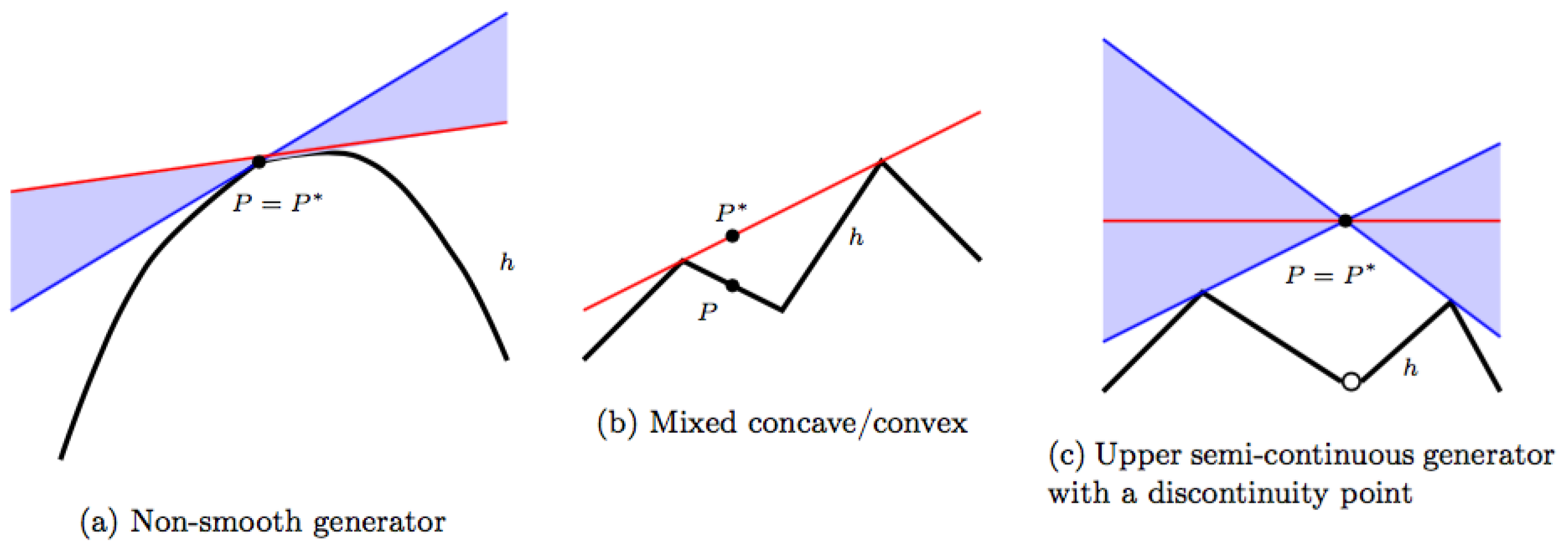
Our construction allows us to define a pretty natural information triple associated with any generalized generator. We simply define and for by
and can then assert as follows:
Theorem A1.
With the definitions (A4) and (A5), is a -proper effort-based information triple over . The triple has affine marginals .
With the thorough preparations, this is evident.
If , i.e., if h is concave, our construction has some merits over the standard Bregman construction as smoothness is not required.
Regarding the assumption that I is open, this can be dispensed with at the cost of some comments on degenerate control lines, lines which really only give control at one of the endpoints. This may be formulated by allowing infinite values for the controls or one may focus on decompositions of into two convex sets. We leave it to the reader to work this out (and to modify the proof of Lemma A1 accordingly, working separately to the left of Q and to the right of Q).
As a trivial but illuminating example when working with a closed rather than an open interval we take and as generator consider the identity map h on I. Then h itself is a control and we realize that for all u with whereas the constant control given by for all is the response to . You realize that with this generator, the associated information triple is not -proper, but it is -proper and it also satisfies the other property demanded of what we called standard properness, viz., that the optimal control is robust.
Among issues and further possibilities depending on the construction in this appendix we point to a few:
Clearly, one may “change sign” and discuss utility-based systems. This involves notion of support lines and minimal-risk supports.
Then, just as with standard Bregman constructions, one should deal with the more involved geometric complications when functions over (convex) areas in finite dimensional Euclidean spaces are involved.
One may replace h, first with its graph (in fact done), but further with any subset of . More generally, you may consider subsets G of a separable Hilbert space provided with a hyperplane and a choice of direction orthogonal to . The hyperplane is a replacement for the abscisse-axes of our discussion and the direction a replacement for the ordinate-axes. For such systems, height over the hyperplane will be a replacement for function values.
It does appear quite natural to allow continuous and concave, but not necessarily smooth generators. For instance, you may consider the generator on . In that case, it is easy to find examples to demonstrate that this generator is not -negative definite. Then, according to Proposition 11, the Jensen-Shannon divergence jsd associated with this generator is not the square of a metric. Elaborating a bit on this in a pretty natural manner, one finds that:
Proposition A1.
No Jensen-Shannon divergence constructed from a generator with bends can be the square of a metric.
Though not that surprising, this result supports the view that the attractive cases when Jensen-Shannon divergence is in fact a squared metric—perhaps even related via embedding to a squared Hilbert metric—requires a strong degree of smoothness for an underlying generator.
Appendix B. Protection against Misinformation
We present a possible variation of the interpretations emphasized in Section 2 of our study. This involves a theme which has been important for the development of the notion of proper score functions. For this appendix, is assumed.
In a sense, what we shall discuss here is what happens if Nature can communicate. Then we speak instead about Expert. Moreover, Observer becomes Customer. Expert holds the truth, x, or rather, x represents Experts best evaluation of what the truth is. Customer wants to know what Expert thinks about a certain situation and asks Expert for advice—against payment, to be agreed upon. For despicable reasons, Expert may be tempted to advice against better knowing, i.e., to give as advice y, instead of the honest advice x. Misinformation could either be due to the difficulty Expert may have in reaching a true expert opinion or it could be out of self-interest, with Expert taking advantage of false information given to Customer. Or Expert may try to mislead Customer in order to hide a business secret.
We assume that truth will be revealed to both Expert and Customer soon after Expert has given advice to Customer and further, that a proper effort function is known to both Expert and Customer. We shall device a payment scheme which will protect Customer against misinformation. The idea is simple. At the time of signing a contract—before advice is given—Customer pays a flat sum to Expert and further, Expert and Customer agree on an insurance scheme stipulating a penalty to be payed by Expert to Customer proportional to where represents what really happened and y is the advice given. If Expert is confident that he knows what will happen, he will assume that will hold and it will be in his own interest to give to Customer the honest advice .
In the literature this scheme is mainly considered based on a proper score function, the same as a proper utility function. This gives an obvious variation of the payment scheme with the score function determining payment from Customer to Expert. The most often treated situation is probably that of weather forecasting with Brier [42] the first and Weijs and Giesen [105] a recent contribution. However, also situations from economy and statistics have been studied frequently. Apart from sources just cited we refer to the sources pointed to in Section 2.6 and to McCarthy [106] as well as to Chambers [107]. As a final reference we point to Hilden [108] where applications to diagnostics is discussed.
Works cited and their references will reveal a rich literature. With access to our abstract modeling, further meaningful applications, not necessarily tied to probabilistic modeling may emerge.
Appendix C. Cause and Effect
We present one further possible variation of the interpretations emphasized in Section 2 of our study. We assume that and put . Elements of X are now interpreted as causes and response, considered as a map defined on X, as the transformation of a cause into its associated consequence. This change moves the focus from Observer’s thoughts as discussed in Section 2.3 to a reflection of causality in Nature. The set-up is in this way conceived as a model of cause and effect.
Previously we considered possible choices of Observer in - or -type games. Now it is more pertinent to focus on consequences—elements of W—as possible observations by Observer of the effect of the actual cause. For and , is now be interpreted as the cost to Observer if he has observed (or believes to have observed) the effect w when the actual cause is x.
Consider the game , say with preparation . With the new interpretation in mind it appears particularly pertinent to consider Observer’s risk associated with the various possible observations.
Concrete situations where the change of interpretation makes sense, involve information theoretical problems of capacity.
Appendix D. Negative Definite Kernels and Squared Metrics
The result needed for the proof of Proposition 11 is a simple fact leading up to a group of rather deep results, see e.g., Chapter 6 of Deza and Laurent [103] (note that there, negative definiteness is referred to as being of negative type). For the convenience of the reader we present a simple direct proof of the needed more primitive result:
Proposition A2.
Let X be an abstract set and a “kernel” which is sound (), proper ( if ) and symmetric (). Then D is a squared metric if and only if D is negative definite over three-element sets, i.e., if and only if, for any scalers with and any set of elements in X, the sum is non-positive.
Proof.
“only if”: Assume that with d a metric on X. With and and , one finds that . The second order polynomium in the parenthesis has the discriminant which is non-positive as (consider separately the cases and ). Thus S is non-positive.
“if”: With given, put and . As the sum S is non-positive with scalers of the form we find from previous calculations that from which the desired triangle inequality follows. ☐
References
- Shannon, C.E. A mathematical theory of communication. Bell Syst. Tech. J. 1948, 27, 379–423, 623–656. [Google Scholar] [CrossRef]
- Tsallis, C. Possible generalization of Boltzmann-Gibbs statistics. J. Stat. Phys. 1988, 52, 479–487. [Google Scholar] [CrossRef]
- Tsallis, C. Introduction to Nonextensive Statistical Mechanics; Springer: Berlin/Heidelberg, Germany, 2009. [Google Scholar]
- Gross, D. Comment on: “Nonextensivity: From low-dimensional maps to Hamiltonian systems” by Tsallis et al. arXiv, 2002; arXiv:cond-mat/0210448. [Google Scholar]
- Ingarden, R.S.; Urbanik, K. Information without probability. Colloq. Math. 1962, 9, 131–150. [Google Scholar]
- Kolmogorov, A.N. Logical basis for information theory and probability theory. IEEE Trans. Inf. Theory 1968, 14, 662–664. [Google Scholar] [CrossRef]
- Kolmogorov, A.N. Combinatorial foundations of information theory and the calculus of probabilities. Russ. Math. Surv. 1983, 38, 29–40. [Google Scholar] [CrossRef]
- de Fériet, K. La theorie génerélisée de l’information. In Théories de L’information (Colloq. Iiformation et Questionnaires, Marseille-Luminy, 1973); Springer: Berlin, Germany, 1974; pp. 1–35. (In French) [Google Scholar]
- Jaynes, E.T. Probability Theory—The Logic of Science; Cambridge University Press: Cambridge, UK, 2003. [Google Scholar]
- Amari, S.; Nagaoka, H. Methods of Information Geometry; Translations of Mathematical Monographs. 191; American Mathematical Society, Oxford University Press: New York, NY, USA, 1985. [Google Scholar]
- Anthonis, B. Extension of Information Geometry for Modelling Non-Statistical Systems. Ph.D. Thesis, Universiteit Antwerpen, Antwerp, Belgium, 2014. [Google Scholar]
- Rathmanner, S.; Hutter, M. A Philosophical Treatise of Universal Induction. Entropy 2011, 13, 1076–1136. [Google Scholar] [CrossRef]
- Barron, A.; Rissanen, J.; Yu, B. The Minimum Description Length Principle in Coding and Modeling. IEEE Trans. Inf. Theory 1998, 44, 2743–2760. [Google Scholar] [CrossRef]
- Grünwald, P.D. The Minimum Description Length Principle; MIT Press: Cambridge, MA, USA, 2007. [Google Scholar]
- Jumarie, G. Maximum Entropy, Information without Probability and Complex Fractals—Classical and Quantum Approach; Kluwer: Dordrecht, The Netherlands, 2000. [Google Scholar]
- Shafer, G.; Vovk, V. Probability and Finance. It’s Only a Game! Wiley: Chichester, UK, 2001. [Google Scholar]
- Gernert, D. Pragmatic Information: Historical Exposition and General Overview. Mind Matter 2006, 4, 141–167. [Google Scholar]
- Bundesen, C.; Habekost, T. Principles of Visual Attention; Oxford University Press: Oxford, UK, 2008. [Google Scholar]
- Benedetti, F. Placebo Effects. Understanding the Mechanisms in Health and Disease; Oxford University Press: Oxford, UK, 2009. [Google Scholar]
- Brier, S. Cybersemiotics: An Evolutionary World View Going Beyond Entropy and Information into the Question of Meaning. Entropy 2010, 12, 1902–1920. [Google Scholar] [CrossRef]
- Van Benthem, J.; Adriaans, P. (Eds.) Handbook on the Philosophy of Information; Handbook of the Philosophy of Science; Elsivier: Amsterdam, The Netherlands, 2007; Volume 8. [Google Scholar]
- Adriaans, P. Information. Stanford Encyclopedia of Philosophy, 2012; p. 43. Available online: http://plato.stanford.edu/archives/fall2013/entries/information/ (accessed on 26 March 2017).
- Brier, S. Cybersemiotics: Why Information Is Not Enough; Toronto University Press: Toronto, ON, Canada, 2008. [Google Scholar]
- Topsøe, F. Game Theoretical Equilibrium, Maximum Entropy and Minimum Information Discrimination. In Maximum Entropy and Bayesian Methods; Mohammad-Djafari, A., Demoments, G., Eds.; Kluwer Academic Publishers: Dordrecht, The Netherlands; Boston, MA, USA; London, UK, 1993; pp. 15–23. [Google Scholar]
- Pfaffelhuber, E. Minimax Information Gain and Minimum Discrimination Principle. In Topics in Information Theory, Proceedings of the Colloquia Mathematica Societatis János Bolyai, Oberwolfach, Germany, 13–23 April 1977; Csiszár, I., Elias, P., Eds.; János Bolyai Mathematical Society and North-Holland: Amsterdam, The Netherlands; Oxford, UK; New York, NY, USA, 1977; Volume 16, pp. 493–519. [Google Scholar]
- Topsøe, F. Information Theoretical Optimization Techniques. Kybernetika 1979, 15, 8–27. [Google Scholar]
- Harremoës, P.; Topsøe, F. Maximum Entropy Fundamentals. Entropy 2001, 3, 191–226. [Google Scholar] [CrossRef]
- Grünwald, P.D.; Dawid, A.P. Game Theory, Maximum Entropy, Minimum Discrepancy, and Robust Bayesian Decision Theory. Ann. Math. Stat. 2004, 32, 1367–1433. [Google Scholar]
- Friedman, C.; Jinggang, H.; Sandow, S. A Utility-Based Approach to Some Information Measures. Entropy 2007, 9, 1–26. [Google Scholar] [CrossRef]
- Dayi, H. Game Analyzing based on Strategic Entropy. Chin. J. Manag. Sci. 2009, 17, 133–138. (In Chinese) [Google Scholar]
- Harremoës, P.; Topsøe, F. The Quantitative Theory of Information. In Handbook on the Philosophy of Information; van Benthem, J., Adriaans, P., Eds.; Handbook of the Philosophy of Science; Elsivier: Amsterdam, The Netherlands, 2008; Volume 8, pp. 171–216. [Google Scholar]
- Aubin, J.P. Optima and Equilibria. An Introduction to Nonlinear Analysis; Springer: Berlin, Germany, 1993. [Google Scholar]
- Cesa-Bianchi, N.; Lugosi, G. Prediction, Learning and Games; Cambridge University Press: Cambridge, UK, 2006. [Google Scholar]
- Topsøe, F. Interaction between Truth and Belief as the key to entropy and other quantities of statistical physics. arXiv, 2008; arXiv:0807.4337v1. [Google Scholar]
- Topsøe, F. Truth, Belief and Experience—A route to Information. J. Contemp. Math. Anal. Armen. Acad. Sci. 2009, 44, 105–110. [Google Scholar] [CrossRef]
- Topsøe, F. On truth, belief and knowledge. In Proceedings of the 2009 IEEE International Symposium on Information Theory, Seoul, Korea, 28 June–3 July 2009; pp. 139–143. [Google Scholar]
- Topsøe, F. Towards operational interpretations of generalized entropies. J. Phys. Conf. Ser. 2010, 201, 15. [Google Scholar] [CrossRef]
- Topsøe, F. Elements of the Cognitive Universe. Available online: http://www.math.ku.dk/~topsoe/isit2011.pdf (accessed on 31 March 2017).
- Wikipedia. Bayesian Probability—Wikipedia, The Free Encyklopedia. 2009. Available online: https://en.wikipedia.org/wiki/Bayesian_Probability (accessed on 31 January 2011).
- Good, I.J. Rationel Decisions. J. R. Stat. Soc. Ser. B 1952, 14, 107–114. [Google Scholar]
- Csiszár, I. Axiomatic Characterizations of Information Measures. Entropy 2008, 10, 261–273. [Google Scholar] [CrossRef]
- Brier, G.W. Verification of forecasts expressed in terms of probability. Mon. Weather Rev. 1950, 78, 1–3. [Google Scholar] [CrossRef]
- Savage, L.J. Elicitation of Personal Probabilities and Expectations. J. Am. Stat. Assoc. 1971, 66, 783–801. [Google Scholar] [CrossRef]
- Fischer, P. On the Inequality ∑ pif(pi) ≥ ∑ pif(qi). Metrika 1972, 18, 199–208. [Google Scholar] [CrossRef]
- Gneiting, T.; Raftery, A.E. Strictly Proper Scoring Rrules, Prediction, and Estimation. J. Am. Stat. Assoc. 2007, 102, 359–378. [Google Scholar] [CrossRef]
- Dawid, A.P.; Lauritzen, S.L. The geometry of decision theory. In Proceedings of the Second International Symposium on Information Geometry and its Applications, Tokyo, Japan, 12–16 December 2006; pp. 22–28. [Google Scholar]
- Dawid, A.P.; Musio, M. Theory and Applications of Proper Scoring Rules. Metron 2014, 72, 169–183. [Google Scholar] [CrossRef]
- Philip, A.; Dawid, M.M.; Ventura, L. Minimum Scoring Rule Inference. Scand. J. Stat. 2016, 43, 123–138. [Google Scholar]
- Caticha, A. Information and Entropy. In Bayesian Inference and Maximum Entropy Methods in Science and Engineering: 27th International Workshop on Bayesian Inference and Maximum Entropy Methods; American Institute of Physics Inc.: Woodbury, NY, USA, 2007; Volume 954, pp. 11–22. [Google Scholar]
- Kerridge, D.F. Inaccuracy and inference. J. R. Stat. Soc. B 1961, 23, 184–194. [Google Scholar]
- Kullback, S. Information Theory and Statistics; Wiley: New York, NY, USA, 1959. [Google Scholar]
- Rubin, E. Om Forstaaelighedsreserven og om Overbestemthed. In Til Minde om Edgar Rubin; Nordisk Psykologisk Monografiserie NR. 8: Copenhagen, Denmark, 1956; pp. 28–37. (In Danish) [Google Scholar]
- Rasmussen, E.T. Bemærkninger om E. Rubin’s “reserve-begreb”. In Til Minde om Edgar Rubin; Nordisk Psykologisk Monografiserie NR. 8: Copenhagen, Denmark, 1956; pp. 38–42. [Google Scholar]
- Boyd, S.; Vandenberghe, L. Convex Optimization; Cambridge University Press: Cambridge, UK, 2004. [Google Scholar]
- Topsøe, F. Game theoretical optimization inspired by information theory. J. Glob. Optim. 2009, 43, 553–564. [Google Scholar] [CrossRef]
- Zeidler, E. Applied Mathematical Sciences. In Applied Functional Analysis: Applications to Mathematical Physics; Springer: New York, NY, USA, 1995; Volume 108. [Google Scholar]
- Zeidler, E. Applied Mathematical Sciences. In Applied Functional Analysis: Main Principles and Their Applications; Springer: Berlin, Germany, 1995; Volume 109. [Google Scholar]
- Von Neumann, J. Zur Theorie der Gesellschaftsspiele. Math. Ann. 1928, 100, 295–320. [Google Scholar] [CrossRef]
- Von Neumann, J. Über ein ökonomische Gleichungssystem und eine Veralgemeinerung des Brouwerschen Fixpunktsatzes. Ergeb. Math. Kolloqu. 1937, 8, 73–83. (In German) [Google Scholar]
- Kjeldsen, T.H. John von Neumann’s Conception of the Minimax Theorem: A Journey Through Different Mathematical Contexts. Arch. Hist. Exact Sci. 2001, 56, 39–68. [Google Scholar] [CrossRef]
- Kuic, D. Maximum information entropy principle and the interpretation of probabilities in statistical mechanics—A short review. Eur. Phys. J. B 2016, 89, 1–7. [Google Scholar] [CrossRef]
- Topsøe, F. Exponential Families and MaxEnt Calculations for Entropy Measures of Statistical Physics. In Complexity, Metastability, and Non-Extensivity, CTNEXT07; AIP Conference Proceedings; American Institute of Physics: New York, NY, USA, 2007; Volume 965, pp. 104–113. [Google Scholar]
- Csiszár, I. I-Divergence Geometry of Probability Distributions and Minimization Problems. Ann. Probab. 1975, 3, 146–158. [Google Scholar] [CrossRef]
- Čencov, N.N. Statistical Decision Rules and Optimal Inference; In Russian, Translation in “Translations of Mathematical Monographs”; American Mathematical Society: Providence, RI, USA, 1982; Nauka: Moscow, Russia, 1972. [Google Scholar]
- Csiszár, I. Generalized projections for non-negative functions. Acta Math. Hung. 1995, 68, 161–185. [Google Scholar] [CrossRef]
- Csiszár, I.; Matús, F. Information projections revisited. IEEE Trans. Inf. Theory 2003, 49, 1474–1490. [Google Scholar] [CrossRef]
- Csiszár, I.; Matús, F. Generalized minimizers of convex integral functionals, Bregman distance, Pythagorean identities. Kybernetika 2012, 48, 637–689. [Google Scholar]
- Glonti, O.; Harremoës, P.; Khechinashili, Z.; Topsøe, F. Nash Equilibrium in a Game of Calibration. Theory Probab. Appl. 2007, 51, 415–426. [Google Scholar] [CrossRef]
- Topsøe, F. Basic Concepts, Identities and Inequalities—The Toolkit of Information Theory. Entropy 2001, 3, 162–190. [Google Scholar] [CrossRef]
- Endres, D.M.; Schindelin, J.E. A new metric for probability distributions. IEEE Trans. Inf. Theory 2003, 49, 1858–1860. [Google Scholar] [CrossRef]
- Fuglede, B.; Topsøe, F. Jensen-Shannon Divergence and Hilbert space Embedding. In Proceedings of the 2004 International Symposium on Information Theory, Honolulu, HW, USA, 29 June–4 July 2014; p. 31. [Google Scholar]
- Briët, J.; Harremoës, P. Properties of Classical and Quantum Jensen-Shannon Divergence. Phys. Rev. A 2009, 79, 11. [Google Scholar] [CrossRef]
- Kisynski, J. Convergence du typè L. Colloq. Math. 1960, 7, 205–211. [Google Scholar]
- Dudley, R. On Sequential Convergence. Trans. Am. Math. Soc. 1964, 112, 483–507. [Google Scholar] [CrossRef]
- Steen, L.; Seebach, J. Counterexamples in Topology; Springer: Berlin, Germany, 1941. [Google Scholar]
- Harremoës, P.; Topsøe, F. Zipf’s law, hyperbolic distributions and entropy loss. In Proceedings of the IEEE International Symposium on Information Theory, Lausanne, Switzerland, 30 June–5 July 2002; p. 207. [Google Scholar]
- Bregman, L.M. The relaxation method of finding the common point of convex sets and its application to the solution of problems in convex programming. USSR Comput. Math. Math. Phys. 1967, 7, 200–217. [Google Scholar] [CrossRef]
- Tsallis, C. What are the numbers that experiments provide? Quim. Nova 1994, 17, 468. [Google Scholar]
- Csiszár, I. Eine informationstheoretische Ungleichung und ihre anwendung auf denBeweis der ergodizität von Markoffschen Ketten. Publ. Math. Inst. Hung. Acad. 1963, 8, 95–108. [Google Scholar]
- Morimoto, T. Markov processes and the H-theorem. J. Phys. Soc. Jpn. 1963, 12, 328–331. [Google Scholar] [CrossRef]
- Ali, S.M.; Silvey, S.D. A General Class of Coefficients of Divergence of One Distribution from Another. J. R. Stat. Soc. Ser. B 1966, 28, 131–142. [Google Scholar]
- Havrda, J.; Charvát, F. Quantification method of classification processes. Concept of structural a-entropy. Kybernetika 1967, 3, 30–35. [Google Scholar]
- Daróczy, Z. Generalized Information Functions. Inf. Control 1970, 16, 36–51. [Google Scholar] [CrossRef]
- Lindhard, J.; Nielsen, V. Studies in Statistical Dynamics. Det Kongelige Danske Videnskabernes Selskab Matematisk-Fysiske Meddelelser 1971, 38, 1–42. [Google Scholar]
- Lindhard, J. On the Theory of Measurement and its Consequences in Statistical Dynamics. Det Kongelige Danske Videnskabernes Selskab Matematisk-Fysiske Meddelelser 1974, 39, 1–39. [Google Scholar]
- Aczél, J.; Daróczy, Z. On Measures of Information and Their Characterizations; Academic Press: New York, NY, USA, 1975. [Google Scholar]
- Ebanks, B.; Sahoo, P.; Sander, W. Characterizations of Information Measures; World Scientific: Singapore, 1998. [Google Scholar]
- Jaynes, E.T. Where do we Stand on Maximum Entropy? In The Maximum Entrropy Formalism; Levine, R., Tribus, M., Eds.; MIT Press: Cambridge, MA, USA, 1979; pp. 1–104. [Google Scholar]
- Naudts, J. Generalised exponential families and associated entropy functions. Entropy 2008, 10, 131–149. [Google Scholar] [CrossRef]
- Gallager, R. Information Theory and Reliable Communication; Wiley: New York, NY, USA, 1968. [Google Scholar]
- Topsøe, F. Informationstheorie, eine Einführung; Teubner: Stuttgart, Germany, 1974. [Google Scholar]
- Sylvester, J.J. A Question in the Geometry of Situation. Q. J. Pure Appl. Math. 1857, 1, 79. [Google Scholar]
- Drezner, Z.; Hamacher, H. (Eds.) Facility Location. Applications and Theory; Springer: Berlin, Germany, 2002. [Google Scholar]
- Topsøe, F. A New Proof of a Result Concerning Computation of the Capacity for a Discrete Channel. Zeitschrift für Wahrscheinlichkeitstheorie und Verwandte Gebiete 1972, 22, 166–168. [Google Scholar] [CrossRef]
- Van der Lubbe, J.C.A. Transactions of the Prague Conferences on Information Theory. In On Certain Coding Theorems for the Information of Order α and of type β; Springer: Dordrecht, The Netherlands, 1979. [Google Scholar]
- Ahlswede, R. Identification Entropy. In General Theory of Information Transfer and Combinatorics; Lecture Notes in Computer Science; Springer: Berlin, Germany, 2006; Volume 4123, pp. 595–613. [Google Scholar]
- Suyari, H. Tsallis entropy as a lower bound of average description length for the q-generalized code tree. In Proceedings of the IEEE International Symposium on Information Theory (ISIT 2007), Nice, France, 24–29 June 2007; pp. 901–905. [Google Scholar]
- Topsøe, F. Factorization and escorting in the game-theoretical approach to non-extensive entropy measures. Physica A 2006, 365, 91–95. [Google Scholar] [CrossRef]
- Tsallis, C. Conceptual Inadequacy of the Shore and Johnson Axioms for Wide Classes of Complex Systems. Entropy 2015, 17, 2853–2861. [Google Scholar] [CrossRef]
- Kapur, J.N. Maximum Entropy Models in Science and Engineering; First Edition 1989; Wiley: New York, NY, USA, 1993. [Google Scholar]
- Topsøe, F. Maximum Entropy versus Minimum Risk and Applications to some classical discrete Distributions. IEEE Trans. Inf. Theory 2002, 48, 2368–2376. [Google Scholar] [CrossRef]
- Pavon, M.; Ferrante, A. On the Geometry of Maximum Entropy Problems. SIAM Rev. 2013, 55, 415–439. [Google Scholar] [CrossRef]
- Deza, M.M.; Laurent, M. Geometry of Cuts and Metrics; Springer: Berlin, Germany, 1997. [Google Scholar]
- Van Campenhout, J.M.; Cover, T.M. Maximum Entropy and Conditional Probability. IEEE Trans. Inf. Theory 1981, IT-27, 483–489. [Google Scholar] [CrossRef]
- Weijs, S.V.; van de Giesen, N. Accounting for Observational Uncertainty in Forecast Verification: An Information-Theoretical View on Forecasts, Observations, and Truth. Mon. Weather Rev. 2011, 139, 2156–2162. [Google Scholar] [CrossRef]
- McCarthy, J. Measures of the Value of Information. Proc. Natl. Acad. Sci. USA 1956, 42, 654–655. [Google Scholar] [CrossRef] [PubMed]
- Chambers, C.P. Proper scoring rules for general decision models. Games Econ. Behav. 2008, 63, 32–40. [Google Scholar] [CrossRef]
- Hilden, J. Scoring Rules for Evaluation of Prognosticians and Prognostic Rules, First Version 1999; 2008, unpublished. Available online: http://publicifsv.sund.ku.dk/~jh/ (accessed on 26 March 2017).
Figure 1.
Matrix games where one of the players does not have an optimal strategy.
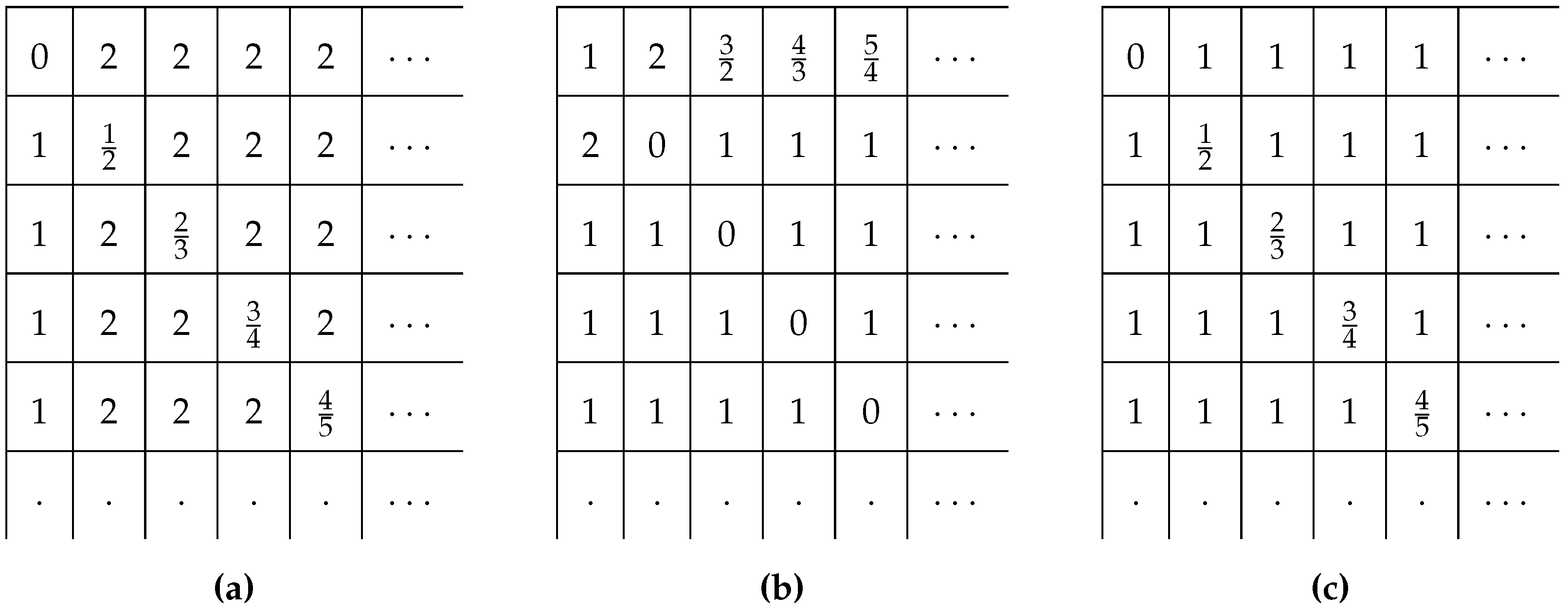
Figure 2.
Bregman generator and primitive effort-based information triple.

Figure 3.
Jensen-Shannon divergence for the Bregman construction.
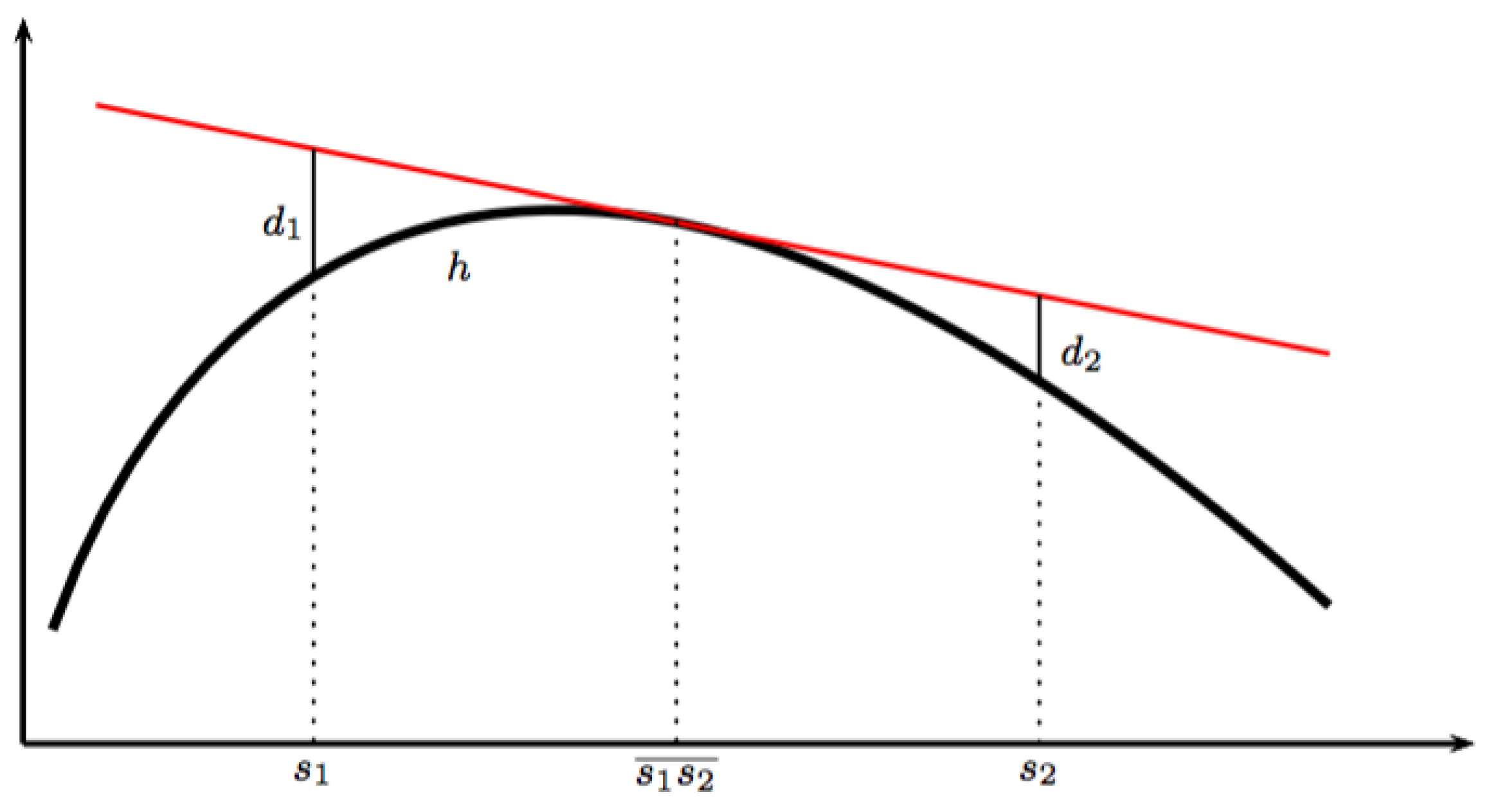
Figure 4.
Optimal strategies, typical equilibrium via core.
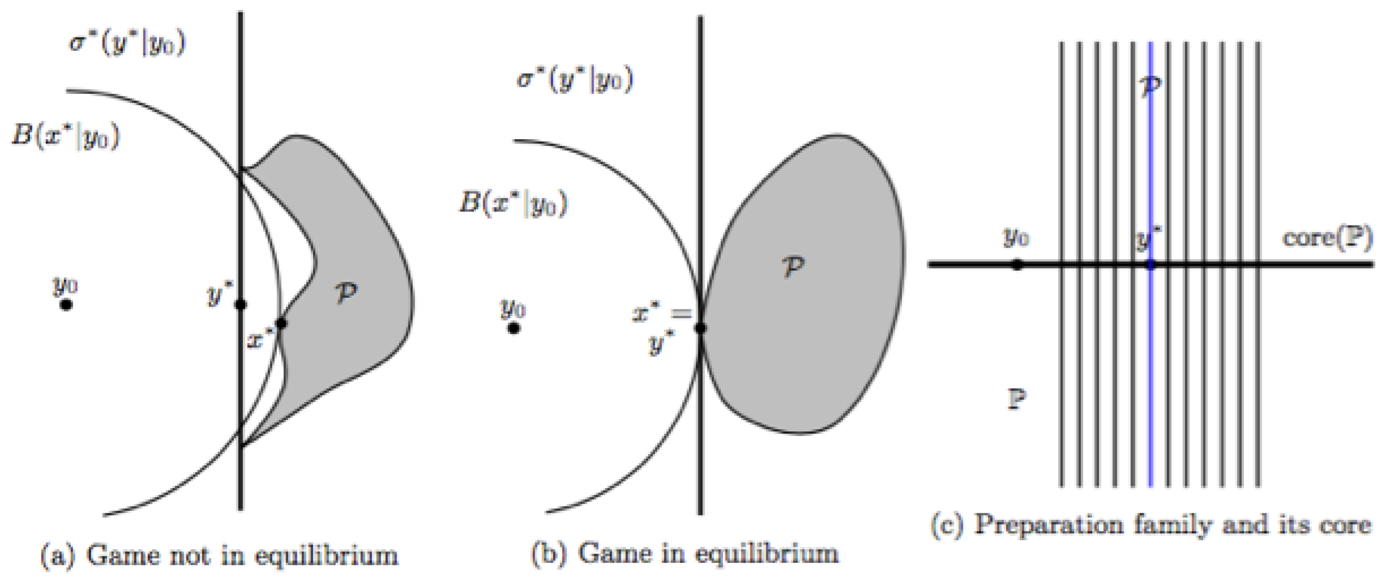
© 2017 by the author. Licensee MDPI, Basel, Switzerland. This article is an open access article distributed under the terms and conditions of the Creative Commons Attribution (CC BY) license (http://creativecommons.org/licenses/by/4.0/).
Share and Cite
MDPI and ACS Style
Topsøe, F. Paradigms of Cognition. Entropy 2017, 19, 143. https://doi.org/10.3390/e19040143
AMA Style
Topsøe F. Paradigms of Cognition. Entropy. 2017; 19(4):143. https://doi.org/10.3390/e19040143
Chicago/Turabian StyleTopsøe, Flemming. 2017. "Paradigms of Cognition" Entropy 19, no. 4: 143. https://doi.org/10.3390/e19040143
APA StyleTopsøe, F. (2017). Paradigms of Cognition. Entropy, 19(4), 143. https://doi.org/10.3390/e19040143
Note that from the first issue of 2016, this journal uses article numbers instead of page numbers. See further details here.