
Carnot-Like Heat Engines Versus Low-Dissipation Models
by

Julian Gonzalez-Ayala
1,*, 
José Miguel M. Roco
1,2, 
Alejandro Medina
1 and
Antonio Calvo Hernández
1,2,* 1
Departamento de Física Aplicada, Universidad de Salamanca, 37008 Salamanca, Spain
2
Instituto Universitario de Física Fundamental y Matemáticas (IUFFyM), Universidad de Salamanca, 37008 Salamanca, Spain
*
Authors to whom correspondence should be addressed.
Entropy 2017, 19(4), 182; https://doi.org/10.3390/e19040182
Submission received: 20 March 2017
/
Revised: 18 April 2017
/
Accepted: 20 April 2017
/
Published: 23 April 2017
(This article belongs to the Special Issue Carnot Cycle and Heat Engine Fundamentals and Applications)
Abstract
:In this paper, a comparison between two well-known finite time heat engine models is presented: the Carnot-like heat engine based on specific heat transfer laws between the cyclic system and the external heat baths and the Low-Dissipation model where irreversibilities are taken into account by explicit entropy generation laws. We analyze the mathematical relation between the natural variables of both models and from this the resulting thermodynamic implications. Among them, particular emphasis has been placed on the physical consistency between the heat leak and time evolution on the one side, and between parabolic and loop-like behaviors of the parametric power-efficiency plots. A detailed analysis for different heat transfer laws in the Carnot-like model in terms of the maximum power efficiencies given by the Low-Dissipation model is also presented.
1. Introduction
A cornerstone in thermodynamics is the analysis of the performance of heat devices. Since the Carnot’s result about the maximum possible efficiency that any heat converter operating between two heat reservoirs might reach, the work in this field is mainly focused on how to fit real-life devices as close as possible to the main requirement behind the Carnot efficiency value, i.e., the existence of infinite-time, quasi-static processes. However, real-life devices work under finite-time and finite-size constraints, thus giving finite power output. Over the last several decades, one of the most popular models in the physics literature to analyze finite-time and finite-size heat devices has been the so-called Carnot-like model. Inspired by the work reported by Curzon–Ahlborn (CA) [1], this model provides a first valuable approach to the behavior of real heat engines.
In this model, it is assumed an internally reversible Carnot cycle coupled irreversibly with two external thermal reservoirs (endoreversible hypothesis) through some heat transfer laws and some phenomenological conductances related with the nature of the heat fluxes and the properties of the materials and devices involved in the transport phenomena. Without any doubt, the main result was the so-called CA-efficiency (where is the ratio of the external cold and hot heat reservoirs). It accounts for the efficiency at maximum–power (MP) conditions when the heat transfer laws are considered linear with the temperature difference between the external heat baths and the internal temperatures of the isothermal processes at which the heat absorption and rejection occurs. Later extensions of this model included the existence of a heat leak between the two external baths and the addition of irreversibilities inside of the internal cycle. With only three main ingredients (heat leak, external coupling, and internal irreversibilities) the Carnot-like model has been used as a paradigmatic model to confront many research results coming from macroscopic, mesoscopic and microscopic fields [1,2,3,4,5,6,7,8,9,10,11,12,13,14,15,16,17,18,19,20,21,22,23,24,25,26,27,28]. Particularly relevant have been those results concerned with the optimization not only of the power output but also of different thermodynamic and/or thermo-economic figures of merit and additionally the analysis on the universality of the efficiency at MP (or on other figures of merit as ecological type [29,30,31,32,33,34]).
Complementary to the CA-model, the Low-Dissipation (LD) model, proposed by Esposito et al. in 2009 [35], consists of a Carnot engine with small deviations from the reversible cycle through dissipations located at the isothermal branches which occur at finite-time. The nature of the dissipations (entropy generation) are encompassed in some generic dissipative coefficients, so that the optimization of power output (or any other figure of merit) is made easily through the contact times of the engine with the hot and cold reservoirs [36,37,38,39]. In this way, depending on the symmetry of the dissipative coefficients, it is possible to recover several results of the CA-model. In particular, the CA-efficiency is recovered in the LD-model under the assumption of symmetric dissipation. Recently, a description of the LD model in terms of characteristic dimensionless variables was proposed in [40,41,42]. From this treatment, it is possible to separate efficiency-power behaviors typical of CA-endoreversible engines as well as irreversible engines according to the imposed time constraints. If partial contact times are constrained, then one obtains open parabolic (endoreversible) curves; otherwise, if total time is fixed, one obtains closed loop-like curves.
The objective of this paper is to analyze in which way the Carnot-like heat engines (dependent on heat transfer laws) and the LD models (dependent on a specific entropy generation law) are related and how the variables of each one are connected. This allows for an interpretation of the heat transfer laws, including the heat leak, in terms of the bounds for the efficiency at MP provided by the LD-model, which, in turn, are dependent on the relative symmetries of the dissipations constants and the partial contact times.
The article is organized as follows: in Section 2, a correspondence among the variables of the two models for heat engines (HE) is made. In Section 3, we study the region of physically acceptable values for the Carnot-like HE variables depending on the heat leak. In Section 4, the study of the MP regime is made, showing that a variety of results between both descriptions can be recovered only in a certain range of heat transfer laws; in particular, we analyze the efficiency vs. power curves behaviors. Finally, some concluding remarks are presented in Section 5.
2. Correspondence between the HE’s Variables of Both Models
A key point to establish the linkage between both models is the entropy production. By equaling the entropy change stemming from both frameworks it is possible to give the relations among the variables that describe each model (see Figure 1).
In the LD case (see Figure 1a), the base-line Carnot cycle works between the temperatures and , the entropy change along the hot (cold) isothermal path is () and the times to complete each isotherm processes are and , respectively. The adiabatic processes, as usual, are considered as instantaneous, though the influence of finite adiabatic times has been reported in the LD-model in [43]. The deviation from the reversible scenario in the LD approximation is considered by an additional contribution to the entropy change at the hot and cold reservoirs given by
where and are the so-called dissipative coefficients. The signs take into account the direction of the heat fluxes from (toward) the hot (cold) reservoir in such a way that and are positive quantities. Then, the total entropy generation is given by
At this point, it is helpful to use the dimensionless variables defined in [40]: , and , where and . In this way, it is possible to define a characteristic total entropy production per unit time for the LD-model as
In the irreversible Carnot-like HE, the entropy generation of the internal reversible cycle is zero and the total entropy production is that generated at the external heat reservoirs (see Figure 1b). By considering the same sign convention as in the LD model and , where is the entropy change in the hot isothermal branch of the reversible Carnot cycle, and a heat leak between the reservoirs and , then
where and . By introducing a characteristic heat leak and a comparison with Equations (1) and (2) gives the expressions associated with the dissipations
By assuming that the ratio is the same in both descriptions, then we introduce into the Carnot-like model, and and are
which are the relations between the characteristic variables of the LD model and the variables of the Carnot-like HE. This is summarized in the following expression:
3. Physical Space of the HE Variables
We stress that all the above results between variables hold for arbitrary heat transfer laws in the Carnot-like model. As a consequence, above equations provide the generic linkage between both descriptions, and, from them, useful thermodynamic information can be extracted.
In Figure 2a, the internal temperatures for the irreversible Carnot-like HE, contained in and , are depicted with fixed values , and . Notice that, in order to obtain thermal equilibrium between the auxiliary reservoirs and the external baths (i.e., to achieve the reversible limit), it is necessary that . As soon as a heat leak appears, , meanwhile is always a possible configuration. As the heat leak increases in the HE, the internal temperatures get closer to each other until the limiting situation where (see contact edge in Figure 2a).
As a heat leak appears, the reversible limit is no longer achievable. This is better reflected in Figure 2b, where we plot the total operation time depending on and (see Equation (11)). Only when and can large operation times be allowed. We can see in this figure that the existence of a heat leak imposes a maximum operational characteristic time to the HE. The total time is noticeably shorter as the heat leak increases, in agreement with the fact that, for the working regimes are dominated by dissipations. It could be said that the heat leak behaves as a causality effect in the arrow of time of the heat engine.
Notice that, in Figure 2, there is a region of prohibited combinations of and . This has to do with the physical reality of the engine (negative power output and efficiency). In [41], the region of physical interest in the LD model under maximum power conditions was analyzed. In the Carnot-like engine, some similar considerations can be addressed as follows: in a valid endoreversible HE, the internal temperatures may vary in the range and in order to have , being the condition for implying null work output and efficiency. From Equation (9), it is possible to obtain two conditions on (initially assumed to be ) according to the values and . For we obtain that
whose only physical solution is . Then, as long as there is a heat leak in the device, the internal hot reservoir cannot reach equilibrium with the external hot reservoir and the reversible configuration is not achievable. On the other hand (as can be seen in Figure 2a), the largest possible heat leak (i.e., the largest dissipation in the system) has as an outcome that , that is, and . In that limit, Equations (9) and (11) give
and, since in this case all the input heat is dissipated to the cold external thermal reservoir, the HE has a null power output. In Figure 3, we depict the range of possible values that can take (from 0 up to ) in terms of and . By means of Equation (13), it is established a boundary condition for physically acceptable values of the irreversible Carnot-like HE in terms of the LD variables, which is
Up to this point, we have proposed a generic correspondence between the variables of both schemes: the LD treatment, based on a specific entropy generation law, and the irreversible Carnot-like engine based on heat transfer laws. In the following, we will further analyze the connection given by Equation (11) with the focus on different heat transfer laws and the maximum power efficiencies given by the low-dissipation model.
4. Maximum-Power Regime
As is usual, the power output is given by
In [41], it was shown that, in the MP regime of an LD engine display, an open, parabolic behavior for the parametric curves when is fixed and for . On the other hand, by fixing the value of , one obtains for the behavior of vs. P loop-like curves (see Figure 4 in [41]). In the irreversible Carnot-like framework, open vs. P curves are characteristic of endoreversible CA-type engines, and, when a heat leak is introduced, one obtains loop-like curves. The apparent connection between the behavior displayed by fixing or in the low dissipation context with the presence of a heat leak, or the lack of it, is by no means obvious. A simple analysis of the MP regime in an irreversible Carnot-like engine in terms of the LD variables will shed some light on this issue and will also provide us a better understanding of how good the correspondence is between both schemes.
4.1. Low Dissipation Heat Engine
In terms of the characteristic variables, the input and output heat are
giving a power output and efficiency as follows:
The optimization of is accomplished through the partial contact time and the total time , whose values are
with an MP efficiency given by
One of the most relevant features of this model is the capability of obtaining upper and lower bounds of the MP efficiencies without any information regarding the heat fluxes nature. These limits are
corresponding to and for the lower and upper bounds, respectively. For the symmetric dissipation case, , the well known CA-efficiency is recovered.
4.2. Carnot-Like Model without Heat Leak (Endoreversible Model)
Now, let us consider a family of heat transfer laws depending on the power of the temperature to model the heat fluxes and (see Figure 1b) as follows:
where is a real number, and are the conductances in each process and and are the times at which the isothermal processes are completed. The adiabatic processes are considered as instantaneous, a common assumption in the two models. According to Equation (15), power output is a function depending on the variables , and the ratio of contact times; k, and are not optimization variables for this model. The endoreversible hypothesis gives the following constriction upon the contact times ratio
where . Since there is no heat leak, the efficiency of the internal Carnot cycle is the same as the efficiency of the engine, then , and the dependence of is substituted by . Then, in terms of , Equation (26) is
The optimization of power output in this case is achieved through and . The maximum power is obtained by solving for and for . From the first condition, we obtain , which is
This function has a unique maximum corresponding to , which is the solution to the following equation
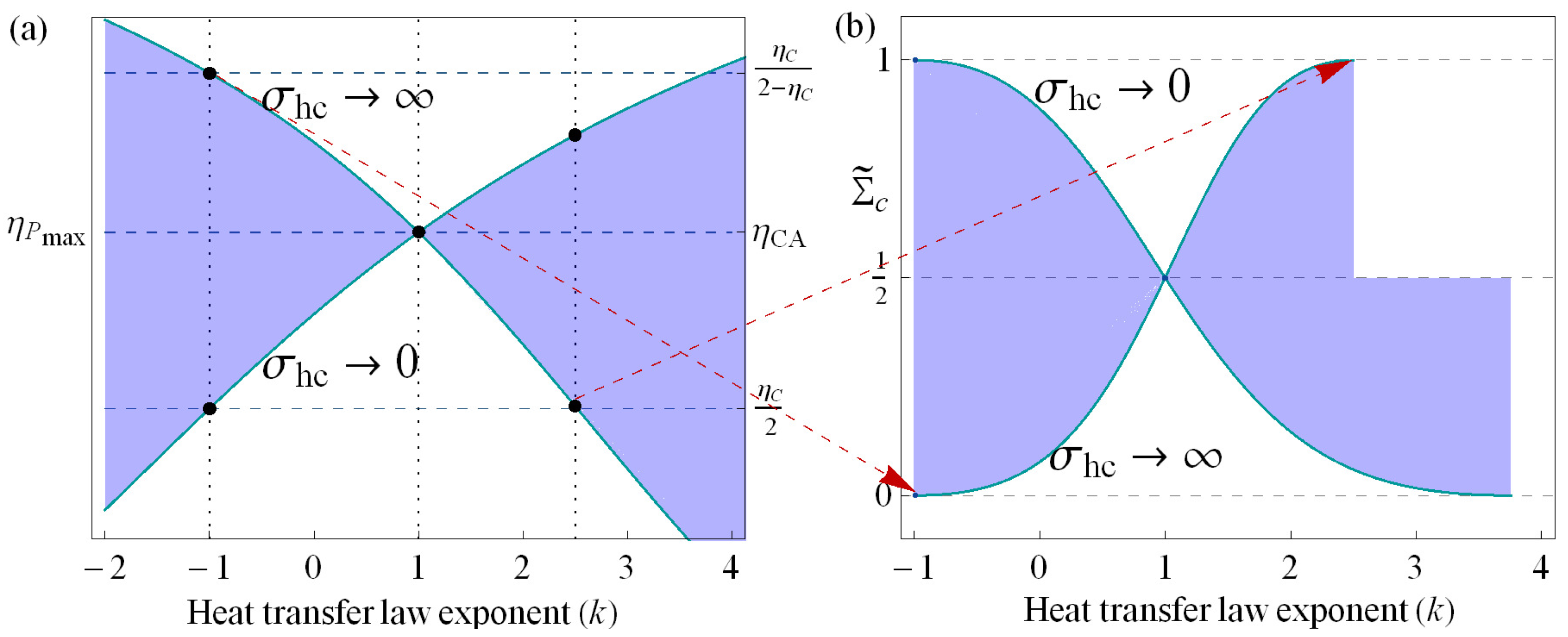
and depends on the values , and the exponent of the heat transfer law k as showed in [9]. In Figure 4a, is depicted for the limiting cases . All of the possible values of for different s are located between these two curves. It is well-known that, for the Newtonian heat transfer law (), is independent of the value. As the heat transfer law departs from the Newtonian case, the upper and lower bounds cover a wider range of efficiencies. Then, the limits appearing in Equation (23) are fulfilled for a limited region of k values in the Carnot-like model. From Figure 4a, it is possible to see that the results stemming from an endoreversible engine are accessible from an LD landmark only in the region (for other values of k, there are efficiencies outside the range given by Equation (23)). By equaling these efficiencies with the LD one (see Equation (22)) and solving for , we obtain those values that reproduce the endoreversible efficiencies. This is depicted in Figure 4b. Notice also that not all symmetries are allowed for every . For example, with a heat transfer law with exponent , all the possible values of the efficiency can be obtained if the parameter varies from 0 to 1, that is, all symmetries are allowed. Meanwhile, for , only the symmetric case is allowed, reproducing the CA efficiency. For k outside , there are efficiencies above and below the limits in Equation (23) with no values that might reproduce those efficiencies, thus limiting the heat transfer laws physically consistent with predictions of the LD model.
Inside the region where the LD model is able to reproduce the asymmetric limiting cases (), the correspondence between the two formalisms has not an exact fitting. In order to show this, we will address the symmetric dissipation case.
As can be seen from Figure 4, in the endoreversible CA-type HE, for every k, there is one that reproduces the CA efficiency. On the other hand, in the LD model, the symmetric dissipation is attached to . If we use the and values of MP of the LD model and calculate the values of and associated with them (instead of calculating them according to Equations (28) and (29)), we can see whether they allow us to recover the correct value of that in the endoreversible model gives the CA efficiency or does not. That is, for , Equations (20) and (21) reduce to
By using Equation (30), the ratio of contact times results in , and, by using the endoreversible hypothesis (Equation (26)), it is possible to obtain the value of that would produce the CA efficiency, being
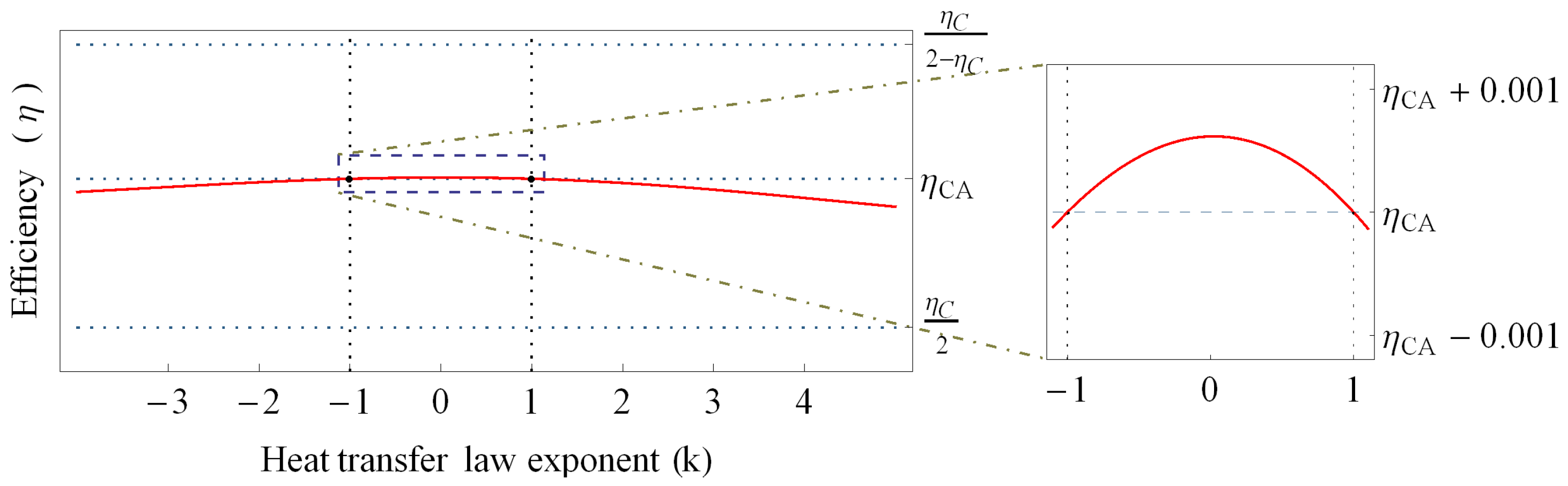
which for gives and for gives . Nevertheless, by substituting Equation (34) into Equation (29), the MP efficiency is not exactly the CA one, as can be seen in Figure 5. Showing that the correspondence between both models is a good approximation only in the range , and is exact only for and .
Another incompatibility of the two approaches comes up in the Newtonian heat exchange (): meanwhile, the Carnot-like scheme is independent of any value of , and, in terms of the LD model, is strictly attached to a symmetric dissipation . Then, the only law that has an exact correspondence for all values of and is the law .
4.3. Carnot-Like Model with Heat Leak
Now, let us consider a heat leak of the same kind of the heat fluxes and , that is,
then, the characteristic heat leak is
The power output of the engine is the same than in the endoreversible case; however, a difference with the previous subsection arises, and now the efficiency is given by the following expression:
where we have used the fact that to introduce the characteristic heats in the last expression.
From Equation (37), it can be derived that, if the heat leak increases, the efficiency diminishes. In Figure 6, we can observe how the upper and lower bounds of the efficiency appearing in Figure 4 are affected by the introduction of a constant heat leak. Now, by using Equation (37) and the fact that in the endoreversible case , we have plotted the values that leads the efficiency for (of the endoreversible case) down to the value (see point A in Figure 6), which is ; and the value that lead to an efficiency for (of the endoreversible case) to (see point B in Figure 6).
Notice in Figure 6 that, for there is a region around where is outside the shaded region of maximum power efficiencies. Then, for these values of k and , the symmetric dissipation case, always attached to the efficiency, is out of reach. Additionally, there is not a heat transfer law that fulfills both upper and lower bounds for maximum power efficiency given by the LD model as occurred for in the endoreversible case. The additional degree of freedom caused by the appearance of the heat leak makes more complex the analysis of the validity of the correspondence between both models, which, in general, should be handled numerically.
5. Conclusions
We analyzed Carnot-like heat engines (dependent on heat transfer laws) and the LD models (dependent on a specific entropy generation law) and studied how the variables of each one are connected. We were able to provide an interpretation of the heat transfer laws, including the heat leak, in terms of the bounds for the efficiency at MP provided by the LD-model, which, in turn, are dependent on the relative symmetries of the dissipations constants and the partial contact times.
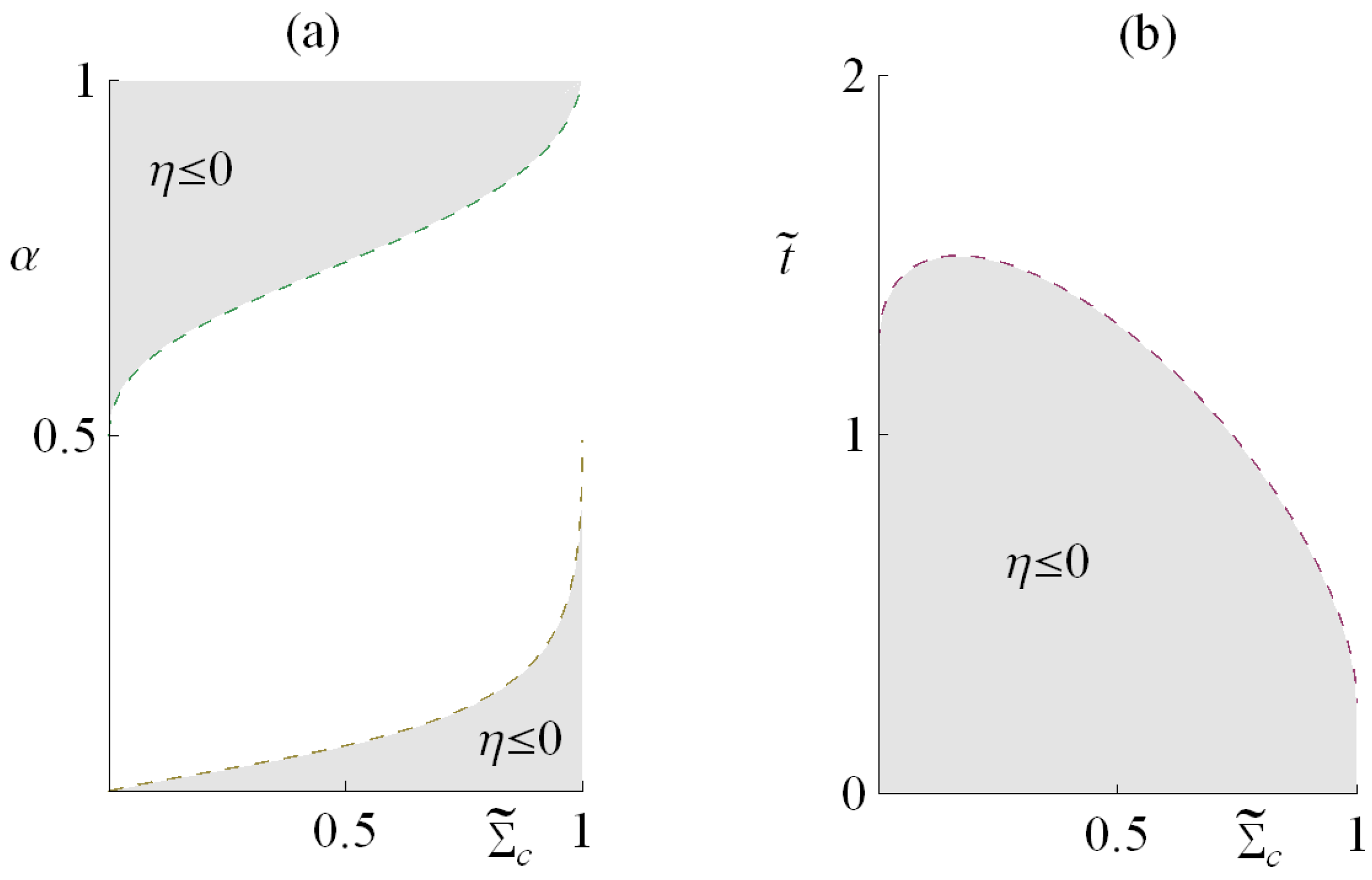
By comparing the entropy production of the low dissipation model and the Carnot-like model, we proposed a connection between the variables that describe each model. We show that, for an HE, the region of physical interest is independent from the operation regime, being equivalent to that for a maximum power LD-HE. That is, defines the acceptable values, and those of (gray shaded areas in Figure 7a,b, respectively). These considerations on the LD model are recovered from physical considerations on the Carnot-like HE. Thus, the difference in the performance of the HEs is not due to the physical configurations of the system, but it comes from the approximations that these models rely on: one over the entropy and the other over the heat fluxes.
We show that the heat leak disappears when fixing the partial contact time in the LD engine, leading to typical endoreversible open parabolic power vs. efficiency curves. However, the connection between the endoreversible case and the LD model is exact only for heat transfer laws with exponents and , and a good approximation in the region . On the other hand, the presence of a heat leak fixes the total operation time and the partial contact time is not constrained, thus, allowing the heat leak to act as an additional degree of freedom (the same efficiency is achieved with different combinations of partial contact time ratios and heat leaks). The reversible limit is not accessible in this case, a maximum operation time is established, and when the heat leak dissipation effects are important, the efficiency may be zero, which is the origin of the loop behavior of the irreversible vs. curves. The connection in the case with heat leak is more complex and its validity depends on the value of .
Acknowledgments
Julian Gonzalez-Ayala acknowledges CONACYT-MÉXICO; José Miguel M. Roco, Alejandro Medina and Antonio Calvo-Hernández acknowledge the Ministerio de Economía y Competitividad (MINECO) of Spain for financial support under Grant ENE2013-40644-R.
Author Contributions
José Miguel M. Roco and Antonio Calvo Hernández conceived and made some simulations of the thermodynamic models. Julian Gonzalez-Ayala and Alejandro Medina. complemented calculations, simulations and the elaboration of graphics. Julian Gonzalez-Ayala and Antonio Calvo Hernández wrote the paper. All authors have read and approved the final manuscript. All authors have read and approved the final manuscript.
Conflicts of Interest
The authors declare no conflict of interest.
References
- Curzon, F.L.; Ahlborn, B. Efficiency of a Carnot Engine at Maximum Power Output. Am. J. Phys. 1975, 43, 22–24. [Google Scholar] [CrossRef]
- Vaudrey, A.; Lanzetta, F.; Feidt, M. H. B. Reitlinger and the origins of the Efficiency at Maximum Power formula for Heat Engines. J. Non-Equilib. Thermodyn. 2014, 39, 199–203. [Google Scholar] [CrossRef]
- Calvo Hernández, A.; Roco, J.M.M.; Medina, A.; Velasco, S.; Guzmán-Vargas, L. The maximum power efficiency 1-root tau: Research, education, and bibliometric relevance. Eur. Phys. J. Spec. Topics 2015, 224, 809–821. [Google Scholar] [CrossRef]
- Arias-Hernandez, L.A.; Angulo-Brown, F.; Paez-Hernandez, R.T. First-order irreversible thermodynamic approach to a simple energy converter. Phys. Rev. E 2008, 77, 011123. [Google Scholar] [CrossRef] [PubMed]
- Izumida, Y.; Okuda, K. Efficiency at maximum power of minimally nonlinear irreversible heat engines. Europhys. Lett. 2012, 97, 10004. [Google Scholar] [CrossRef]
- Apertet, Y.; Ouerdane, H.; Goupil, C.; Lecoeur, P. Irreversibilities and efficiency at maximum power of heat engines: The illustrative case of a thermoelectric generator. Phys. Rev. E 2012, 85, 031116. [Google Scholar] [CrossRef] [PubMed]
- Wang, Y.; Tu, Z.C. Efficiency at maximum power output of linear irreversible Carnot-like heat engines. Phys. Rev. E 2012, 85, 011127. [Google Scholar] [CrossRef] [PubMed]
- Apertet, Y.; Ouerdane, H.; Goupil, C.; Lecoeur, P. Efficiency at maximum power of thermally coupled heat engines. Phys. Rev. E 2012, 85, 041144. [Google Scholar] [CrossRef] [PubMed]
- Gonzalez-Ayala, J.; Arias-Hernandez, L.A.; Angulo-Brown, F. Connection between maximum-work and maximum-power thermal cycles. Phys. Rev. E 2013, 88, 052142. [Google Scholar] [CrossRef] [PubMed]
- Sheng, S.; Tu, Z.C. Universality of energy conversion efficiency for optimal tight-coupling heat engines and refrigerators. J. Phys. A Math. Theor. 2013, 46, 402001. [Google Scholar] [CrossRef]
- Aneja, P.; Katyayan, H.; Johal, R.S. Optimal engine performance using inference for non-identical finite source and sink. Mod. Phys. Lett. B 2015, 29, 1550217. [Google Scholar] [CrossRef]
- Sheng, S.Q.; Tu, Z.C. Constitutive relation for nonlinear response and universality of efficiency at maximum power for tight-coupling heat engines. Phys. Rev. E 2015, 91, 022136. [Google Scholar] [CrossRef] [PubMed]
- Cleuren, B.; Rutten, B.; van den Broeck, C. Universality of efficiency at maximum power: Macroscopic manifestation of microscopic constraints. Eur. Phys. J. Spec. Topics 2015, 224, 879–889. [Google Scholar] [CrossRef]
- Izumida, Y.; Okuda, K. Linear irreversible heat engines based on the local equilibrium assumptions. New J. Phys. 2015, 17, 085011. [Google Scholar] [CrossRef]
- Long, R.; Liu, W. Efficiency and its bounds of minimally nonlinear irreversible heat engines at arbitrary power. Phys. Rev. E 2016, 94, 052114. [Google Scholar] [CrossRef] [PubMed]
- Wang, Y. Optimizing work output for finite-sized heat reservoirs: Beyond linear response. Phys. Rev. E 2016, 93, 012120. [Google Scholar] [CrossRef] [PubMed]
- Schmiedl, T.; Seifert, U. Optimal Finite-Time Processes in Stochastic Thermodynamics. Phys. Rev. Lett. 2007, 98, 108301. [Google Scholar] [CrossRef] [PubMed]
- Tu, Z.C. Efficiency at maximum power of Feynman’s ratchet as a heat engine. J. Phys. A Math. Theor. 2008, 41, 312003. [Google Scholar] [CrossRef]
- Schmiedl, T.; Seifert, U. Efficiency at maximum power: An analytically solvable model for stochastic heat engines. Europhys. Lett. 2008, 81, 20003. [Google Scholar] [CrossRef]
- Schmiedl, T.; Seifert, U. Efficiency of molecular motors at maximum power. Europhys. Lett. 2008, 83, 30005. [Google Scholar] [CrossRef]
- Esposito, M.; Lindenberg, K.; van den Broeck, C. Universality of Efficiency at Maximum Power. Phys. Rev. Lett. 2009, 102, 130602. [Google Scholar] [CrossRef] [PubMed]
- Esposito, M.; Lindenberg, K.; van den Broeck, C. Thermoelectric efficiency at maximum power in a quantum dot. Europhys. Lett. 2009, 85, 60010. [Google Scholar] [CrossRef]
- Golubeva, N.; Imparato, A. Efficiency at Maximum Power of Interacting Molecular Machines. Phys. Rev. Lett. 2012, 109, 190602. [Google Scholar] [CrossRef] [PubMed]
- Wang, R.; Wang, J.; He, J.; Ma, Y. Efficiency at maximum power of a heat engine working with a two-level atomic system. Phys. Rev. E 2013, 87, 042119. [Google Scholar] [CrossRef] [PubMed]
- Uzdin, R.; Kosloff, R. Universal features in the efficiency at maximum work of hot quantum Otto engines. Europhys. Lett. 2014, 108, 40001. [Google Scholar] [CrossRef]
- Curto-Risso, P.L.; Medina, A.; Calvo Hernández, A. Theoretical and simulated models for an irreversible Otto cycle. J. Appl. Phys. 2008, 104, 094911. [Google Scholar] [CrossRef]
- Curto-Risso, P.L.; Medina, A.; Calvo Hernández, A. Optimizing the operation of a spark ignition engine: Simulation and theoretical tools. J. Appl. Phys. 2009, 105, 094904. [Google Scholar] [CrossRef]
- Correa, L.A.; Palao, J.P.; Alonso, D. Internal dissipation and heat leaks in quantum thermodynamic cycles. Phys. Rev. E 2015, 92, 032136. [Google Scholar] [CrossRef] [PubMed]
- Sánchez-Salas, N.; López-Palacios, L.; Velasco, S.; Calvo Hernández, A. Optimization criteria, bounds, and efficiencies of heat engines. Phys. Rev. E 2010, 82, 051101. [Google Scholar] [CrossRef] [PubMed]
- Zhang, Y.; Huang, C.; Lin, G.; Chen, J. Universality of efficiency at unified trade-off optimization. Phys. Rev. E 2016, 93, 032152. [Google Scholar] [CrossRef] [PubMed]
- Iyyappan, I.; Ponmurugan, M. Thermoelectric energy converters under a trade-off figure of merit with broken time-reversal symmetry. arXiv 2016. [Google Scholar]
- Angulo-Brown, F. An ecological optimization criterion for finite-time heat engines. J. Appl. Phys. 1991, 69, 7465–7469. [Google Scholar] [CrossRef]
- Arias-Hernández, L.A.; Angulo-Brown, F. A general property of endoreversible thermal engines. J. Appl. Phys. 1997, 81, 2973–2979. [Google Scholar] [CrossRef]
- Long, R.; Li, B.; Liu, Z.; Liu, W. Ecological analysis of a thermally regenerative electrochemical cycle. Energy 2016, 107, 95–102. [Google Scholar] [CrossRef]
- Esposito, M.; Kawai, R.; Lindenberg, K.; van den Broeck, C. Efficiency at Maximum Power of Low-Dissipation Carnot Engines. Phys. Rev. Lett. 2010, 105, 150603. [Google Scholar] [CrossRef] [PubMed]
- De Tomás, C.; Roco, J.M.M.; Calvo Hernández, A.; Wang, Y.; Tu, Z.C. Low-dissipation heat devices: Unified trade-off optimization and bounds. Phys. Rev. E 2013, 87, 012105. [Google Scholar] [CrossRef] [PubMed]
- Holubec, V.; Ryabov, A. Efficiency at and near maximum power of low-dissipation heat engines. Phys. Rev. E 2015, 92, 052125. [Google Scholar] [CrossRef] [PubMed]
- Holubec, V.; Ryabov, A. Erratum: Efficiency at and near maximum power of low-dissipation heat engines. Phys. Rev. E 2015, 93, 059904. [Google Scholar] [CrossRef] [PubMed]
- Holubec, V.; Ryabov, A. Maximum effciency of low-dissipation heat engines at arbitrary power. J. Stat. Mech. 2016, 2016, 073204. [Google Scholar] [CrossRef]
- Calvo Hernández, A.; Medina, A.; Roco, J.M.M. Time, entropy generation, and optimization in low-dissipation heat devices. New J. Phys. 2015, 17, 075011. [Google Scholar] [CrossRef]
- Gonzalez-Ayala, J.; Calvo Hernández, A.; Roco, J.M.M. Irreversible and endoreversible behaviors of the LD-model for heat devices: The role of the time constraints and symmetries on the performance at maximum χ figure of merit. J. Stat. Mech. 2016, 2016, 073202. [Google Scholar] [CrossRef]
- Gonzalez-Ayala, J.; Calvo Hernández, A.; Roco, J.M.M. From maximum power to a trade-off optimization of low-dissipation heat engines: Influence of control parameters and the role of entropy generation. Phys. Rev. E 2017, 95, 022131. [Google Scholar] [CrossRef] [PubMed]
- Hu, Y.; Wu, F.; Ma, Y.; He, J.; Wang, J.; Calvo Hernández, A.; Roco, J.M.M. Coefficient of performance for a low-dissipation Carnot-like refrigerator with nonadiabatic dissipation. Phys. Rev. E 2013, 88, 062115. [Google Scholar] [CrossRef] [PubMed]
Figure 1.
(a) Sketch of a low dissipation heat engine characterized by entropy generation laws and ; (b) Sketch of an irreversible Carnot-like heat engine characterized by generic heat transfers , and .
Figure 1.
(a) Sketch of a low dissipation heat engine characterized by entropy generation laws and ; (b) Sketch of an irreversible Carnot-like heat engine characterized by generic heat transfers , and .
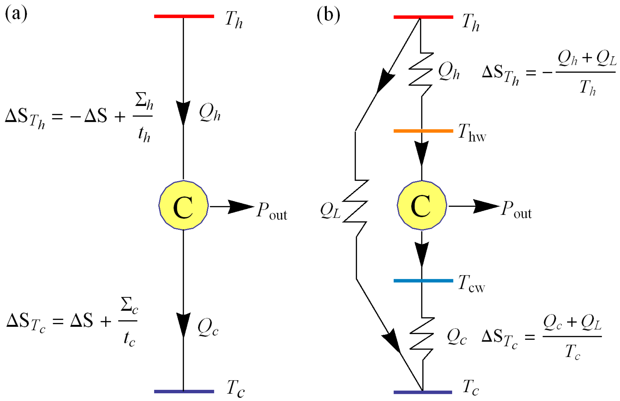
Figure 2.
(a) and from Equation (9). Note how, as the heat leak increases, the possible physical combinations of and become more limited; (b) according to Equation (10). The representative values , have been used, however, the displayed behavior is similar for any other combination of values.
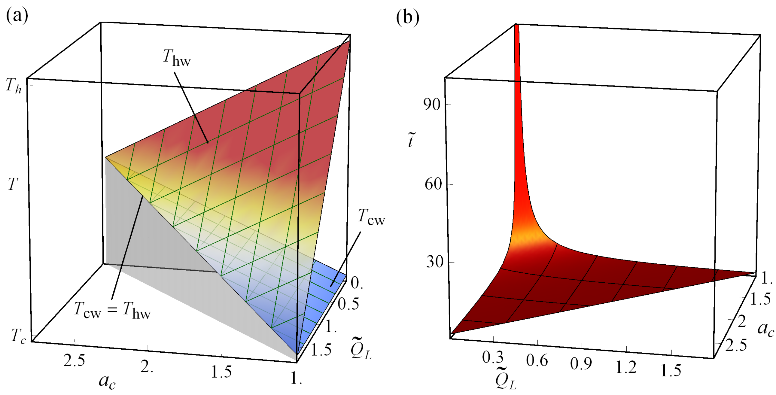
Figure 3.
Possible values of as a function of the control parameters and . We used the values and .
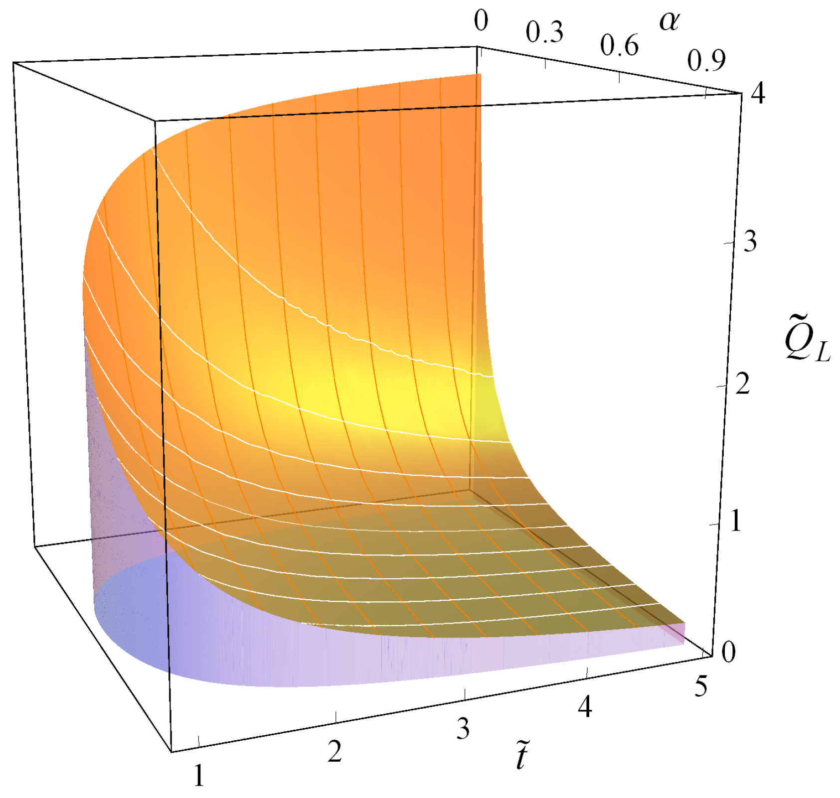
Figure 4.
(a) upper and lower bounds of the MP efficiency in terms of the exponent of the heat transfer law k of the Carnot-like heat engine; (b) the values that reproduce the upper and lower bounds of the endoreversible engine.
Figure 4.
(a) upper and lower bounds of the MP efficiency in terms of the exponent of the heat transfer law k of the Carnot-like heat engine; (b) the values that reproduce the upper and lower bounds of the endoreversible engine.

Figure 5.
Maximum-power efficiency for the symmetric case , assuming the LD condition that and using the resulting value that fulfills the endoreversible hypothesis. Notice that the matching with the CA efficiency is approximate for the interval and is exact for , as can be seen in the zoom of this region on the right side of the figure.

Figure 6.
Influence of the heat leak over the optimized efficiencies appearing in Figure 4. See the text for explanation.
Figure 6.
Influence of the heat leak over the optimized efficiencies appearing in Figure 4. See the text for explanation.
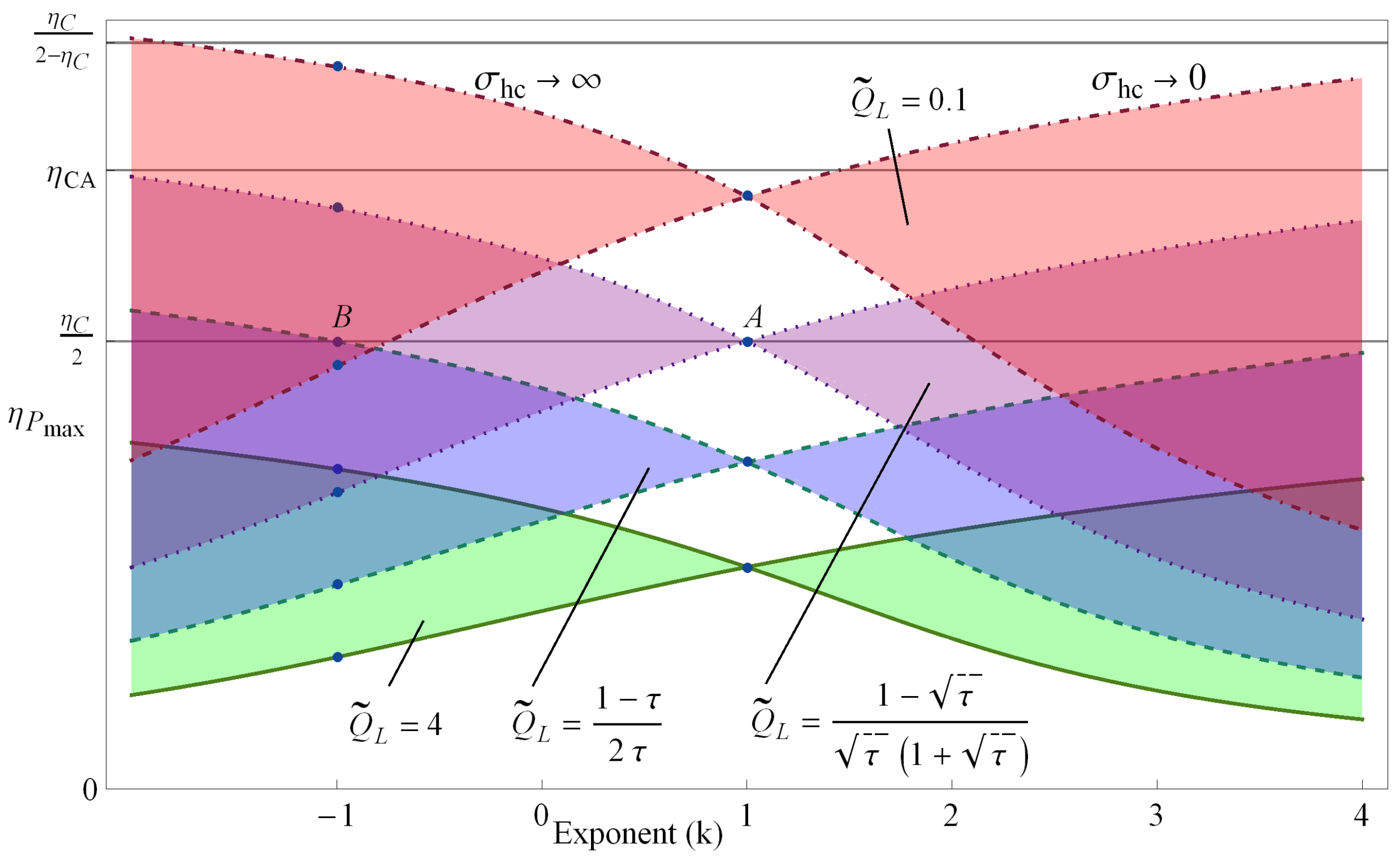
Figure 7.
(a) Physically well behaved region of the ‒ variables. The shaded areas come from the LD model and the dashed curves come from the Carnot-like model; (b) The same for the ‒ variables. Notice the agreement in both models. In these plots, we use .
Figure 7.
(a) Physically well behaved region of the ‒ variables. The shaded areas come from the LD model and the dashed curves come from the Carnot-like model; (b) The same for the ‒ variables. Notice the agreement in both models. In these plots, we use .
© 2017 by the authors. Licensee MDPI, Basel, Switzerland. This article is an open access article distributed under the terms and conditions of the Creative Commons Attribution (CC BY) license (http://creativecommons.org/licenses/by/4.0/).
Share and Cite
MDPI and ACS Style
Gonzalez-Ayala, J.; Roco, J.M.M.; Medina, A.; Calvo Hernández, A. Carnot-Like Heat Engines Versus Low-Dissipation Models. Entropy 2017, 19, 182. https://doi.org/10.3390/e19040182
AMA Style
Gonzalez-Ayala J, Roco JMM, Medina A, Calvo Hernández A. Carnot-Like Heat Engines Versus Low-Dissipation Models. Entropy. 2017; 19(4):182. https://doi.org/10.3390/e19040182
Chicago/Turabian StyleGonzalez-Ayala, Julian, José Miguel M. Roco, Alejandro Medina, and Antonio Calvo Hernández. 2017. "Carnot-Like Heat Engines Versus Low-Dissipation Models" Entropy 19, no. 4: 182. https://doi.org/10.3390/e19040182
Note that from the first issue of 2016, this journal uses article numbers instead of page numbers. See further details here.