Face Verification with Multi-Task and Multi-Scale Feature Fusion

Abstract

Face verification for unrestricted faces in the wild is a challenging task. This paper proposes a method based on two deep convolutional neural networks (CNN) for face verification. In this work, we explore using identification signals to supervise one CNN and the combination of semi-verification and identification to train the other one. In order to estimate semi-verification loss at a low computation cost, a circle, which is composed of all faces, is used for selecting face pairs from pairwise samples. In the process of face normalization, we propose using different landmarks of faces to solve the problems caused by poses. In addition, the final face representation is formed by the concatenating feature of each deep CNN after principal component analysis (PCA) reduction. Furthermore, each feature is a combination of multi-scale representations through making use of auxiliary classifiers. For the final verification, we only adopt the face representation of one region and one resolution of a face jointing Joint Bayesian classifier. Experiments show that our method can extract effective face representation with a small training dataset and our algorithm achieves 99.71% verification accuracy on Labeled Faces in the Wild (LFW) dataset.

1. Introduction

With the convolution neural network, in recent years, the vision community has made great progress in many challenge problems, such as object detection [1], semantic segmentation [2], object classifiaction [3] and so on. At the same time, face verification methods based on deep convolutional neural networks (CNNs) have achieved high performance [4,5,6,7]. As it does not require too much user cooperation, compared to iris verification, fingerprint verification and other methods, face verification has a better user experience. Thus, face verification recently has attracted more and more concern. In general, using a convolution neural network to do face verification needs the following steps: a pair of face images is taken as input into the convolution neural network for feature extraction, and then the extracted two features are sent to the classifier to calculate the similarity, according to the relationship between similarity and the threshold, judging whether it is the face of the same person. Face representation learning plays an important role in face recognition. Some researchers combine deep face representation and verification into one system, which is learning to map faces into similarity space directly [4]. However, it is much harder to learn the mapping in terms of a lack of training data. In this paper, we use the deep CNN as a feature extractor and adopt an extra classifier to make face representation more discriminative as in [5,6,7].

The common convolution neural network for object classification such as Alexnet [3], VGG [8], GoogleNet [9], Residual net [10], only use the softmax loss function for multi-class classification. During inference, the input is directly classified by the convolution neural network. However, different from object classification, face verification not only needs to have the ability to distinguish different identities, but also needs to make the distance of the same identity small enough. The network only trained by softmax loss function can not make intra-class closer. Siamese nets [11] use a pair of images as input and directly output the similarity of the images. Though Siamese nets pay attention to the distance between two samples, the separation of the different classes is ignored. DeepID2 [6] adds a verification loss to softmax loss function, which is called contrastive loss, and solves the problem of ignoring the separation of different classes. FaceNet [4] uses triplet loss to obtain the same purpose. Triplet loss utilizes the distance relationship between anchor, positive, and negative, minimizes the distance between anchor and positive, and maximizes the distance between anchor and negative. Contrastive loss and triplet loss need to pair the training samples, and there are no reasonable ways to pair samples efficiently for now. Some work uses online search to get the hard examples to pair. This makes it necessary to perform a work of selecting training samples before each iteration thus increasing the training time. In this paper, we design two CNNs to extract face features that can have strong abilities of identification and verification. CNN1, which is only supervised by an identification signal, is designed for setting different identities apart. In addition, CNN2 is supervised by the combination of identification and semi-verification signals, which can make the distance of the same person small enough. Semi-verification is inspired by triplet loss in Facenet and verification signal in DeepID2, which represents the distance of pairs from the same identity. Different with the DeepID2 and Facenet, we do not need to select the training samples before each iteration, which avoids the extra time consumption. We have similar thoughts to center loss [12], which is making intra-class samples as close as possible. Center loss calculates the distance between samples and their classes’ centers to minimize the intra-class variations. During backward propagation, center loss needs to update class centers, which means that the extra calculation or parameters, though not complex, are needed. Our method does not need any extra parameters and reduces the intra-class variations that softmax loss function can not solve.

In face pre-processing, it is hard to do great normalization for faces with variation caused by poses. In [13], Li proposes using the distance of landmarks instead of eye centers for face normalization, which is said to be relatively invariant to pose variations in yaw poses. In our system, we combine this method and use the eye centers method to do face normalization in a certain condition.

Inspired by [9,14], we add auxiliary classifiers to assist the training of CNN. In addition, these auxiliary classifiers provide multi-scale features for recognition. Thus, a stronger feature can be obtained by concatenating these multi-scale features. Recently, most face verification methods catenate face representations of multi-resolutions and multi-regions based on deep CNNs to construct a feature with high dimension [6,7]. This will conduct high computation and a large burden of storage. In our work, we combine the face representations of two networks and obtain a compact feature as the final face representation. For each network, only one resolution and one region of a face are used. Due to the final feature combining the multi-scale features coming from two CNNs trained by different signals, we called it multi-task and multi-scale features fusion.

The overall framework of our face verification method is illustrated in Figure 1. In addition, our effective face representation joint Joint Bayesian classifier achieves high performance (99.71%) on the LFW dataset with a small training database.

The rest of this paper is constructed as follows: we introduce the semi-verification signal in Section 2, which is used for supervising the training of one deep CNN. In Section 3, we present two deep CNNs and the training algorithm. Face verification based on the proposed framework will be presented in Section 4. In Section 5, we present the performance of our method compared with others based on deep CNN. Conclusions will be drawn in Section 6.

2. The Proposed Loss Function

Recently, there have been a lot of methods to add the verification information to the CNN for face verification tasks, such as contrastive loss [6], triplet loss [4], and lifted structured embedding [15]. The CNN trained with verification information can adjust the parameters end-to-end, so that the features generated from these CNN have greater discriminant power than those from normal networks that only use the cross entropy loss. However, contrastive loss [6] and triplet loss [4] need to pair the training sample. Contrastive loss [6] requires not only the positive pairs, but also negative pairs (where the positive pair refers to two different face images having the same identity, and the negative pair refers to two different face images having different identities). However, the number of positive pairs and the number of negative pairs are extremely unbalanced. For a dataset containing n individuals and m face images per person, the number of positive pairs is $n\left(\genfrac{}{}{0pt}{}{m}{2}\right)$, and the number of negative pairs is $m^2\left(\genfrac{}{}{0pt}{}{n}{2}\right)$. When $m\ll n$, $n\left(\genfrac{}{}{0pt}{}{m}{2}\right)\ll m^2\left(\genfrac{}{}{0pt}{}{n}{2}\right)$, which means that the number of negative pairs is much larger than the number of positive pairs. Therefore, unreasonable pairing can not improve the performance or even worse. Triplet loss [4] proposed online and offline methods for selecting training pairs, and each anchor uses a semi-hard sample as its corresponding negative sample. Although lifted structured embedding [15] does not need to pair the samples in a complex method, if the batchsize is N, a high cost $O\left(N^2\right)$ is entailed. The research community still does not have reasonable ways to pair samples.

In order to solve the above problems, we propose a semi-verification signal and a corresponding pair selection method so that the verification information can be added to the CNN reasonably and efficiently.

The semi-verification signal means that only the pairs of the same identity will be used to compute verification loss. It minimizes the L2-distance between the face images of the same identity:

$$Semi-verificationSignal=\frac{1}{\mid S\mid }\sum _{(i,j)\in S}\parallel f_i-f_j{\parallel }_2^2,$$

(1)

where S is an index set of face pairs belonging to the same identity. It does not contain pairs of different identities, which is different from verification signals. The negative pairs do not need to be selected, and the imbalance between positive and negative pairs talked above exists no more. In addition, it is the reason why we call it a semi-verification signal. Reducing the intra-class variations and keeping the separable inter-class differences unchanged can also achieve the same purpose as the contrastive loss [6].

Supposing that there are n different face images from one person, it will be $\left(\genfrac{}{}{0pt}{}{n}{2}\right)$ positive pairs. In this view, we only want to use a part of these pairs. However, randomly selected sample pairs cannot establish close relationships between all samples.

Suppose that we randomly select m pairs from $\left(\genfrac{}{}{0pt}{}{n}{2}\right)$ pairwise combination and there will be such a situation that some images do not appear in selected pairs any more. As shown in Figure 2, it will make images of this person be divided into two clusters after training. As a result, the distance between m pairs of face images is small enough in one cluster, but in the other one will not. In addition, the distance between two clusters will not be small enough.

For the purpose of solving the problems mentioned above, we institute positive pairs by creating a circle as a pair selection method. Supposing that there are N training samples of class i in the training data set, we number these samples $1,2,···,N$. CNN extracts features $f_j(j=1,2,···,N)$ for these N samples. As shown in Figure 3, one feature corresponding to one image is connected with its directly connected neighbors, and there are no extra connections between it and other features. In other words, $f_j$ only pairs with $f_{j-1}$ or $f_{j+1}$. We can easily solve the problem above in this way. On the one hand, it reduces the computation cost to a certain extent $O\left(N\right)$. On the other hand, it establishes direct or indirect relationships between all face images.

In order to make the facial features extracted by CNN have strong identification and verification performance, two kinds of loss functions are used in this paper. One is identification loss, and the other is joint identification and semi-verification loss:

$$IdentificationLoss=-\sum _{i=1}^n-p_{i}log{\widehat{p}}_i,$$

(2)

where $p_i$ is the target probability distribution, and ${\widehat{p}}_i$ is the predicted probability distribution. If t is the target class, then $p_t=1$, and $p_j=0$ for $j\ne t$.

The joint identification and semi-verification loss can be formulated as follows:

$$JointLoss=-\sum _{i=1}^n-p_{i}log{\widehat{p}}_i+\frac{\lambda }{2\mid S\mid }\sum _{(i,j)\in S}\parallel f_i-f_j{\parallel }_2^2,$$

(3)

where $-{\sum }_{i=1}^n-p_{i}log{\widehat{p}}_i$ represents the identification part, and $\parallel f_i-f_j{\parallel }_2^2$ denotes a semi-verification signal. S is a index set of face pairs belonging to the same identity, and $\lambda$ is a hyper-parameter used to balance the contributions of two signals.

3. The CNN Architecture and Detailed Parameters

Our face representation is a combination of features from two deep convolutional neural networks. The first CNN (CNN1) is supervised by identification signal only and the second one (CNN2) is supervised by joint identification and semi-verification signals.

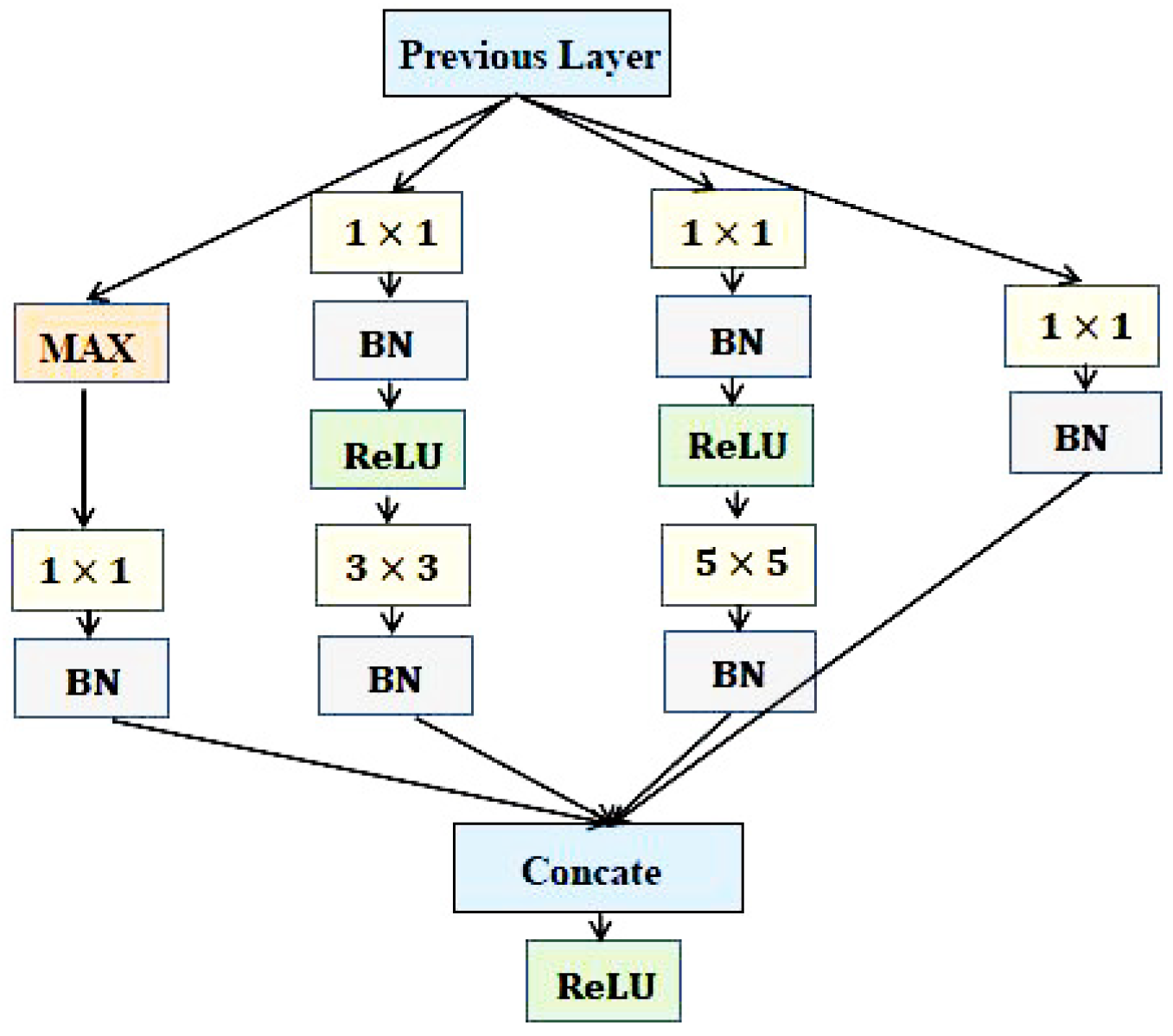
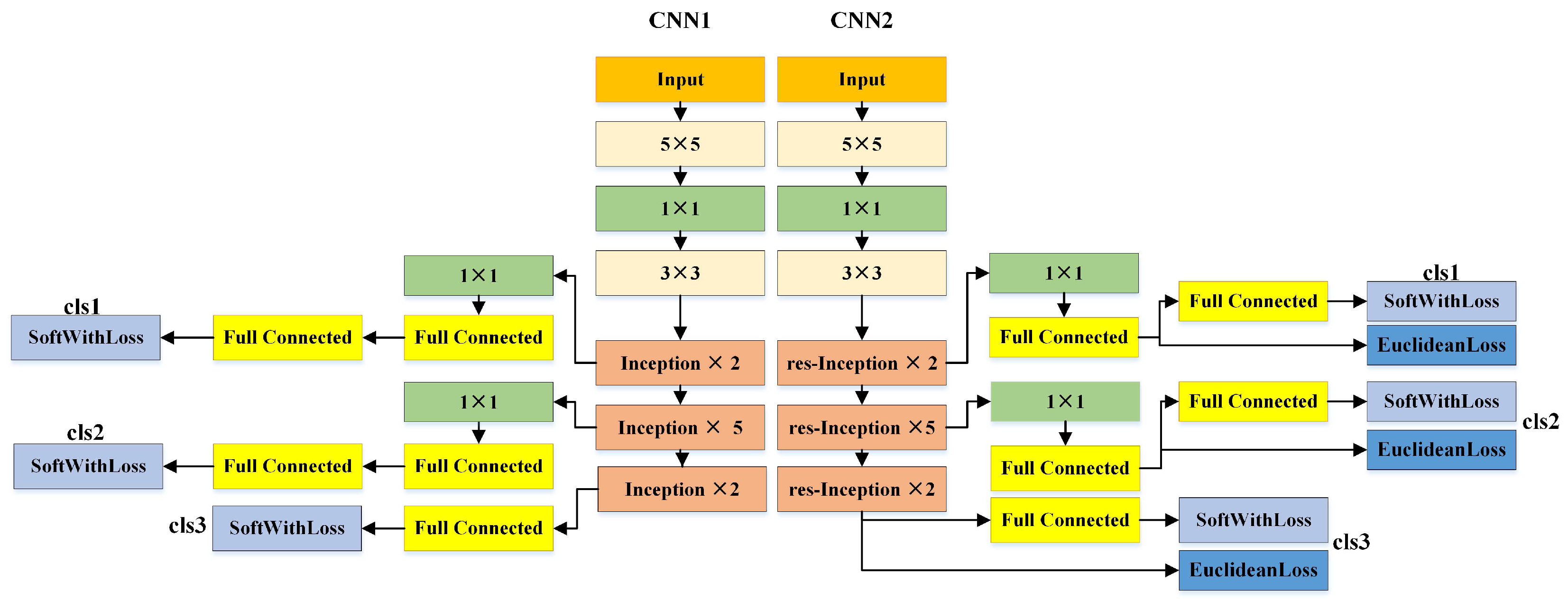
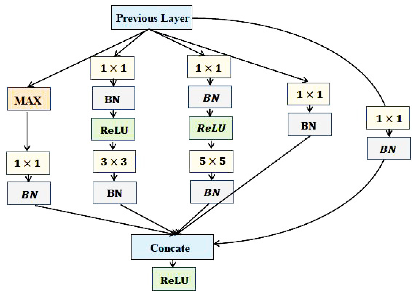
3.1. Deep CNNs for Face Representation

Our deep CNNs contains two CNNs. CNN1 is constructed by ordinary convolution in shallow layers and Inception architecture in deep layers. Inception can be traced back to GoogleNet [9], and it is used for solving the problem of the increase of high computation cost in the process of making a deeper network. It can not only increase the depth and width of convolution neural network at a certain computation cost, but also extract multi-scale features for face representation. The framework of Inception used in CNN1 is shown in Figure 4.

As shown in Figure 4, we concatenate different sizes of convolutional layers $(1\times 1,3\times 3,5\times 5)$ and Max-Pooling in one layer. A small size of convolutional layer can focus more on local information, and a larger one focuses on the global. It is the reason why Inception can extract multi-scale features. In addition, $1\times 1$ reduction is used before $3\times 3$ and $5\times 5$, and we also adopt Batch Normalization (BN) [16] after each convolution. BN can help our algorithm to coverage at a high speed and mitigate the problem of overfitting.

When it comes to the activation function, we explore using ReLU [17] after BN for each convolution in Inception. In addition, for the output of Inception, which concatenates the results of multi-scale convolution, we adopt ReLU after concatenating layer. In this way, information can propagate more from the former layers to the later and the back propagation is more smooth [18]. The overall framework of CNN1 can be seen in Figure 5.

One difference between CNN1 and CNN2 in architecture is that we explore using extra residual networks in CNN2, which is similar to [18]. Residual network [10] is not only used for ordinary convolution but also for Inception, which is called res-Inception. The framework of res-Inception is shown in Figure 6. The reason why we want to introduce a residual network in CNN2 is that it can make information propagation much smoother from the former to the latter.

It also mitigates the problems of overfitting and low speed of coverage in the training process. The overall framework of CNN2 is shown in Figure 5.

The deepening of the network will mostly cause a vanishing gradient. Although a residual network has been introduced, the difficulty of training CNNs is still a problem. Inspired by [9,14], we explore two auxiliary classifiers in both deep CNNs as shown in Figure 5. We call them cls1 and cls2. For consistency, the original classifier is called cls3. Recently, much research has discovered that the features from intermediary layers have great complement power with features from the top layer. In our work, each cls used for classification has a fully connected layer and loss layer, so we can get three features for each CNN. The three features produced from different layers correspond to different scales. In order to extract multi-scale face representation features, the final face representation of each CNN is formed by concatenating these three features. From this, we obtain local information from the former layers and the global information from the latter layers. As we can see in Section 5.2, concatenating features from different layers will achieve a greater improvement than using just one feature.

3.2. Detailed Parameters for NNs and the Training Algorithm

The detailed parameters of CNN1 and CNN2 are shown in

Table 1. The detailed parameters of convolution and Max-Pooling layers; (“#” stands for the number of corresponding filters in the layer).

Type	Size/Stride	Channel	$\#1\times 1$	$\#3\times 3$ Reduction	$\#3\times 3$	$\#5\times 5$ Reduction	$\#5\times 5$	Residual Network	#Pooling Reduction
Conv	$5\times 5/1$	64	-	-	-	-	-	-	-
Pooling	$3\times 3/2$	-	-	-	-	-	-	-	-
Conv	$1\times 1/1$	64	-	-	-	-	-	92	-
Conv	$3\times 3/1$	92	-	-	-	-	-		-	-
Pooling	$3\times 3/2$	-	-	-	-	-	-	-	-
res-Incep	-	256	64	96	128	16	32	256	32
res-Incep	-	480	128	128	192	32	96	480	64
cls1 Pooling	$5\times 5/3$	-	-	-	-	-	-	-	-
cls1 Conv	$1\times 1/1$	128	-	-	-	-	-	-	-
cls1 FC	-	512	-	-	-	-	-	-	-
cls1 FC	-	$15,340$	-	-	-	-	-	-	-
cls1 softmax	-	$15,340$	-	-	-	-	-	-	-
Pooling	$3\times 3/2$	-	-	-	-	-	-	-	-
res-Incep	-	512	192	96	208	16	48	512	64
res-Incep	-	512	160	112	224	24	64	512	64
res-Incep	-	512	128	128	256	24	64	512	64
res-Incep	-	832	256	160	320	32	128	832	128
res-Incep	-	512	192	96	208	16	48	512	64
cls2 Pooling	$5\times 5/3$	-	-	-	-	-	-	-	-
cls2 Conv	$1\times 1/1$	128	-	-	-	-	-	-	-
cls2 FC	-	512	-	-	-	-	-	-	-
cls2 FC	-	$15,340$	-	-	-	-	-	-	-
cls2 softmax	-	$15,340$	-
Pooling	$3\times 3/2$	-	-	-	-	-	-	-	-
res-Incep	-	832	256	160	320	32	128	832	128
res-Incep	-	1024	384	192	384	48	128	1024	128
Pooling	$6\times 6/6$	-	-	-	-	-	-	-	-
cls3 FC	-	$15,340$	-	-	-	-	-	-	-
cls3 softmax	-	$15,340$	-	-	-	-	-	-	-

. We should point out that there is no usage of residual networks in CNN1, so the parameters of the residual network for CNN1 is none. The training of CNN1 and CNN2 is based on a gradient descent algorithm with different supervisory signals. CNN1 is supervised by an identification signal. The identification signal can make the face representation have a strong ability to distinguish different identities, and this is formulated in Equation (2).

Although CNN supervised by identification can be used for verification, it cannot make the distance of faces from the same identity small enough. Enlarging the distance between different identities and decreasing that of the same are important for face verification tasks. Thus, we use joint identification and semi-verification signals to train CNN2. Unlike verification signals, semi-verification only uses samples from the same identity to compute loss. It can either decrease the distance of the intra-identity. The loss used for CNN2 is formulated in Equation (3). Thus, multi-task information can be obtained by concatenating features that come from CNN1 and CNN2.

For the back propagation process, we compute the partial derivative of loss about parameters $(w,b)$. Then, parameters can be updated through the partial derivative and learning rate $\eta$. Since CNN2 needs to calculate the distance between paired sampled features, we use the following method to construct each batch sample in order to facilitate calculation. Supposing that we have N (N is an even number) samples in a batch, denote these N samples as $1,2,···,N$. We pair the first $N/2$ samples of the batch with the last $N/2$ samples. The sample image $i(i<N/2)$ in the batch belongs to the same person as the $N/2+i$ sample. Therefore, when training CNN2, we slice the features according to the the “batch” dimension and then calculate the distance between pairs. The details of our learning algorithm is shown in Algorithm 1.

Algorithm 1 The learning algorithm of CNN.
Input: Training database $(x_i,y_i),i=1,2,\dots ,n$, where $x_i$ denotes face image and $y_i$ is identity label, $batchsize=32$;
Output: Weight parameters;
1:	while not coverage do
2:	$t=t+1$, sample training set from training database $(x_i,y_i)$, the size of each training set is equal to batch size.;
3:	Compute forward process: $$f_i=Conv(x_i,{\theta }_c)$$
4:	Slice the output of the last convolutional layer at the point $⌊batchsize/2⌋$.
5:	Compute identification loss and verification loss respectively: $$IdentificationLoss=-{\sum }_{i=1}^{batchsize}-p_{i}log{\widehat{p}}_i$$ $$VerificationLoss=\frac{1}{⌊batchsize/2⌋}{\sum }_{i=1}^{⌊batchsize/2⌋}\parallel f_i-f_{i+⌊batchsize/2⌋}{\parallel }_2^2$$
6:	Compute the value of loss function: $$Loss=IdentificationLoss\left(\mathrm{for}\mathrm{CNN}1\right)$$ $$Loss=IdentificationLoss+\lambda VerficationLoss\left(\mathrm{for}\mathrm{CNN}2\right)$$
7:	Compute gradient: $$▽{\theta }_c=\frac{\partial loss}{\partial {\theta }_c}$$
8:	Update network parameters: $${\theta }_c={\theta }_c-\eta \left(t\right)▽{\theta }_c$$
9:	end while

4. Face Verification with Classifier

For face representation, we adopt CNN1 and CNN2 to extract features of normalized faces, respectively. Then, two extracted features are concatenated to be a relatively high dimension feature. The final representation of a face is formed by computing PCA reduction of the catenated feature. After face representation, we explore a classifier to improve the discriminative ability of features.

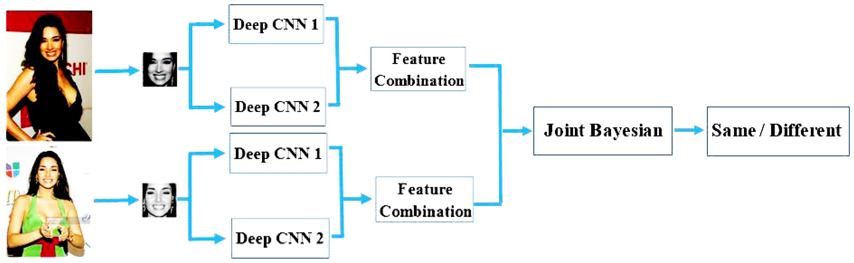
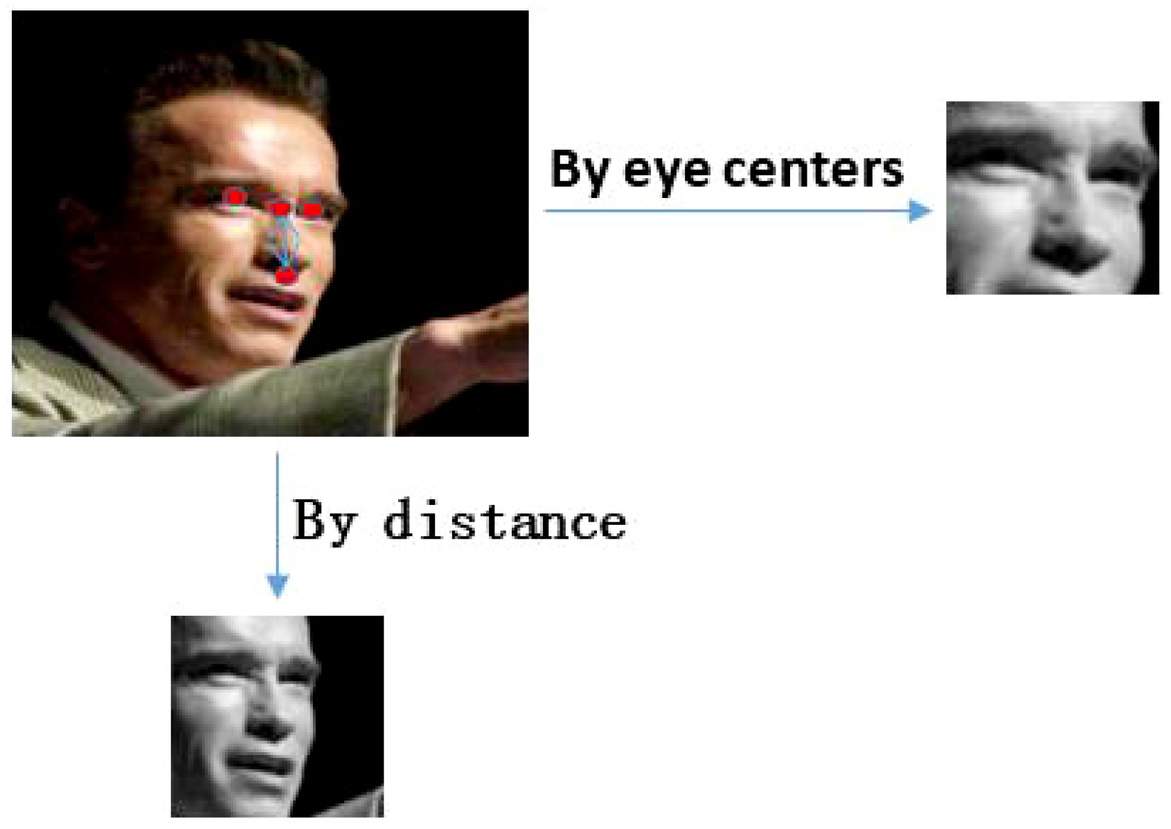
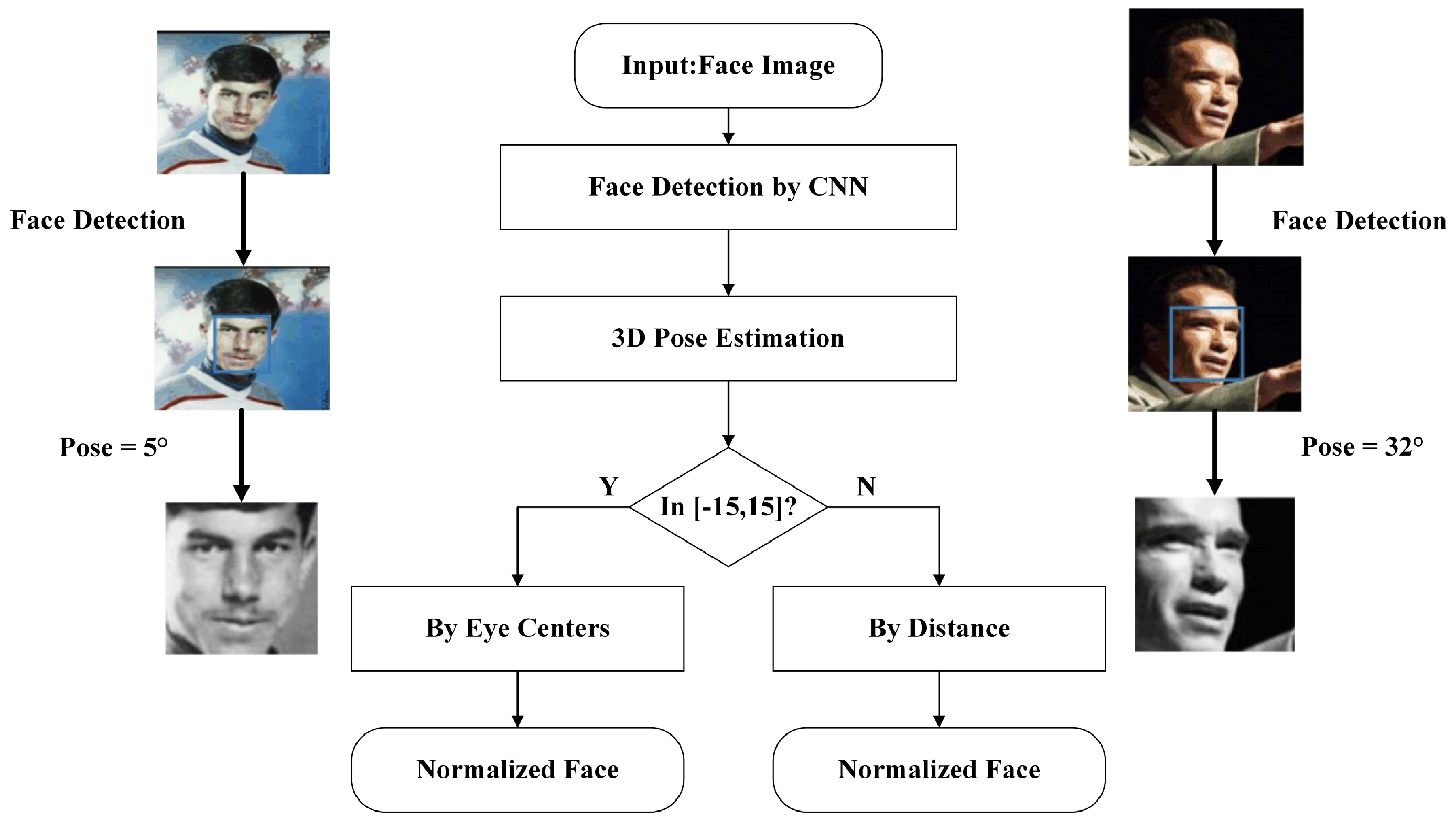
4.1. Face Representation

Identifying faces with different poses is one of the hardest tasks in face verification, especially ones in yaw angles. As shown in Figure 7, compared with ordinary canonical faces, the distance between two eyes is smaller when faces are in yaw angles, and face normalization with eye centers can conduct the results to be just parts of faces especially. It has negative effects for face verification. However, normalization by the distance between two landmarks of the nose is relatively invariant to yaw angles. However, accurate landmarks of the nose are much harder to be detected than eyes.

In order to solve two problems mentioned above, we adopt different methods to deal with face normalization, and the flow of this strategy is described in Figure 8. First of all, an image is detected by a face detector based on CNN [19]. Then, we estimate the pose and locate face landmarks of the detected face through a 3D poses algorithm [20]. For those faces, whose yaw angle belongs to $[-15,15]$, we adopt landmarks of eye centers for normalization. For others, we use the landmarks of eye center and nose for alignment. By this method, it can not only ensure the accuracy of face normalization for faces with small or no pose variance, but also ensure that results of faces with poses in yaw angles containing the whole face regions.

After face pre-processing, we can obtain images that only contain face regions. The normalized face image is taken as the input of two networks, and outputs are concatenated to form the final face representation with PCA reduction.

4.2. Face Verification by Two Classifiers

In order to increase the ability of discriminant of face representation, we explore Cosine Distance and Joint Bayesian [21], respectively. These two classifiers both compute the similarity of a pair of features $f_i$ and $f_j$. That is,

$$CosineDistance=\frac{\langle f_i,f_j\rangle }{\parallel f_i\parallel \parallel f_j\parallel },$$

(4)

$$JointBayesian=-log\frac{p(f_i,f_j|H_I)}{p(f_i,f_j|H_E)}.$$

(5)

According to [21], $H_I$ and $H_E$ in Equation (5) means two hypotheses. The former represents an intra-personal hypothesis in which two features $f_i$ and $f_j$ belong to the same identity and the latter is an extra-personal hypothesis in which two features are from different identities.

5. Experiments

Our experiments are based on Caffe [22], with NVIDIA GT980X GPU with 4 GB of onboard memory, using a single GPU. We train our model on the TesoFaces database, which contains 400,000 face images of 15,340 celebrities from the internet. We collect massive Eastern and Western celebrities’ photos from the internet. Any names appearing in the LFW [23] are removed in order to make it possible to train on this new dataset. For each class, the method claimed in Section 4.1 are used to detect faces. We delete such images that no bounding box exists or the size of the bounding box is too small. After that, we manually delete some other images such as duplicates or bad quality. The final database has 0.4 M images, consisting of 15,340 identities. The faces are cropped and aligned to the size of $100\times 100$ in both training and testing phases. Furthermore, we evaluate our method on LFW [23] and YouTube Faces Database(YTF) [24], which are challenging datasets for face verification in the wild. We do not use LFW or TesoFaces to train Joint Bayesian and PCA. CASIA-Webfaces [13] is used.

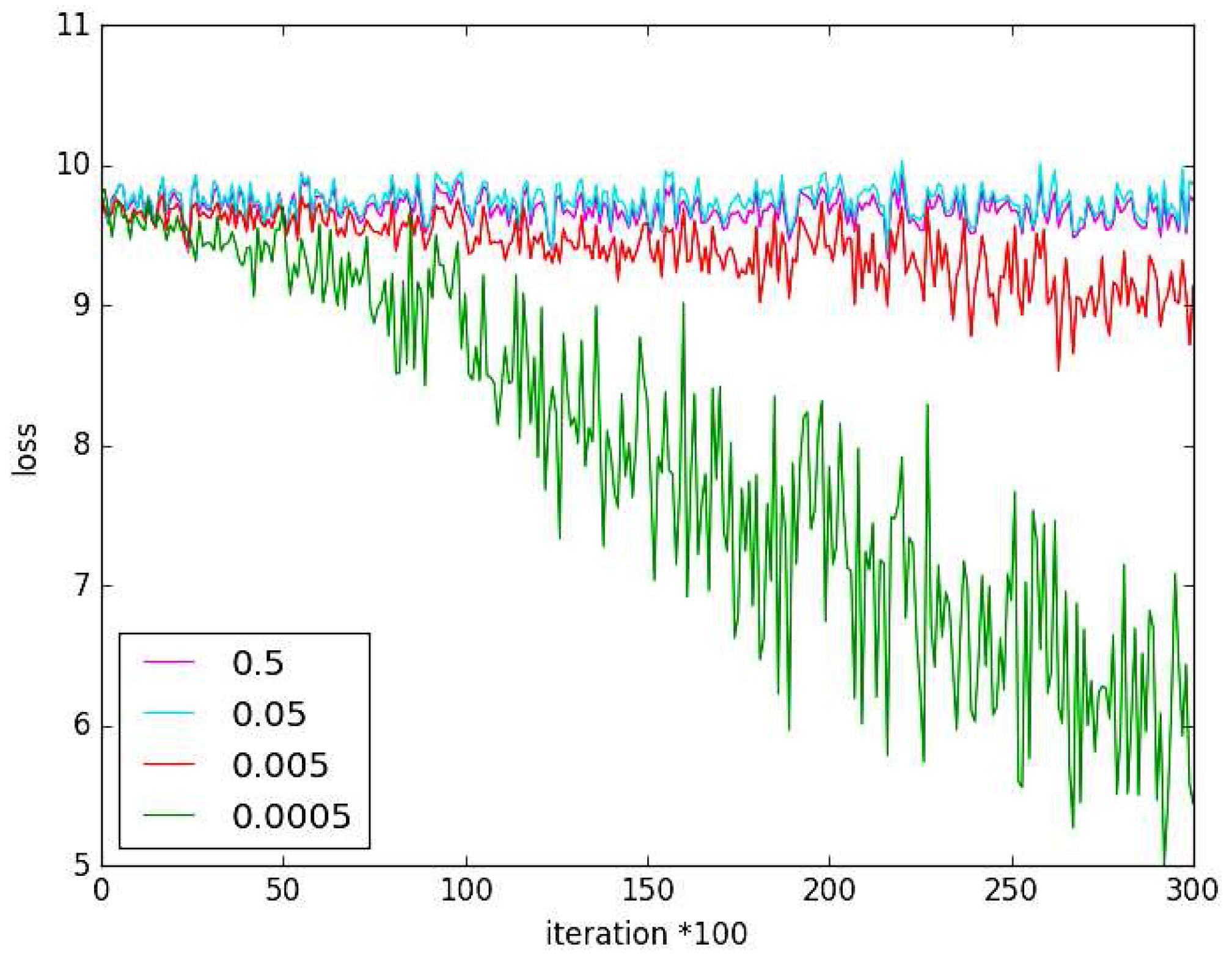
5.1. Experiment on Hyper-Parameter $\lambda$

We research the balance between identification and semi-verification signals by a hyper-parameter $\lambda$. In our experiment, we try to explore five different values of $\lambda (\lambda =0,0.0005,0.005,0.05,0.5)$. With the increase of $\lambda$, the contribution of semi-verification to loss function is much greater. If $\lambda =0$, only identification signals will take effect.

We decide the value of $\lambda$ in two views. In the first view, the decrease of loss function is used for measuring the performance of different values. Furthermore, the second view is to use face verification accuracy on the LFW dataset to determine whether $\lambda$ is zero or not. The TesoFaces database is split into training and validation sets. The proportion of the training sets and validation sets is 7:3. We firstly train our model on the train set of TesoFaces and test on the validation set to show the different performance of different $\lambda$ values. The final model is trained entirely by the TesoFaces database. Figure 9 shows the curve of the decrease of loss with different hyper-parameters. As we can see, the large value of $\lambda =0.5$ and $\lambda =0.05$ cause the loss to not fall any more. Furthermore, the loss of $\lambda =0.005$ decreases very slowly. In contrast to the results of the other three values, the loss of $\lambda =0.0005$ is decreasing at a high speed and will converge finally.

Table 2. Accuracy with different values of $\lambda$ by Cosine Distance.

Signal	Identification ($\mathit{\lambda }=0$)	Identification & Semi-Verification ($\mathit{\lambda }=0.0005$)
Accuracy	97.77%	98.18%

shows the face verification rate on the LFW dataset by Cosine Distance when $\lambda =0$ and $\lambda =0.0005$. We can see that training with the combination of identification and semi-verification, that is, $\lambda =0.0005$, has a good performance. Furthermore, the weight of semi-verification should be a little small. That is to say, the identification signal takes a much more important role in the CNN training process. Furthermore, semi-verification plays the role of regularization to a certain extent.

5.2. Learning Effective Face Representation

In order to learn the most effective face representation, we evaluate various combinations of features from auxiliary classifiers by Cosine Distance for face verification. We train each deep CNN with three auxiliary classifiers, and there are seven kinds of possible combinations of features for each CNN. As shown in

Table 3. Accuracy of different combined manners by Cosine Distance.

CNN1		CNN2
Combination Manner	Accuracy	Combination Manner	Accuracy
cls 1	95.73%	cls 1	95.92%
cls 2	96.60%	cls 2	96.42%
cls 3	97.85%	cls 3	98.07%
cls 1 & cls 2	96.78%	cls 1 & cls 2	96.68%
cls 1 & cls 3	98.10%	cls 1 & cls 3	97.93%
cls 2 & cls 3	98.22%	cls 2 & cls 3	98.12%
cls 1 & cls 2 & cls 3	98.25%	cls 1 & cls 2 & cls 3	98.18%

, adding more features from auxiliary classifiers can improve the performance.

As a result, the feature of deeper layer has a much stronger ability of classification. Furthermore, face verification accuracy is much higher with the increase of the number of features. Combining three features increases the accuracy by 0.40% and 0.11% over the best single feature for each CNN, respectively. In addition, the trends of the performance show that with more auxiliary classifiers being used, the accuracy may be improved.

Furthermore, we compare the face verification rate of each CNN and that of the combination of two CNNs. The result is shown in

Table 4. Accuracy of different face representation by Cosine Distance.

CNN1	CNN2	CNN1 & CNN2
98.25%	98.18%	98.50%

. We can see the result of CNN2 is not greater than CNN1. Because CNN2 is supervised by additional verified signals, CNN2 can not do as well as CNN1 in separating classes. If simply comparing CNN1 and CNN2 results, CNN1 will be better than CNN2. However, when we aggregate the outputs of these two nets, the result will be improved greatly. CNN1 is good at separating classes, and CNN2 is good at minimizing intra-class variation. It means that CNN1 and CNN2 complement each other. Aggregating the features from CNN1 and CNN2 will have both advantages of two nets. Our final effective face representation is formed by concatenating features from CNN1 and CNN2, and each feature is a combination of three outputs of auxiliary classifiers. It shows that multi-task and multi-scale feature fusion has great power in face verification.

5.3. Evaluation on Classifiers

Learning more compact and discriminative features is the key for face verification tasks. For final face verification, we explore Cosine Distance and Joint Bayesian to improve the discriminative ability of features. The verification rates of two methods are shown in

Table 5. Performance of Cosine Distance and Joint Bayesian.

Classifier	Cosine Distance	Joint Bayesian
Accuracy	98.50%	99.71%

.

As a result, Joint Bayesian seems to be more appropriate for our face representation, and it has a much better performance in face verification tasks. The reason why Joint Bayesian is better than Cosine Distance is that the former one has taken the variance of intra and inter-identity into consideration. In other words, it can further increase differences of inter-identity and reduce that of intra-identity after face representation learning.

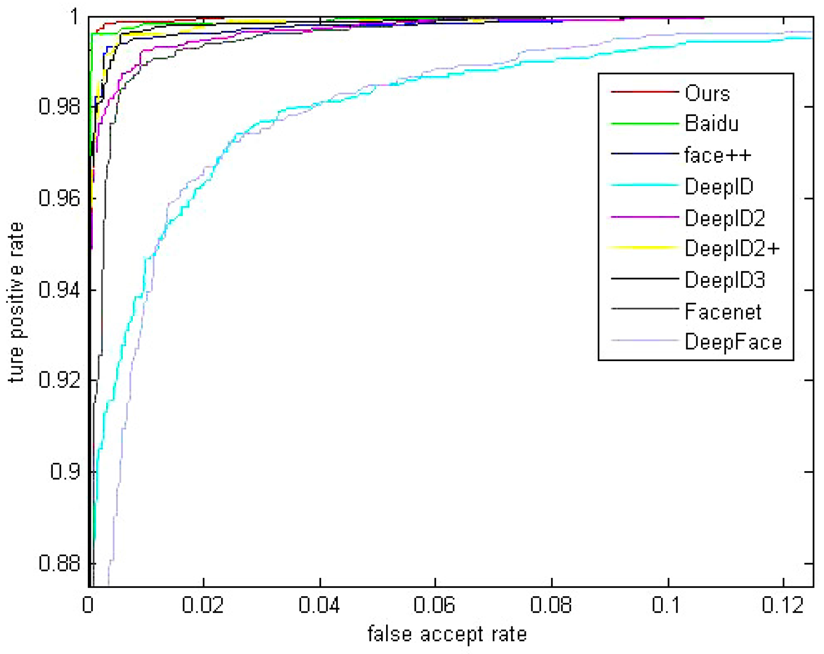
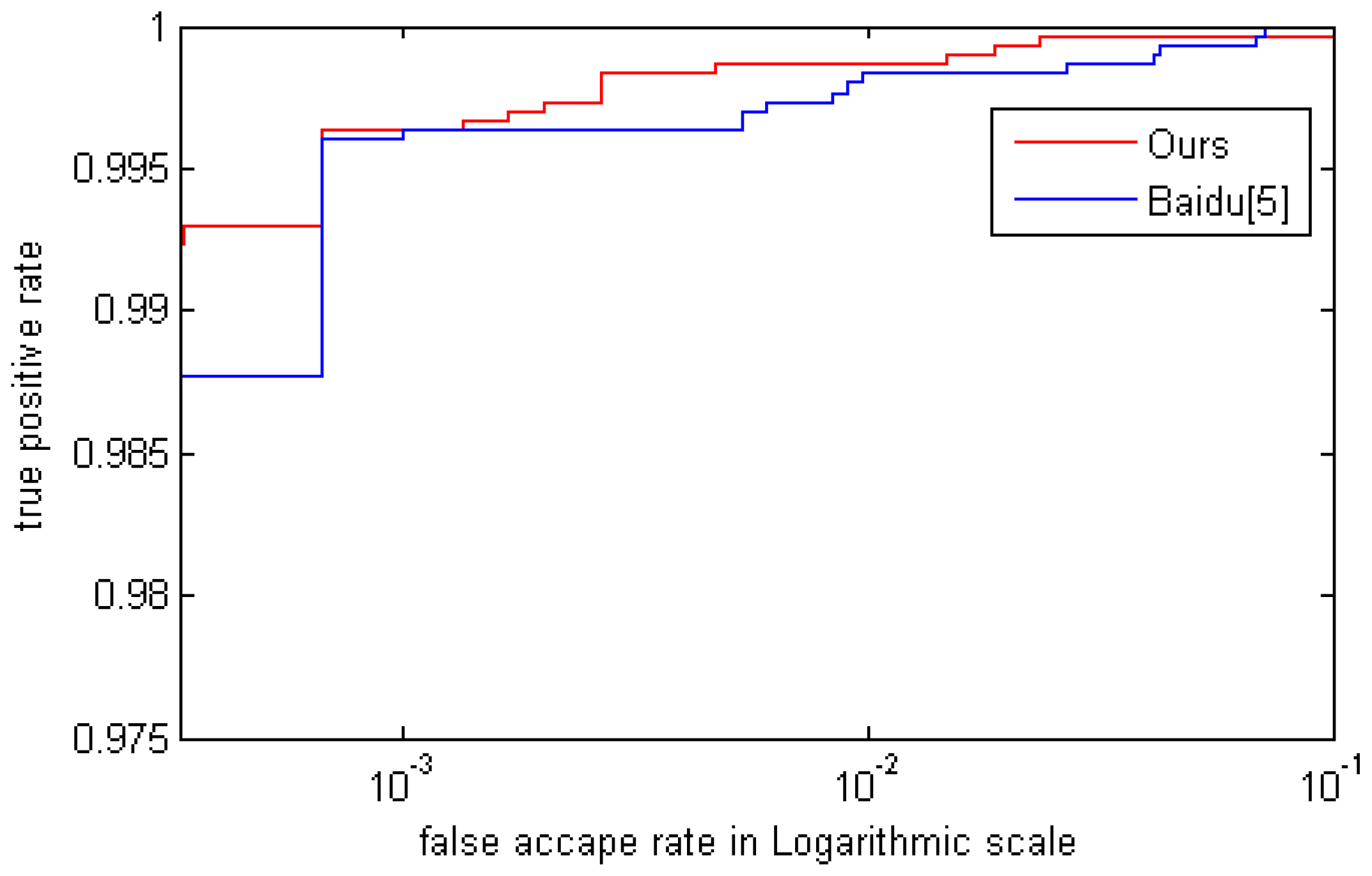
5.4. Comparision with Other Methods

To show the performance of our algorithm, we compare pairwise accuracy on the LFW dataset and the YTF dataset with the state-of-the-art deep methods.

In

Table 6. Accuracy of different methods on the LFW and YTF datasets.

Method	Accuracy on LFW	Identities	Face Number	Accuracy on YTF
Baidu [5]	99.77%	18 k	1.2 M	NA
Ours	99.71%	15 k	0.4 M	94.6%
Centerloss [12]	99.28%	17 k	0.7 M	94.9%
FaceNet [4]	99.63%	NA	260 M	95.1%
DeepID3 [25]	99.53%	16 k	NA	NA
Face++ [26]	99.50%	16 k	NA	NA
DeepID2+ [27]	99.47%	NA	NA	93.2%
DeepID2 [3]	99.15%	10 k	NA	NA
DeepFR [28]	98.95%	2.6 k	2.6 M	97.3%
DeepID [4]	97.45%	10 k	NA	NA
DeepFace [29]	97.35%	NA	NA	91.4%

, we show the results of comparisons and the scales of the database used for training in different methods. As a result, our method achieves 99.71% test accuracy, and it outperforms most deep face verification algorithms. The method in [5] is only 0.06% higher than ours, but the number of faces they used for training was 12 times the amount of data that we have. Therefore, our face verification method has a high product with a small cost.

Figure 10 compares receiver operating characteristic(ROC) curves of different methods, and the curve of our algorithm is much smoother than others. In the experiment, there are 17 wrong pairs in which three of them are wrongly labeled. Thus, our final pairwise accuracy is 99.75%. For safety, on some occasions such as financing institutions, a large true positive rate when the false acceptance rate is small is important. Though Baidu [5] got a better accuracy than us, according to Figure 11 and

Table 7. True Positive Rate (TPR) with different False Acceptance Rate (FAR).

Method	FAR = 0.03%	FAR = 0.1%	FAR = 1%
Baidu [2]	98.77%	99.63%	99.83%
Ours	99.3%	99.65%	99.87%

, we can see that when the false acceptance rate is small, our method will get a better true positive rate.

6. Conclusions

In this paper, we propose a face verification method based on multi-task and multi-scale features fusion with Joint Bayesian classifier. In addition, our algorithm has achieved high performance (99.75%) on the LFW dataset. Furthermore, we only use one region and one resolution in our face representation process. In addition, the training database that we used is small. Thus, our method is more practical in a real-life scenario.

References

1. Ren, S.; He, K.; Girshick, R.; Sun, J. Faster R-CNN: Towards real-time object detection with region proposal networks. arXiv, 2015; arXiv:1506.01497. [Google Scholar] [PubMed]
2. Long, J.; Shelhamer, E.; Darrell, T. Fully convolutional networks for semantic segmentation. In Proceedings of the IEEE Conference on Computer Vision and Pattern Recognition, Boston, MA, USA, 7–12 June 2015; pp. 3431–3440. [Google Scholar]
3. Krizhevsky, A.; Sutskever, I.; Hinton, G.E. Imagenet classification with deep convolutional neural networks. In Proceedings of the Twenty-Sixth Annual Conference on Neural Information Processing Systems (NIPS), Stateline, NV, USA, 3–8 December 2012; pp. 1097–1105. [Google Scholar]
4. Schroff, F.; Kalenichenko, D.; Philbin, J. Facenet: A unified embedding for face recognition and clustering. In Proceedings of the 2015 IEEE Conference on Computer Vision and Pattern Recognition (CVPR), Boston, MA, USA, 7–12 June 2015; pp. 815–823. [Google Scholar]
5. Liu, J.; Deng, Y.; Bai, T.; Wei, Z.P.; Huang, H. Targeting ultimate accuracy: Face recognition via deep embedding. arXiv, 2015; arXiv:1506.07310. [Google Scholar]
6. Sun, Y.; Wang, X.; Tang, X. Deep learning face representation by joint identification-verification. arXiv, 2014; arXiv:1406.4773. [Google Scholar]
7. Sun, Y.; Wang, X.; Tang, X. Deep learning face representation from predicting 10,000 classes. In Proceedings of the 2014 IEEE Conference on Computer Vision and Pattern Recognition, Columbus, OH, USA, 23–28 June 2014; pp. 1891–1898. [Google Scholar]
8. Simonyan, K.; Zisserman, A. Very deep convolutional networks for large-scale image recognition. arXiv, 2014; arXiv:1409.1556. [Google Scholar]
9. Szegedy, C.; Liu, W.; Jia, Y.; Sermanet, P.; Reed, S.; Anguelov, D.; Erhan, D.; Vanhoucke, V.; Rabinovich, A. Going deeper with convolutions. In Proceedings of the 2015 IEEE Conference on Computer Vision and Pattern Recognition (CVPR), Boston, MA, USA, 7–12 June 2015; pp. 1–9. [Google Scholar]
10. He, K.; Zhang, X.; Ren, S.; Sun, J. Deep residual learning for image recognition. In Proceedings of the 2016 IEEE Conference on Computer Vision and Pattern Recognition (CVPR), Las Vegas, NV, USA, 27–30 June 2016; pp. 770–778. [Google Scholar]
11. Chopra, S.; Hadsell, R.; Lee, C.Y. Learning a similarity metric discriminatively, with application to face verification. In Proceedings of the 2005 IEEE Computer Society Conference on Computer Vision and Pattern Recognition (CVPR’05), San Diego, CA, USA, 20–25 June 2005; pp. 539–546. [Google Scholar]
12. Wen, Y.; Zhang, K.; Li, Z.; Qiao, Y. A Discriminative Feature Learning Approach for Deep Face Recognition. In Proceedings of the European Conference on Computer Vision, Amsterdam, The Netherlands, 11–14 October 2016; pp. 11–26. [Google Scholar]
13. Yi, D.; Lei, Z.; Liao, S.; Li, S.Z. Learning face representation from scratch. arXiv, 2014; arXiv:1411.7923. [Google Scholar]
14. Lee, C.Y.; Xie, S.; Gallagher, P.; Zhang, Z.; Tu, Z. Deeply-Supervised Nets. arXiv, 2014; arXiv:1409.5185. [Google Scholar]
15. Song, H.O.; Xiang, Y.; Jegelka, S.; Savarese, S. Deep metric learning via lifted structured feature embedding. arXiv, 2015; arXiv:1511.06452. [Google Scholar]
16. Ioffe, S.; Szegedy, C. Batch normalization:Accelerating deep network training by reducing internal covariate shift. arXiv, 2015; arXiv:1502.03167. [Google Scholar]
17. Nair, V.; Hinton, G.E. Rectified linear units improve restricted boltzmann machines. In Proceedings of the 27th International Conference on Machine Learning, Haifa, Israel, 21–24 June 2010; pp. 807–814. [Google Scholar]
18. Szegedy, C.; Ioffe, S.; Vanhoucke, V.; Alemi, A. Inception-v4, inception-resnet and the impact of residual connections on learning. arXiv, 2016; arXiv:1602.07261. [Google Scholar]
19. Yang, S.; Luo, P.; Loy, C.C.; Tang, X. From facial parts responses to face detection: A deep learning approach. In Proceedings of the 2015 IEEE International Conference on Computer Vision (ICCV), Santiago, Chile, 7–13 December 2015; pp. 3676–3684. [Google Scholar]
20. Ye, M.; Wang, X.; Yang, R.; Ren, L.; Pollefeys, M. Accurate 3d pose estimation from a single depth image. In Proceedings of the 2011 International Conference on Computer Vision, Barcelona, Spain, 6–13 November 2011; pp. 731–738. [Google Scholar]
21. Chen, D.; Cao, X.; Wang, L.; Wen, F.; Sun, J. Bayesian face revisited: A joint formulation. In Proceedings of the 12th European Conference on Computer Vision, Florence, Italy, 7–13 October 2012; pp. 566–579. [Google Scholar]
22. Jia, Y.; Shelhamer, E.; Donahue, J.; Karayev, S.; Long, J.; Girshick, R.; Guadarrama, S.; Darrell, T. Caffe: Convolutional architecture for fast feature embedding. arXiv, 2014; arXiv:1408.5093. [Google Scholar]
23. Huang, G.B.; Ramesh, M.; Berg, T.; Learned-Miller, E. Labeled Faces in the Wild: A Database for Studying Face Recognition in Unconstrained Environments; Technical Report; University of Massachusetts: Amherst, MA, USA, 2007; pp. 7–49. [Google Scholar]
24. Wolf, L.; Hassner, T.; Maoz, I. Face recognition in unconstrained videos with matched background similarity. In Proceedings of the 2011 IEEE Conference on Computer Vision and Pattern Recognition (CVPR), Colorado Springs, CO, USA, 20–25 June 2011; pp. 529–534. [Google Scholar]
25. Sun, Y.; Liang, D.; Wang, X.; Tang, X. Deepid3: Face recognition with very deep neural networks. arXiv, 2015; arXiv:1502.00873. [Google Scholar]
26. Zhou, E.; Cao, Z.; Yin, Q. Naive-deep face recognition: Touching the limit of LFW benchmark or not? arXiv, 2015; arXiv:1501.04690. [Google Scholar]
27. Sun, Y.; Wang, X.; Tang, X. Deeply learned face representations are sparse, selective, and robust. In Proceedings of the 2015 IEEE Conference on Computer Vision and Pattern Recognition (CVPR), Boston, MA, USA, 7–12 June 2015; pp. 2892–2900. [Google Scholar]
28. Parkhi, O.M.; Vedaldi, A.; Zisserman, A. Deep Face Recognition. In Proceedings of the British Machine Vision Conference (BMVC), Swansea, UK, 7–10 September 2015; pp. 1–12. [Google Scholar]
29. Taigman, Y.; Yang, M.; Ranzato, M.A.; Wolf, L. Deepface: Closing the gap to human-level performance in face verification. In Proceedings of the 2014 IEEE Conference on Computer Vision and Pattern Recognition, Columbus, OH, USA, 23–28 June 2014; pp. 1701–1708. [Google Scholar]
Figure 1. The overall framework of face verification.
Entropy 19 00228 g001
Figure 2. An example of random selection. Rounds present image pairs, which are selected for computing semi-verification loss. Diamonds are not selected. They belong to the same identity and there is no connection between circles and diamonds.
Entropy 19 00228 g002
Figure 3. The method of instituting image pairs. f i ( i = 1 , 2 , · · · , n ) present the face image of a certain person.
Entropy 19 00228 g003
Figure 4. Inception used in CNN1.
Entropy 19 00228 g004
Figure 5. The overall frameworks of CNNs.
Entropy 19 00228 g005
Figure 6. Res-Inception used in CNN2.
Entropy 19 00228 g006
Figure 7. Face normalization by eye centers and distance.
Entropy 19 00228 g007
Figure 8. The flow chart of face normalization.
Entropy 19 00228 g008
Figure 9. The loss of different values of λ .
Entropy 19 00228 g009
Figure 10. ROC curves of different methods.
Entropy 19 00228 g010
Figure 11. ROC curves of Baidu [5] and ours.
Entropy 19 00228 g011