Article

Specific and Complete Local Integration of Patterns in Bayesian Networks

1
Araya Incorporation, 2F Mori 15 Building, 2-8-10 Toranomon, Minato-ku, Tokyo 105-0001, Japan
2
School of Computer Science, University of Hertfordshire, Hatfield AL10 9AB, UK
3
Department of General Systems Studies, University of Tokyo, 3-8-1 Komaba, Meguro-ku, Tokyo 153-8902, Japan
*
Author to whom correspondence should be addressed.
Entropy 2017, 19(5), 230; https://doi.org/10.3390/e19050230
Submission received: 19 March 2017 / Revised: 11 May 2017 / Accepted: 12 May 2017 / Published: 18 May 2017
(This article belongs to the Special Issue Complexity, Criticality and Computation (C³))

Abstract

:
We present a first formal analysis of specific and complete local integration. Complete local integration was previously proposed as a criterion for detecting entities or wholes in distributed dynamical systems. Such entities in turn were conceived to form the basis of a theory of emergence of agents within dynamical systems. Here, we give a more thorough account of the underlying formal measures. The main contribution is the disintegration theorem which reveals a special role of completely locally integrated patterns (what we call ι-entities) within the trajectories they occur in. Apart from proving this theorem we introduce the disintegration hierarchy and its refinement-free version as a way to structure the patterns in a trajectory. Furthermore, we construct the least upper bound and provide a candidate for the greatest lower bound of specific local integration. Finally, we calculate the ι -entities in small example systems as a first sanity check and find that ι -entities largely fulfil simple expectations.

1. Introduction

This paper investigates a formal measure and a corresponding criterion we developed in order to capture the notion of wholes or entities within Bayesian networks in general and multivariate Markov chains in particular. The main focus of this paper is to establish some formal properties of this criterion.
The main intuition behind wholes or entities is that combinations of some events/phenomena in space(-time) can be considered as more of a single or coherent “thing” than combinations of other events in space(-time). For example, the two halves of a soap bubble (The authors thank Eric Smith for pointing out the example of a soap bubble.) together seem to form more of a single thing than one half of a floating soap bubble together with a piece of rock on the ground. Similarly, the soap bubble at time t 1 and the “same” soap bubble at t 2 seem more like temporal parts of the same thing than the soap bubble at t 1 and the piece of rock at t 2 . We are trying to formally define and quantify what it is that makes some spatially and temporally extended combinations of parts entities but not others.
We envisage spatiotemporal entities as a way to establish not only the problem of spatial identity but also that of temporal identity (also called identity over time [1]). In other words, in addition to determining which events in “space” (e.g., which values of different degrees of freedom) belong to the same structure spatiotemporal entities should allow the identification of the structure at a time t 2 that is the future (or past if t 2 < t 1 ) of a structure at time t 1 . Given a notion of identity over time, it becomes possible to capture which things persist and in what way they persist. Without a notion of identity over time, it seems persistence is not defined. The problem is how to decide whether something persisted from t 1 to t 2 if we cannot tell what at t 2 would count as the future of the original thing.
In everyday experience problems concerning identity over time are not of great concern. Humans routinely and unconsciously connect perceived events to spatially and temporally extended entities. Nonetheless, the problem has been known since ancient times, in particular with respect to artefacts that exchange their parts over time. A famous example is the Ship of Theseus which has all of its planks exchanged over time. This leads to the question whether it is still the same ship. From the point of view of physics and chemistry living organisms also exchange their parts (e.g., the constituting atoms or molecules) over time. In the long term we hope our theory can help to understand identity over time for these cases. For the moment, we are particularly interested in identity over time in formal settings like cellular automata, multivariate Markov chains, and more generally dynamical Bayesian networks. In these cases a formal notion of spatiotemporal entities (i.e., one defining spatial and temporal identity) would allow us to investigate persistence of entities/individuals formally. The persistence (and disappearance) of individuals are in turn fundamental to Darwinian evolution [2,3]. This suggests that spatiotemporal entities may be important for the understanding of the emergence of Darwinian evolution in dynamical systems.
Another area in which a formal solution to the problem of identity over time, and thereby entities (In the following, if not stated otherwise, we always mean spatiotemporal entities when we refer to entities.), might become important is a theory of intelligent agents that are space-time embedded as described by Orseau and Ring [4]. Agents are examples of entities fulfilling further properties e.g., exhibition of actions, and goal-directedness (cf. e.g., [5]). Using the formalism of reinforcement learning Legg and Hutter [6] proposes a definition of intelligence. Orseau and Ring [4] argue that this definition is insufficient. They dismiss the usual assumption that the environment of the reinforcement agent cannot overwrite the agent’s memory (which in this case is seen as the memory/tape of a Turing machine). They conclude that in the most realistic case there only ever is one memory that the agent’s (and the environment’s) data is embedded in. They note that the difference between agent and environment then disappears. Furthermore, that the policy of the agent cannot be freely chosen anymore, only the initial condition. In order to measure intelligence according to Legg and Hutter [6] we must be able to define reward functions. This seems difficult without the capability to distinguish the agent according to some criterion. Towards the end of their publication Orseau and Ring [4] propose to define a “heart” pattern and use the duration of its existence as a reward. This seems a too specific approach to us since it basically defines identity over time (of the heart pattern) as invariance. In more general settings a pattern that maintains a more general criterion of identity over time would be desirable. Ideally, this criterion would also not need a specifically designed heart pattern. Another advantage would be that reward functions different from lifetime could be used if the agent were identifiable. An entity criterion in the sense of this paper would be a step in this direction.

1.1. Illustration

In order to introduce the contributions of this paper we illustrate the setting of our work further.
This illustration should only be taken as a motivation for what follows and not be confused with a result. The reason we don’t use a concrete example is simply that we lack the necessary computational means (which are considerable as we will discuss in Section 5).
Let us assume we are given the entire time-evolution (what we will call a trajectory) of some known multivariate dynamical system or stochastic process. For example, a trajectory of a one-dimensional elementary cellular automaton showing a glider collision like Figure 1a (This is produced by the rule 62 elementary cellular automaton with time increasing from left to right. However, this does not matter here. For more about this system see e.g., Boccara et al. [7]).
We take the point of view here argued for in previous work [8] that entities are phenomena that occur within trajectories and that they can be represented by (spatiotemporal) patterns. Patterns in this sense fix a part of the variables in a trajectory to definite values and leave the rest undetermined. In Figure 1b–d we show such patterns that occur in Figure 1a with the undetermined variables coloured grey and the determined ones taking on those of the trajectory. Visually speaking, a pattern is a snippet from a trajectory that it occurs in.
From Figure 1a we would probably expect that what we are seeing are two gliders colliding and forming a third. However, it may also be that one of the gliders absorbs the other, maintains some form of identity, and only changes its appearance (e.g., it “grows”). This highlights the problem of identity over time. While the spatial identity of such patterns has been treated multiple times in the literature their identity of over time is rarely dealt with.
Our approach evaluates the “integration” of spatiotemporally extended patterns at once. According to our proposed entity-criterion a pattern is an ι -entity if, due to the dynamics of the system, every part of this pattern (which is again a pattern) makes all other parts more probable. Identity over time is then included since future parts have to make past parts more probable and vice versa. In principle this would allow us to detect if one of the gliders absorbs another one without loosing its identity. For example, this could result in an entity as in Figure 1e.
In order to detect entities the straightforward approach is to evaluate the entity-criterion for every spatiotemporal pattern in a given trajectory. Evaluating our entity-criterion of positive complete local integration (CLI) for a given pattern corresponds to splitting the pattern into parts in every possible way and calculating whether all the resulting parts make each other more probable. This means evaluating the specific local integration (SLI) with respect to all partitions of the set of variables occupied by the pattern.

1.2. Contributions

This paper contains four contributions.
We first give a more formal definition of patterns. Since each pattern uniquely specifies a set of trajectories (those trajectories that the pattern occurs in) one might be tempted to reduce the analysis to that of sets of trajectories. We show that this is not possible since not all sets of trajectories have a pattern that specifies them.
Second, we try to get a general intuition for the patterns whose parts make all other parts more probable. For this we show how to construct patterns that, for given probability of the whole pattern, achieve the least upper bound of specific local integration (SLI). These turn out to be patterns for which each part only occurs if and only if the whole pattern occurs. We also construct a pattern that, again for given probability of the whole pattern, has negative SLI. These pattern (which may achieve the greatest lower bound of SLI) occur if either the whole pattern occurs or the pattern occurs up to exactly one part of it, which does not occur.
Third, we prove the disintegration theorem. This is the main contribution. We saw that patterns are snippets of trajectories. We can also look at the whole trajectory as a single pattern. Like all patterns the trajectory can be split up into parts, i.e., partitioned, resulting in a set of patterns. Among the partitions we find examples such as those in Figure 1g,h. These are very particular partitions picking out the gliders among all possible parts. This suggests that finding such special partitions provides a (possibly different) notion of entities.
One intuition we might have is that entities are the most “independent” parts of a trajectory. In other words we could look for the partition whose parts make the other parts less probable. The disintegration theorem then shows that this approach again leads to the ι -entities. This shows that ι -entities do not only have an intuitive motivation but also play a particular role in the structure of probabilities of entire trajectories.
It is not directly the parts of the partitions that minimise SLI for a trajectory which are ι -entities. To get ι -entities we first classify all partitions of the trajectory according to their SLI value. Then within each such class we choose the partitions for which no refining partition (A refining partition is one that further partitions any of the parts of the original partition.) achieves an even lower level of SLI.
So according to the disintegration theorem a ι -entity is not only a pattern that is integrated with respect to every possible partition of the pattern but also a pattern that occurs in partitions that minimise (in a certain sense) the integration of trajectories.
A side effect of the disintegration theorem is that we naturally get a kind of hierarchy of ι -entities called the disintegration hierarchy. For each trajectory and its different levels of SLI we find different decompositions of the trajectory into ι -entities.
Fourth, we calculate the ι -entities and disintegration hierarchy for two simple example systems. Our example systems show that in general the partitions at a particular disintegration level are not unique. This means that there are overlapping ι -entities at those levels. Furthermore, the same ι -entity can occur on multiple levels of the disintegration.
We do not thoroughly discuss the disintegration hierarchies in this paper and postpone this to future publications. Here we only note that many entities in the real world occur within hierarchies as well. For example, animals are entities that are composed of cells which are themselves entities.

1.3. Related Work

We now give a quick overview of related work. More in depth discussions will be provided after we formally introduce our definitions.
To our knowledge the measure of CLI has been proposed for the first time by us in [8]. However, this publication contained none of the formal or numerical results in the present paper. From a formal perspective the measures of SLI and CLI are a combination of existing concepts. SLI localises multi-information [9,10] in the way proposed by Lizier [11] for other information theoretic measures. In order to get the CLI we apply the weakest-link approach proposed by Tononi and Sporns [12], Balduzzi and Tononi [13] to SLI.
Conceptually, our work is most closely related to Beer [14]. The notion of spatiotemporal patterns used there to capture blocks, blinkers, and gliders is equivalent to the patterns we define more formally here. This work also contains an informal entity-criterion that directly deals with identity over time (not only space). It differs significantly from our proposal as it depends on the re-occurrence of certain transitions at later times in a pattern whereas our criterion only depends on the probabilities of parts of the patterns without the need for any re-occurrences.
The organisations of chemical organisation theory [15] may also be interpreted as entity-criteria. In Fontana and Buss [15] these are defined in the following way:
The observer will conclude that the system is an organisation to the extent that there is a compressed description of its objects and of their relations.
The direct intuition is different from ours and it is not clear to us in how far our entity-criterion is equivalent to this. This will be further investigated in the future.
It is worth noting that viewing entities/objects/individuals as patterns occurring within a trajectory is in contrast to an approach that models them as sets of random variables/stochastic processes (e.g., a set of cells in a CA in contrast to a set of specific values of a set of cells). An example of the latter approach are the information theoretic individuals of Krakauer et al. [16]. These individuals are identified using an information theoretic notion of autonomy due to Bertschinger et al. [17]. The latter notion of autonomy is also somewhat related to the idea of integration here. Autonomy contains a term that measures the degree to which a random variable representing an individual at timestep t determines the random variable representing it at t + 1 . Similarly, CLI requires that every part of an entity pattern makes every other part more probable, in the extreme case this means that every part determines that every other part of the pattern also occurs. However, formally autonomy evaluates random variables and not patterns directly.
At the most basic level the intuition behind entities is that some spatiotemporal patterns are more special than others. Defining (and usually finding) more important spatiotemporal patterns or structures (also called coherent structures) has a long history in the theory of cellular automata and distributed dynamical systems. As Shalizi et al. [18] have argued most of the earlier definitions and methods [19,20,21,22] require previous knowledge about the patterns being looked for. They are therefore not suitable for a general definition of entities. More recent definitions based on information theory [18,23,24] do not have this limitation anymore. The difference to our entity-criterion is that they do not treat identity over time. They are well suited to identify gliders at each time-step for example, but if two gliders collide and give rise to a third glider as in Figure 1a these methods (by design) say nothing about the identity of the third glider. i.e., they cannot make a difference between a glider absorbing another one and two gliders producing a new one. While we have not been able to show that our approach actually makes such distinctions for gliders, it could do so in principle.
We note here that the approach of identifying individuals by Friston [25] using Markov blankets has the same shortcoming as the spatiotemporal filters. For each individual time-step it returns a partition of all degrees of freedom into internal, sensory, active, and external degrees. However, it does not provide a way to resolve ambiguities in the case of multiple such partitions colliding.
Among research related to integrated information theory (IIT) there are approaches (a first one by Balduzzi [26] and a more recently by Hoel et al. [27]) that can be used to determine specific spatiotemporal patterns in a trajectory. They can therefore be interpreted to define a notion of entities even if that is not their main goal. These approaches are aimed at establishing the optimal spatiotemporal coarse-graining to describe the dynamics of a system. For a given trajectory we can then identify the patterns that instantiate a macro-state/coarse-grain that is optimal according to their criterion.
In contrast to our approach the spatiotemporal grains are determined by their interactions with other grains. In our case the entities are determined first and foremost by their internal relations.
The consequence seems to be that a pattern can be an entity in one trajectory and not an entity in another even if it occurs in both. In our conception a pattern is an entity in all trajectories it occurs in.

2. Notation and Background

In this section we briefly introduce our notation for sets of random variables (Since every set of jointly distributed random variables can be seen as a Bayesian network and vice versa we use these terms interchangeably.) and their partition lattices.
In general, we use the convention that upper-case letters X , Y , Z are random variables, lower-case letters x , y , z are specific values/outcomes of random variables, and calligraphic letters X , Y , Z are state spaces that random variables take values in. Furthermore:
Definition 1.
Let { X i } i V be a set of random variables with totally ordered finite index set V and state spaces { X i } i V respectively. Then for A , B V define:
1. 
X A : = ( X i ) i A as the joint random variable composed of the random variables indexed by A, where A is ordered according to the total order of V,
2. 
X A : = i A X i as the state space of X A ,
3. 
x A : = ( x i ) i A X A as a value of X A ,
4. 
p A : X A [ 0 , 1 ] as the probability distribution (or more precisely probability mass function) of X A which is the joint probability distribution over the random variables indexed by A. If A = { i } i.e., a singleton set, we drop the parentheses and just write p A = p i ,
5. 
p A , B : X A × X B [ 0 , 1 ] as the probability distribution over X A × X B . Note that in general for arbitrary A , B V , x A X A , and y B X B this can be rewritten as a distribution over the intersection of A and B and the respective complements. The variables in the intersection have to coincide:
p A , B ( x A , y B ) : = p A \ B , A B , B \ A , A B ( x A \ B , x A B , y B \ A , y A B )
= δ x A B ( y A B ) p A \ B , A B , B \ A ( x A \ B , x A B , y B \ A ) .
Here δ is the Kronecker delta (see Appendix A). If A B = and C = A B we also write p C ( x A , y B ) to keep expressions shorter.
6. 
p B | A : X A × X B [ 0 , 1 ] with ( x A , x B ) p B | A ( x B | x A ) as the conditional probability distribution over X B given X A :
p B | A ( y B | x A ) : = p A , B ( x A , y B ) p A ( x A ) .
We also just write p B ( x B | x A ) if it is clear from context what variables we are conditioning on.
If we are given p V we can obtain every p A through marginalisation. In the notation of Definition 1 this is formally written:
p A ( x A ) = x ¯ V \ A X V \ A p A , V \ A ( x A , x ¯ V \ A )
= x ¯ V \ A X V \ A p V ( x A , x ¯ V \ A ) .
Next we define the partition lattice of a set of random variables. Partition lattices occur as a structure of the set of possible ways to split an object/pattern into parts. Subsets of the partition lattices play an important role in the disintegration theorem.
Definition 2 (Partition lattice of a set of random variables).
Let { X i } i V be a set of random variables.
1. 
Then its partition lattice L ( V ) is the set of partitions of V partially ordered by refinement (see also Appendix B).
2. 
For two partitions π , ρ L ( V ) we write π ρ if π refines ρ and π : ρ if π covers ρ. The latter means that π ρ , π ρ , and there is no ξ L ( V ) with π ξ ρ such that π ξ ρ .
3. 
We write 0 for the zero element of a partially ordered set (including lattices) and 1 for the unit element.
4. 
Given a partition π L ( V ) and a subset A V we define the restricted partition π | A of π to A via:
π | A : = { b A : b π } .
For some examples of partition lattices see Appendix B and for more background see e.g., Grätzer [28]. For our purpose it is important to note that the partitions of sets of random variables or Bayesian networks we are investigating are partitions of the index set V of these and not partitions of their state spaces X V .

3. Patterns, Entities, Specific, and Complete Local Integration

This section contains the formal part of this contribution.
First we introduce patterns. Patterns are the main structures of interest in this publication. Entities are seen as special kinds of patterns. The measures of specific local integration and complete local integration, which we use in our criterion for ι -entities, quantify notions of “oneness” of patterns. We give a brief motivation and show that while each pattern defines a set of “trajectories” of a set of random variables not every such set is defined by a pattern. This justifies studying patterns for their own sake.
Then we motivate briefly the use of specific and complete local integration (SLI and CLI) for an entity criterion on patterns. We then turn to more formal aspects of SLI and CLI. We first prove an upper bound for SLI and construct a candidate for a lower bound. We then go on to define the disintegration hierarchy and its refinement-free version. These structures are used to prove the main result, the disintegration theorem. This relates the SLI of whole trajectories of a Bayesian network to the CLI of parts of these trajectories and vice versa.

3.1. Patterns

This section introduces the notion of patterns. These form the basic candidate structures for entities.
The structures we are trying to capture by entities should be analogous to spatially and temporally extended objects we encounter in everyday life (e.g., soap bubbles, living organisms). These objects seem to occur in the single history of the universe that also contains us. The purpose of patterns is then to capture arbitrary structures that occur within single trajectories or histories of a multivariate discrete dynamical system (see Figure 2 for an example of a Bayesian network of such a system, any cellular automaton is also such a system).
We emphasise the single trajectory since many structures of interest (e.g., gliders) occur in some trajectories in some “places”, in other trajectories in other “places” (compare e.g., Figure 1a and Figure 3a), and in some trajectories not at all. We explicitly want to be able to capture such trajectory dependent structures and therefore choose patterns. Examples of formal structures for which it makes no sense to say that they occur within a trajectory are for example the random variables in a Bayesian network and, as we will see, general sets of trajectories of the Bayesian network.
Unlike entities, which we conceive of as special patterns that fulfil further criteria, patterns are formed by any combination of events at arbitrary times and positions. As an example, we might think of cellular automaton again. The time evolutions over multiple steps of the cells attributed to a glider see [14] for a principled way to attribute cells to theseas in Figure 1b,e should be patterns but also arbitrary choices of events in a trajectory as in Figure 3b.
In the more general context of (finite) Bayesian networks there may be no interpretation of time or space. Nonetheless, we can define that a trajectory in this case fixes every random variable to a particular value. We then define patterns formally in the following way.
Definition 3 (Patterns and trajectories).
Let { X i } i V be set of random variables with index set V and state spaces { X i } i V respectively.
1. 
A pattern at A V is an assignment
X A = x A
where x A X A . If there is no danger of confusion we also just write x A for the pattern X A = x A at A.
2. 
The elements x V of the joint state space X V are isomorphic to the patterns X V = x V at V which fix the complete set { X i } i V of random variables. Since they will be used repeatedly we refer to them as the trajectories of { X i } i V .
3. 
A pattern x A is said to occur in trajectory x ¯ V X V if x ¯ A = x A .
4. 
Each pattern x A uniquely defines (or captures) a set of trajectories T ( x A ) via
T ( x A ) = { x ¯ V X V : x ¯ A = x A } ,
i.e., the set of trajectories that x A occurs in.
5. 
It is convenient to allow the empty pattern x for which we define T ( x ) = X V .
Remarks:
  • Note that for every x A X A we can form a pattern X A = x A so the set of all patterns is A V X A .
  • Our notion of patterns is similar to “patterns” as defined in [29] and to “cylinders” as defined in [30]. More precisely, these other definitions concern (probabilistic) cellular automata where all random variables have identical state spaces X i = X j for all i , j V . They also restrict the extent of the patterns or cylinders to a single time-step. Under these conditions our patterns are isomorphic to these other definitions. However, we drop both the identical state space assumption and the restriction to single time-steps.
    Our definition is inspired by the usage of the term “spatiotemporal pattern” in [14,31,32]. There is no formal definition of this notion given in these publications but we believe that our definition is a straightforward formalisation. Note that these publications only treat the Game of Life cellular automaton. The assumption of identical state space is therefore implicitly made. At the same time the restriction to single time-steps is explicitly dropped.
Since every pattern defines a subset of X V , one could think that every subset of X V is also a pattern. In that case studying patterns in a set of random variables { X i } i V would be the same as studying subsets of its set of trajectories X V . However, the set of subsets of X V defined by patterns and the set of all subsets 2 X V (i.e., the power set) of X V of a set of random variables { X i } i V are not identical. Formally:
B V { T ( x B ) X V : x B X B } 2 X V .
While patterns define subsets of X V , not every subset of X V is captured by a pattern. The difference of the two sets is characterised in Theorem 1 below. We first present a simple example of a subset D 2 X V that cannot be captured by a pattern.
Let V = { 1 , 2 } and { X i } i V = { X 1 , X 2 } the set of random variables. Let X 1 = X 2 = { 0 , 1 } . Then X V = { ( 0 , 0 ) , ( 0 , 1 ) , ( 1 , 0 ) , ( 1 , 1 ) } . Now let A = V = { 1 , 2 } , choose pattern x A = ( 0 , 0 ) and pattern x ¯ A = ( 1 , 1 ) . Then let
D : = { x A x ¯ A } = { ( 0 , 0 ) , ( 1 , 1 ) } .
In this case we can easily list the set of all patterns C V X C :
Entropy 19 00230 i001
and verify that D is not among them. Before we formally characterise the difference, we define some extra terminology.
Definition 4.
Let { X i } i V be set of random variables with index set V and state spaces { X i } i V respectively. For a subset D X V the set D A of all patterns at A that occur in one of the trajectories in D is defined as
D A : = { x A X A : x ¯ V D , x ¯ A = x A } .
So in the previous example D { 1 } = { 0 , 1 } , D { 2 } = { 0 , 1 } , D { 1 , 2 } = { ( 0 , 0 ) , ( 1 , 1 ) } . In then get the following theorem which establishes the difference between the subsets of X V captured by patterns and general subsets.
Theorem 1.
Given a set of random variables { X i } i V , a subset D X V cannot be represented by a pattern of { X i } i V if and only if there exists A V with D A X A (proper subset) and | D A | > 1 , i.e., if neither all patterns at A are possible nor a unique pattern at A is specified by D .
Proof. 
See Appendix D. ☐
We saw that in the previous example the subset D cannot be captured by a pattern. For A = { 1 } we have D { 1 } = { 0 , 1 } = X { 1 } and for A = { 2 } we have D { 2 } = { 0 , 1 } = X { 2 } so these do not fulfil the conditions of Theorem 1. However, for A = { 1 , 2 } we have D { 1 , 2 } = { ( 0 , 0 ) , ( 1 , 1 ) } X { 1 , 2 } and | D { 1 , 2 } | > 1 so the conditions of Theorem 1 are fulfilled and as expected D cannot be captured by a pattern.
The proof of the following corollary shows how to construct a subset that cannot be represented by a pattern for all sets of random variables { X i } i V with | X V | > 2 .
Corollary 1.
Given a set of random variables { X i } i V , if | X V | > 2 then
B V { T ( x B ) X V : x B X B } 2 X V
(proper subset).
Proof. 
Choose D = { x V , y V } 2 X V with y V { x ¯ V X V : i V , x ¯ i x i } . Then for all A V we have | D A | = 2 and D A X A . So D cannot be represented by a pattern according to Theorem 1 and so D B V { T ( x B ) X V : x B X B } . ☐
This means that in every set of random variables that not only consists of a single binary random variable there are subsets of X V that cannot be captured by a pattern. We can interpret this result in the following way. Patterns were constructed to be structures that occur within trajectories. It then turned out that each pattern also defines a subset of all trajectories of a system. So for sets of trajectories captured by patterns it could make sense to say they “occur” within one trajectory. However, there are sets of trajectories that are not captured by patterns. For these sets of trajectories it would then not be well-defined to say that they occur within a trajectory. This is the reason we choose to investigate patterns specifically and not sets of trajectories.

3.2. Motivation of Complete Local Integration as an Entity Criterion

We proposed to use patterns as the candidate structures for entities since patterns comprise arbitrary structures that occur within single trajectories of multivariate systems. Here we heuristically motivate our choice of using positive complete local integration as a criterion to select entities among patterns. In general such a criterion would give us, for any Bayesian network { X i } i V a subset E ( { X i } i V ) A V X A of the patterns.
So what is an entity? We can rephrase the problem of finding an entity criterion by saying an entity is composed of parts that share the same identity. So if we can define when parts share the same identity we also define entities by finding all parts that share identity with some given part. For the moment, let us decompose (as is often done [33]) the problem of identity into two parts:
  • spatial identity and
  • temporal identity.
Our solution will make no distinction between these two aspects in the end. We note here that conceiving of entities (or objects) as composite of spatial and temporal parts as we do in this paper is referred to as four-dimensionalism or perdurantism in philosophical discussions (see e.g., [34]). The opposing view holds that entities are spatial only and endure over time. This view is called endurantism. Here we will not go into the details of this discussion.
The main intuition behind complete local integration is that every part of an entity should make every other part more probable.
This seems to hold for example for the spatial identity of living organisms. Parts of living organisms rarely exist without the rest of the living organisms also existing. For example, it is rare that an arm exists without a corresponding rest of a human body existing compared to an arm and the rest of a human body existing. The body (without arm) seems to make the existence of the arm more probable and vice versa. Similar relations between parts seem to hold for all living organisms but also for some non-living structures. The best example of a non-living structure we know of for which this is obvious are soap bubbles. Half soap bubbles (or thirds, quarters,...) only ever exist for split seconds whereas entire soap bubbles can persist for up to minutes. Any part of a soap bubble seems to make the existence of the rest more probable. Similarly, parts of hurricanes or tornadoes are rare. So what about spatial parts of structures that are not so entity-like? Does the existence of an arm make things more probable that are not parts of the corresponding body? For example, does the arm make the existence of some piece of rock more probable? Maybe to a small degree as without the existence of any rocks in the universe humans are probably impossible. However, this effect is much smaller than the increase of probability of the existence of the rest of the body due to the arm.
These arguments concerned the spatial identity problem. However, for temporal identity similar arguments hold. The existence of a living organism at one point in time makes it more probable that there is a living organism (in the vicinity) at a subsequent (and preceding) point in time. If we look at structures that are not entity-like with respect to the temporal dimension we find a different situation. An arm at some instance of time does not make the existence of a rock at a subsequent instance much more probable. It does make the existence of a human body at a subsequent instance much more probable. So the human body at the second instance seems to be more like a future part of the arm than the rock. Switching now to patterns in sets of random variables we can easily formalise such intuitions. We required that for an entity every part of the structure, which is now a pattern x O , makes every other part more probable. A part of a pattern is a pattern x b with b O . If we require that every part of a pattern makes every other part more probable then we can write that x O is an entity if:
min b O p O \ b ( x O \ b | x b ) p O \ b ( x O \ b ) > 1 .
This is equivalent to
min b O p O ( x O ) p O \ b ( x O \ b ) p b ( x b ) > 1 .
If we write L 2 ( O ) for the set of all bipartitions of O we can rewrite this further as
min π L 2 ( O ) p O ( x O ) b π p b ( x b ) > 1 .
We can interpret this form as requiring that for every possible partition π L 2 ( O ) into two parts x b 1 , x b 2 the probability of the whole pattern x O = ( x b 1 , x b 2 ) is bigger than its probability would be if the two parts were independent. To see this, note that if the two parts x b 1 , x b 2 were independent we would have
p O ( x O ) = : p b 1 , b 2 ( x b 1 , x b 2 ) = p b 1 ( x b 1 ) p b 2 ( x b 2 ) .
Which would give us
p O ( x O ) b π p b ( x b ) = 1
for this partition.
From this point of view the choice of bipartitions only seems arbitrary. For example, the existence a partition ξ into three parts such that
p O ( x O ) = c ξ p c ( x c )
seems to suggest that the pattern x O is not an entity but instead composite of three parts. We can therefore generalise Equation (16) to include all partitions L ( O ) (see Definition 2) of O except the unit partition 1 O . Then we would say that x O is an entity if
min π L ( O ) \ 1 O p O ( x O ) b π p b ( x b ) > 1 .
This measure already results in the same entities as the measure we propose.
However, in order to connect with information theory, log-likelihoods, and related literature we formally introduce the logarithm into this equation. We then arrive at the following entity-criterion
min π L ( O ) \ 1 O log p O ( x O ) b π p b ( x b ) > 0 .
where the left hand side is the complete local integration (CLI), the function minimised is the specific local integration (SLI), and the inequality provides the criterion for ι -entities. For reference, we define these notions formally. We begin with SLI which quantifies for a given partition π of a pattern in how far the probability of the whole pattern is bigger than its probability would be if the blocks of the partition would be independent.
Definition 5 (Specific local integration (SLI)).
Given a Bayesian network { X } i V and a pattern x O the specific local integration mi π ( x O ) of x O with respect to a partition π of O V is defined as
mi π ( x O ) : = log p O ( x O ) b π p b ( x b ) .
In this paper we use the convention that log 0 0 : = 0 .
Definition 6. ((Complete) local integration).
Given a Bayesian network { X i } i V and a pattern x O of this network the complete local integration ι ( x O ) of x O is the minimum SLI over the non-unit partitions π L ( O ) \ 1 O :
ι ( x O ) : = min π L ( O ) \ 1 O mi π ( x O ) .
We call a pattern x O completely locally integrated if ι ( x O ) > 0 .
Remarks:
  • The reason for excluding the unit partition 1 O of L ( O ) (where 1 O = { O } see Definition 2) is that with respect to it every pattern has mi 1 O ( x O ) = 0 .
  • Looking for a partition that minimises a measure of integration is known as the weakest link approach [35] to dealing with multiple partitions. We note here that this is not the only approach that is being discussed. Another approach is to look at weighted averages of all integrations. For a further discussion of this point in the case of the expected value of SLI see Ay [35] and references therein. For our interpretation taking the average seems less well suited since requiring a positive average will allow SLI to be negative with respect to some partitions.
Definition 7 (ι-entity).
Given a multivariate Markov chain { X i } i V a pattern x O is a ι-entity if
ι ( x O ) > 0 .
The entire set of ι -entities E ι ( { X i } i V ) is then defined as follows.
Definition 8 (ci-entity-set).
Given a multivariate Markov chain { X i } i V the ι-entity-set is the entity-set
E ι ( { X i } i V ) : = { x O A V X A : ι ( x O ) > 0 } .
Next, we look at some interpretations that the introduction of the logarithm allows.
  • A first consequence of introducing the logarithm is that we can now formulate the condition of Equation (24) analogously to an old phrase attributed to Aristotle that “the whole is more than the sum of its parts”. In our case this would need to be changed to “the log-probability of the (spatiotemporal) whole is greater than the sum of the log-probabilities of its (spatiotemporal) parts”. This can easily be seen by rewriting Equation (22) as:
    mi π ( x O ) = log p O ( x O ) b π log p b ( x b ) .
  • Another side effect of using the logarithm is that we can interpret Equation (24) in terms of the surprise value (also called information content) log p O ( x O ) [36] of the pattern x O and the surprise value of its parts with respect to any partition π . Rewriting Equation (22) using properties of the logarithm we get:
    mi π ( x O ) = b π ( log p b ( x b ) ) ( log p O ( x O ) ) .
    Interpreting Equation (24) from this perspective we can then say that a pattern is an entity if the sum of the surprise values of its parts is larger than the surprise value of the whole.
  • In coding theory, the Kraft-McMillan theorem [37] tells us that the optimal length (in a uniquely decodable binary code) of a codeword for an event x is l ( x ) = log p ( x ) if p ( x ) is the true probability of x. If the encoding is not based on the true probability of x but instead on a different probability q ( x ) then the difference between the optimal codeword length and the chosen codeword length is
    log q ( x ) ( log p ( x ) ) = log p ( x ) q ( x ) .
    Then we can interpret the specific local integration as a difference in codeword lengths. Say we want to encode what occurs at the nodes/random variables indexed by O, i.e., we encode the random variable X V . We can encode every event (now a pattern) x O based on p O ( x O ) . Let’s call this the joint code. Given a partition π L ( O ) we can also encode every event x O based on its product probability b π O p b ( x b ) . Let’s call this the product code with respect to π. For a particular event x O the difference of the codeword lengths between the joint code and the product code with respect to π is then just the specific local integration with respect to π .
    Complete local integration then requires that the joint code codeword is shorter than all possible product code codewords. This means there is no partition with respect to which the product code for the pattern x O has a shorter codeword than the joint code. So ι -entities are patterns that are shorter to encode with the joint code than a product code. Patterns that have a shorter codeword in a product code associated to a partition π have negative SLI with respect to this π and are therefore not ι -entities.
  • We can relate our measure of identity to other measures in information theory. For this we note that the expectation value of specific local integration with respect to a partition π is the multi-information MI π ( X O ) [9,10] with respect to π , i.e.,
    MI π ( X O ) : = x O X O p O ( x O ) log p O ( x O ) b π p b ( x b )
    = x O X O p O ( x O ) mi π ( x O ) .
    The multi-information plays a role in measures of complexity and information integration [35]. The generalisation from bipartitions to arbitrary partitions is applied to expectation values similar to the multi-information above in Tononi [38]. The relations of our localised measure (in the sense of [11]) to multi-information and information integration measures also motivates the name specific local integration. Relations to these measures will be studied further in the future. Here we note that these are not suited for measuring identity of patterns since they are properties of the random variables X O and not of patterns x O . We also show in Corollary 2 that if x O is an ι -entity that X O (the joint random variable) has a positive MI π ( X O ) for all partitions π and is therefore a set of “integrated” random variables.

3.3. Properties of Specific Local Integration

This section investigates the specific local integration (SLI) (see Definition 5). After giving its expression for deterministic systems it proves upper bounds constructively and constructs an example of negative SLI.

3.3.1. Deterministic Case

Theorem 2 (Deterministic specific local integration).
Given a deterministic Bayesian network (Definition A10), a uniform initial distribution over X V 0 ( V 0 is the set of nodes without parents), and a pattern x O with O V the SLI of x O with respect to partition π can be expressed more specifically: Let N ( x O ) refer to the number of trajectories in which x O occurs. Then
mi π ( x O ) = ( | π | 1 ) log | X V 0 | + log N ( x O ) b π log N ( x b ) .
Proof. 
See Appendix C.2. ☐
The first term in Equation (30) is always positive if the partition and the set of random variables are not trivial (i.e., have cardinality larger than one) and is a constant for partitions of a given cardinality. The second term is also always non-negative for patterns x O that actually occur in the system and rises with the number of trajectories that lead to it. The third term is always non-positive and becomes more and more negative the higher the number of trajectories that lead to the parts of the pattern occurring.
This shows that to maximise SLI for fixed partition cardinality we need to find patterns that have a high number of trajectories leading to them and a low number of occurrences for all their parts. Since the number of occurrences of the parts cannot be lower than the number of occurrences of the whole, we should get a maximum SLI for patterns whose parts occur only if the whole occurs. This turns out to be true also for the non-deterministic systems as we prove in Theorem 4.
Conversely, if we can increase the number of occurrences of the parts of the pattern without increasing the occurrences of the whole pattern occurring we minimise the SLI. This leads to the intuition that as often as possible as many parts as possible (i.e., all but one) should co-occur without the whole pattern occurring. This consistently leads to negative SLI as we will show for the non-deterministic case in Theorem 5.

3.3.2. Upper Bounds

In this section we present the upper bounds of SLI. These are of general interest, but the constructive proof also provides an intuition for what kind of patterns have large SLI.
We first show constructively that if we can choose the Bayesian network and the pattern then SLI can be arbitrary large. This construction sets the probabilities of all blocks equal to the probability of the pattern and implies that each of the parts of the pattern occurs only if the entire pattern occurs. The simplest example is one binary random variable determining another to always be in the same state, then the two patterns with both variables equal have this property. In the subsequent theorem we show that this property in general gives the upper bound of SLI if the cardinality of the partition is fixed. A simple extension of this example is used in the proof of the least upper bound. First we prove that there are Bayesian networks that achieve a particular SLI value. This will be used in the proofs that follow. For this we first define the anti-patterns which are patterns that differ to a given pattern at every random variable that is specified.
Definition 9 (Anti-pattern).
Given a pattern x O define its set of anti-patterns ¬ ( x O ) that have values different from those of x O on all variables in O:
¬ ( x O ) : = { x ¯ O X O : i O , x ¯ i x i } .
Remark:
  • It is important to note that for an element of ¬ ( x O ) to occur it is not sufficient that x O does not occur. Only if every random variable X i with i O differs from the value x i specified by x O does an element of ¬ ( x O ) necessarily occur. This is why we call ¬ ( x O ) the anti-pattern of x O .
Theorem 3 (Construction of a pattern with maximum SLI).
Given a probability q ( 0 , 1 ) and a positive natural number n there is a Bayesian network { X i } i V with | V | n and a pattern x O such that
mi π ( x O ) = ( n 1 ) log q .
Proof. 
We construct a Bayesian network which realises two conditions on the probability p O . From these two conditions (which can also be realised by other Bayesian networks) we can then derive the theorem.
Choose a Bayesian network { X i } i V with binary random variables X i = { 0 , 1 } for all i V . Choose all nodes in O dependent only on node j O , the dependence of the nodes in V \ O is arbitrary:
  • for all i O V let pa ( i ) ( V \ O ) = , i.e., nodes in O have no parents in the complement of O,
  • for a specific j O and all other i O \ { j } let pa ( i ) = { j } , i.e., all nodes in O apart from j have j O as a parent,
  • for all i O \ { j } let p i ( x ¯ i | b x ¯ j ) = δ x ¯ j ( x ¯ i ) , i.e., the state of all nodes in O is always the same as the state of node j,
  • also choose p j ( x j ) = q and x ¯ j x j p j ( x j ) = 1 q .
Then it is straightforward to see that:
  • p O ( x O ) = q ,
  • x ¯ O ¬ ( x O ) p O ( x ¯ O ) = 1 q .
Note that there are many Bayesian networks that realise the latter two conditions for some x O . These latter two conditions are the only requirements for the following calculation.
Next note that the two conditions imply that p O ( x ¯ O ) = 0 if neither x ¯ O = x O nor x ¯ O ¬ ( x O ) . Then for every partition π of O with | π | = n and n > 1 we have
mi π ( x O ) = log p O ( x O ) b π p b ( x b )
= log p O ( x O ) b π x ¯ O \ b p O ( x b , x ¯ O \ b )
= log p O ( x O ) b π p O ( x O ) + x ¯ O \ b x O \ b p O ( x b , x ¯ O \ b )
= log p O ( x O ) b π p O ( x O )
= log p O ( x O ) p O ( x O ) n
= ( n 1 ) log q .
 ☐
Theorem 4 (Upper bound of SLI).
For any Bayesian network { X } i V and pattern x O with fixed p O ( x O ) = q
1. 
The tight upper bound of the SLI with respect to any partition π with | π | = n fixed is
max { { X i } i V : x O , p O ( x O ) = q } max { π : | π | = n } mi π ( x O ) ( n 1 ) log q .
2. 
The upper bound is achieved if and only if for all b π we have
p b ( x b ) = p O ( x O ) = q .
3. 
The upper bound is achieved if and only if for all b π we have that x b occurs if and only if x O occurs.
Proof. 
ad 1 
By Definition 5 we have
mi π ( x O ) = log p O ( x O ) b π p b ( x b ) .
Now note that for any x O and b O
p b ( x b ) = x ¯ O \ b p O ( x b , x ¯ O \ b )
= p O ( x O ) + x ¯ O \ b x O \ b p O ( x b , x ¯ O \ b )
p O ( x O ) .
Plugging this into Equation (41) for every p b ( x b ) we get
mi π ( x O ) = log p O ( x O ) b π p b ( x b )
log p O ( x O ) p O ( x O ) | π |
= ( | π | 1 ) log p O ( x O ) .
This shows that ( | π | 1 ) log p O ( x O ) is indeed an upper bound. To show that it is tight we have to show that for a given p O ( x O ) and | π | there are Bayesian networks with patterns x O such that this upper bound is achieved. The construction of such a Bayesian network and a pattern x O was presented in Theorem 3.
ad 2 
If for all b π we have p b ( x b ) = p O ( x O ) then clearly mi π ( x O ) = ( | π | 1 ) log p O ( x O ) and the least upper bound is achieved. If on the other hand mi π ( x O ) = ( | π | 1 ) log p O ( x O ) then
log p O ( x O ) b π p b ( x b ) = ( | π | 1 ) log p O ( x O )
log p O ( x O ) b π p b ( x b ) = log p O ( x O ) p O ( x O ) | π |
b π p b ( x b ) = p O ( x O ) | π | ,
and because p b ( x b ) p O ( x O ) (Equation (44)) any deviation of any of the p b ( x b ) from p O ( x O ) leads to b π p b ( x b ) > p O ( x O ) | π | such that for all b π we must have p b ( x b ) = p O ( x O ) .
ad 3 
By definition for any b π we have b O such that x b always occurs if x O occurs. Now assume x b occurs and x O does not occur. In that case there is a positive probability for a pattern ( x b , x ¯ O \ b ) with x ¯ O \ b x O \ b i.e., p O ( x b , x ¯ O \ b ) > 0 . Recalling Equation (43) we then see that
p b ( x b ) = p O ( x O ) + x ¯ O \ b x O \ b p O ( x b , x ¯ O \ b )
> p O ( x O ) .
which contradicts the fact that p b ( x b ) = p O ( x O ) so x b cannot occur without x O occurring as well.
 ☐
Remarks:
  • Note that this is the least upper bound for Bayesian networks in general. For a specific Bayesian network there might be no pattern that achieves this bound.
  • The least upper bound of SLI increases with the improbability of the pattern and the number of parts that it is split into. If p O ( x O ) 0 then we can have mi π ( x O ) .
  • Using this least upper bound it is easy to see the least upper bound for the SLI of a pattern x O across all partitions | π | . We just have to note that | π | | O | .
  • Since it is the minimum value of SLI with respect to arbitrary partitions the least upper bound of SLI is also an upper bound for CLI. It may not be the least upper bound however.

3.3.3. Negative SLI

This section shows that SLI of a pattern x O with respect to partition π can be negative independently of the probability of x O (as long as it is not 1) and the cardinality of the partition (as long as that is not 1). The construction which achieves this also serves as an example of patterns with low SLI. We conjecture that this construction might provide the greatest lower bound but have not been able to prove this yet. An intuitive description of the construction is that patterns which either occur as a whole or missing exactly one part always have negative SLI.
Theorem 5.
For any given probability q < 1 and cardinality | π | = n > 1 of a partition π there exists a Bayesian network { X i } i V with a pattern x O such that q = p O ( x O ) and
mi π ( x O ) = log q 1 1 q n n < 0 .
Proof. 
We construct the probability distribution p O : X O [ 0 , 1 ] and ignore the behaviour of the Bayesian network { X i } i V outside of O V . In any case { X i } i O is also by itself a Bayesian network. We define (see remarks below for some intuitions behind these definitions and Definition 9 for ¬ ( x A ) ):
  • for all i O let | X i | = n
  • for every block b π let | b | = | O | | π | ,
  • for x ¯ O X O let:
    p O ( x ¯ O ) : = q if x ¯ O = x O , 1 q d b π | ¬ ( x b ) | if c π s . t . x ¯ O \ c = x O \ c x ¯ c x c , d | ¬ ( x O ) | if x ¯ O ¬ ( x O ) , 0 else .
Here d parameterises the probability of any pattern in ¬ ( x O ) occurring. We will carry it through the calculation but then end up setting it to zero.
Next we calculate the SLI. First note that, according to 1. and 2., we have | X b | = | X c | for all b , c π and therefore also | ¬ ( x b ) | = | ¬ ( x c ) | for all b , c π . So let m : = | ¬ ( x b ) | . Then note that, according to 3, for all b π
x ¯ O \ b x O \ b p O ( x b , x ¯ O \ b ) = c π \ b x ¯ c x c p O ( x b , x O \ ( b c ) , x ¯ c )
= c π \ b x ¯ c x c 1 q d b π | ¬ ( x b ) |
= c π \ b x ¯ c x c 1 q d m | π |
= c π \ b 1 q d m | π | | ¬ ( x c ) |
= | π | 1 | π | ( 1 q d )
Plug this into the SLI definition:
mi π ( x O ) = log p O ( x O ) b π p b ( x b )
= log q b π q + x ¯ O \ b x O \ b p O ( x b , x ¯ O \ b )
= log q b π q + | π | 1 | π | ( 1 q d )
= log q q + | π | 1 | π | ( 1 q d ) | π |
If we now set d = 0 we get:
mi π ( x O ) = log q 1 1 q | π | | π | .
Then we can use Bernoulli’s inequality (The authors thank von Eitzen [39] for pointing this out. An example reference for Bernoulli’s inequality is Bullen [40]). to prove that this is negative for 0 < q < 1 and | π | 2 . Bernoulli’s inequality is
( 1 + x ) n 1 + n x
for x 1 and n a natural number. Replacing x by ( 1 q ) / | π | we see that
1 1 q | π | | π | > q
such that the argument of the logarithm is smaller than one which gives us negative SLI. ☐
Remarks:
  • The achieved value in Equation (53) is also our best candidate for a greatest lower bound of SLI for given p O ( x O ) and | π | . However, we have not been able to prove this yet.
  • The construction equidistributes the probability 1 q (left to be distributed after the probability q of the whole pattern occurring is chosen) to the patterns x ¯ O that are almost the same as the pattern x O . These are almost the same in a precise sense: They differ in exactly one of the blocks of π , i.e., they differ by as little as can possibly be resolved/revealed by the partition π .
  • In order to achieve the negative SLI of Equation (64) the requirement is only that Equation (59) is satisfied. Our construction shows one way how this can be achieved.
  • For a pattern and partition such that | O | / | π | is not a natural number, the same bound might still be achieved however a little extra effort has to go into the construction 3. of the proof such that Equation (59) still holds. This is not necessary for our purpose here as we only want to show the existence of patterns achieving the negative value.
  • Since it is the minimum value of SLI with respect to arbitrary partitions the candidate for the greatest lower bound of SLI is also a candidate for the greatest lower bound of CLI.

3.4. Disintegration

In this section we define the disintegration hierarchy and its refinement-free version. We then prove the disintegration theorem which is the main formal result of this paper. It exposes a connection between partitions minimising the SLI of a trajectory and the CLI of the blocks of such partitions. More precisely for a given trajectory the blocks of the finest partitions among those leading to a particular value of SLI consist only of completely locally integrated blocks. Conversely, each completely locally integrated pattern is a block in such a finest partition leading to a particular value of SLI. The theorem therefore reveals that ι -entities can not only be motivated heuristically as we tried to do in Section 3.2 but in fact play a special role within the trajectories they occur in. Furthermore, this theorem allows additional interpretations of the ι -entities which will be discussed in Section 3.5.
The main tool we use for the proof, the disintegration hierarchy and especially its refinement free version are also interesting structure in their own right since they define a hierarchy among the partitions of trajectories that we did not anticipate. In the case of the refinement free version the disintegration theorem tells us that this hierarchy among partitions of trajectories turns out to be a hierarchy of splits of the trajectory into c i -entities.
Definition 10 (Disintegration hierarchy).
Given a Bayesian network { X i } i V and a trajectory x V X V , the disintegration hierarchy of x V is the set D ( x V ) = { D 1 , D 2 , D 3 , . . . } of sets of partitions of x V with:
1. 
D 1 ( x V ) : = arg min π L ( V ) mi π ( x V )
2. 
and for i > 1 :
D i ( x V ) : = arg min π L ( V ) \ D i ( x V ) mi π ( x V ) .
where D i ( x V ) : = j < i D j ( x V ) . We call D i ( x V ) the i-th disintegration level.
Remark:
  • Note that arg min returns all partitions that achieve the minimum SLI if there is more than one.
  • Since the Bayesian networks we use are finite, the partition lattice L ( V ) is finite, the set of attained SLI values is finite, and the number | D | of disintegration levels is finite.
  • In most cases the Bayesian network contains some symmetries among their mechanisms which cause multiple partitions to attain the same SLI value.
  • For each trajectory x V the disintegration hierarchy D then partitions the elements of L ( V ) into subsets D i ( x V ) of equal SLI. The levels of the hierarchy have increasing SLI.
Definition 11.
Let L ( V ) be the lattice of partitions of set V and let E be a subset of L ( V ) . Then for every element π L ( V ) we can define the set
E π : = { ξ E : ξ π } .
That is E π is the set of partitions in E that are refinements of π.
Definition 12 (Refinement-free disintegration hierarchy).
Given a Bayesian network { X i } i V , a trajectory x V X V , and its disintegration hierarchy D ( x V ) the refinement-free disintegration hierarchy of x V is the set D ( x V ) = { D 1 , D 2 , D 3 , . . . } of sets of partitions of x V with:
1. 
D 1 ( x V ) : = { π D 1 ( x V ) : D 1 ( x V ) π = } ,
2. 
and for i > 1 :
D i ( x V ) : = { π D i ( x V ) : D i ( x V ) π = }
Remark:
  • Each level D i ( x V ) in the refinement-free disintegration hierarchy D ( x V ) consists only of those partitions that neither have refinements at their own nor at any of the preceding levels. So each partition that occurs in the refinement-free disintegration hierarchy at the i-th level is a finest partition that achieves such a low level of SLI or such a high level of disintegration.
  • As we will see below, the blocks of the partitions in the refinement-free disintegration hierarchy are the main reason for defining the refinement-free disintegration hierarchy.
Theorem 6 (Disintegration theorem).
Let { X i } i V be a Bayesian network, x V X V one of its trajectories, and D ( x V ) the associated refinement-free disintegration hierarchy.
1. 
Then for every D i ( x V ) D ( x V ) we find for every b π with π D i ( x V ) that there are only the following possibilities:
(a) 
b is a singleton, i.e., b = { i } for some i V , or
(b) 
x b is completely locally integrated, i.e., ι ( x b ) > 0 .
2. 
Conversely, for any completely locally integrated pattern x A , there is a partition π A L ( V ) and a level D i A ( x V ) D ( x V ) such that A π A and π A D i A ( x V ) .
Proof. 
ad 1 
We prove the theorem by contradiction. For this assume that there is block b in a partition π D i ( x V ) which is neither a singleton nor completely integrated. Let π D i ( x V ) and b π . Assume b is not a singleton i.e., there exist i j V such that i b and j b . Also assume that b is not completely integrated i.e., there exists a partition ξ of b with ξ 1 b such that mi ξ ( x b ) 0 . Note that a singleton cannot be completely locally integrated as it does not allow for a non-unit partition. So together the two assumptions imply p b ( x b ) d ξ p d ( x d ) with | ξ | > 1 . However, then
mi π ( x V ) = log p V ( x V ) p b ( x b ) c π \ b p c ( x c )
log p V ( x V ) d ξ p d ( x d ) c π \ b p c ( x c )
We treat the cases of “>” and “=” separately. First, let
mi π ( x V ) = log p V ( x V ) d ξ p d ( x d ) c π \ b p c ( x c ) .
Then we can define ρ : = ( π \ b ) ξ such that
  • mi ρ ( x V ) = mi π ( x V ) which implies that ρ D i ( x V ) because π D i ( x V ) , and
  • ρ π which contradicts π D i ( x V ) .
Second, let
mi π ( x V ) > log p V ( x V ) d ξ p d ( x d ) c π \ b p c ( x c ) .
Then we can define ρ : = ( π \ b ) ξ such that
mi ρ ( x V ) < mi π ( x V ) ,
which contradicts π D i ( x V ) .
ad 2 
By assumption x A is completely locally integrated. Then let π A : = { A } { { j } } j V \ A . Since π A is a partition of V it is an element of some disintegration level D i A . Then partition π A is also an element of the refinement-free disintegration level D i A ( x V ) as we will see in the following. This is because any refinements must (by construction of π A break up A into further blocks which means that the local specific integration of all such partitions is higher. Then they must be at lower disintegration level D k ( x V ) with k i A . Therefore, π A has no refinement at its own or a higher disintegration level. More formally, let ξ L ( V ) , ξ π A and ξ π A since π A only contains singletons apart from A the partition ξ must split the block A into multiple blocks c ξ | A . Since ι ( x A ) > 0 we know that
mi ξ | A ( x A ) = log p A ( x A ) c ξ | A p c ( x c ) > 0
so that c ξ | A p c ( x c ) < p A ( x A ) and
mi ξ ( x V ) = log p V ( x V ) c ξ | A p c ( x c ) i V \ A p i ( x i )
> log p V ( x V ) p A ( x A ) i V \ A p i ( x i )
= mi π A ( x V ) .
Therefore ξ is on a disintegration level D k ( x V ) with k > i A , but this is true for any refinement of π A so D i A ( x V ) π A = and π A D i A ( x V ) .
 ☐
We mentioned in Section 3.2 that the expectation value of SLI mi π ( x A ) is the (specific) multi-information MI π ( X A ) . A positive SLI value of x A implies a positive expectation value MI π ( X A ) . Therefore every ι -entity x A implies positive specific multi-informations MI π ( X A ) with respect to any partition π . We put this into the following corollary.
Corollary 2.
Under the conditions of Theorem 6 and for every D i ( x V ) D ( x V ) we find for every b π with π D i ( x V ) that there are only the following possibilities:
1. 
b is a singleton, i.e., b = { i } for some i V , or
2. 
X b is completely (not only locally) integrated, i.e., I ( X b ) > 0 .
here
I ( X A ) : = min π L ( A ) \ 0 MI π ( X A ) .
Proof. 
Since MI π ( X A ) is a Kullback–Leibler divergence we know from Gibbs’ inequality that MI π ( X A ) 0 and MI π ( X A ) = 0 if and only if for all x A X A we have p A ( x A ) = b π p b ( x b ) . To see that MI π ( X A ) is a Kullback–Leibler divergence note:
MI π ( X A ) : = x A X A p A ( x A ) mi π ( x A )
= x A X A p A ( x A ) log p A ( x A ) b p b ( x b )
= KL [ p A | | b π p b ] .
Now let a specific x A X A be a ι -entity. Then for all π L ( A ) \ 0 we have
log p A ( x A ) b p b ( x b ) > 0 ,
which implies that
p A ( x A ) b p b ( x b )
and therefore
KL [ p A | | b π p b ] > 0
which implies I ( X A ) > 0 . ☐

3.5. Disintegration Interpretation

In Section 3.2 we motivated our choice of positive complete local integration as a criterion for entities. This motivation is purely heuristic and starts from the intuition that an entity is a structure for which every part makes every other part more probable. While this heuristic argument seems sufficiently intuitive to be of a certain value we would much rather have a formal reason why an entity criterion is a “good” entity criterion. In other words we would ideally have a formal problem that is best solved by the entities satisfying the criterion. An example of a measure that has such an associated interpretation is the mutual information whose maximum over the input distributions is the channel capacity. Without a formal problem associated to ι -entities there remains a risk that they (and maybe the whole concept of entities and identity over time) are artefacts of an ill-conceived conceptual approach.
Currently, we are not aware of an analogous formal problem that is solved by ι -entities. However, the different viewpoint provided by the disintegration theorem may be a first step towards finding such a problem. We will now discuss some alternative interpretations of SLI and see how CLI can be seen from a different perspective due to the disintegration theorem. These interpretations also exhibit why we chose to include the logarithm into the definition of SLI.
Using the disintegration theorem (Theorem 6) allows us to take another point of view on ι -entities. The theorem states that for each trajectory x V X V of a multivariate Markov chain the refinement-free disintegration hierarchy only contains partitions whose blocks are completely integrated patterns i.e., they only contain ι -entities. At the same time the blocks of all those partitions together are all ι -entities that occur in that trajectory.
A partition in the refinement-free disintegration hierarchy is always a minimal/finest partition reaching such a low specific local integration.
Each ι -entity is then a block x c with c π of a partition π D ( x V ) for some trajectory x V X V of the multivariate Markov chain.
Let us recruit the interpretation from coding theory above. If we want to find the optimal encoding for the entire multivariate Markov chain { X i } i V this means finding the optimal encoding for the random variable X V whose values are the trajectories x V X V . The optimal code has the codeword lengths log p V ( x V ) for each trajectory x V . The partitions in the lowest level D 1 ( x V ) in the refinement-free disintegration hierarchy for x V have minimal specific local integration i.e.,
mi π ( x V ) = log p V ( x V ) c π p c ( x c )
is minimal among all partitions. At the same time these partitions are the finest partitions that achieve this low specific local integration. This implies on the one hand that the codeword lengths of the product codes associated to these partitions are the shortest possible for x V among all partitions. On the other hand these partitions split up the trajectory in as many parts as possible while generating these shortest codewords. In this combined sense the partitions in D 1 ( x V ) generate the “best” product codes for the particular trajectory x V .
Note that the expected codeword length of the product code:
x V X V p V ( x V ) ( log c π p c ( x c ) )
which is the more important measure for encoding in general, might not be short at all, i.e., it might not be an efficient code for arbitrary trajectories. The product codes based on partitions in D 1 ( x V ) are specifically adapted to assign a short codeword to x V , i.e., to a single trajectory or story of this system. As product codes they are constructed/forced to describe x V as a composition of stochastically independent parts. More precisely they are constructed in the way that would be optimal for stochastically independent parts.
Nonetheless, the product codes exist (they can be generated using Huffman coding or arithmetic coding [37] based on the product probability) and are uniquely decodable. The parts/blocks of them are the ι -entities. We mentioned before that we would like to find a problem that is solved by ι -entities. This is then equivalent to finding a problem that is solved by the according product codes. Can we construct such a problem? This question is still open. A possible direction for finding such a problem may be the following line of reasoning. Say for some reason the trajectory x V is more important than any other and that we want to “tell its story” as a story of as many as possible (stochastically) independent parts (that are maybe not really stochastically independent) i.e., say we wanted to encode the trajectory as if it were a combination of as many as possible stochastically independent parts/events. And because x V is more important than all other trajectories we wanted the codeword for x V to be the shortest possible. Then we would use the product codes of partitions in the refinement-free disintegration hierarchy because those combine exactly these two conditions. The pseudo-stochastically-independent parts would then be the blocks of these partitions which according to the disintegration theorem are exactly the ι -entities occurring in x V .
Speculating about where the two conditions may arise in an actual problem, we mention that the trajectory/history that we (real living humans) live in is more important to us than all other possible trajectories of our universe (if there are any). What happens/happened in this trajectory needs to be communicated more often than what happens/happened in counterfactual trajectories. Furthermore, a good reason to think of a system as composite of as many parts as possible is that this reduces the number of parameters that need to be learned which in turn improves the learning speed (see e.g., [41]). So the entities that mankind has partitioned its history into might be related to the ι -entities of the universe’s history. These would compose the shortest product codes for what actually happened. The disintegration level might be chosen to optimise rates of model learning.
Recall that this kind of product code is not the optimal code in general (which would be the one with shortest expected codeword length). It is possibly more of a naive code that does not require deep understanding of the dynamical system but instead can be learned fast and works. The language of physics for example might be more optimal in the sense of shortest expected codeword lengths reflecting a desire to communicate efficiently about all counterfactual possibilities as well.

3.6. Related Approaches

We now discuss in some more detail than in Section 1.3 the approaches of Beer [14] and Balduzzi [26].
In Beer [14] the construction of the entities proceeds roughly as follows. First the maps from the Moore neighbourhood to the next state of a cell are classified into five classes of local processes. Then these are used to reveal the dynamical structure in the transitions from one time-slice (or temporal part) of a pattern to the next. The used example patterns are the famous block, blinker, and glider and they are considered including their temporal extension. Using both the processes and the spatial patterns/values/components (the black and white values of cells are called components) networks characterising the organisation of the spatiotemporally extended patterns are constructed. These can then be investigated for their organisational closure. Organisational closure occurs if the same process-component relations reoccur at a later time. Boundaries of the spatiotemporal patterns are identified by determining the cells around the pattern that have to be fixed to get re-occurrence of the organisation.
Beer [14] mentions that the current version of this method of identifying entities has its limitations. If the closure is perturbed or delayed and then recovered the entity still looses its identity according to this definition. Two possible alternatives are also suggested. The first is to define the potential for closure as enough for the ascription of identity. This is questioned as well since a sequence of perturbations can take the entity further and further away from its “defining” organisation and make it hard to still speak of a defining organisation at all. The second alternative is to define that the persistence of any organisational closure indicates identity. It is suggested that this would allow blinkers to transform to gliders.
We note that using the entity criterion we propose does not need similar choices to be made since it is not based on the re-occurrence of any organisation. Later time-slices of ι -entities need no organisational (or any other) similarity to earlier ones. Another, possibly only small, advantage is that our criterion is formalised and reasonably simply to state. Whether this is possible for the organisational closure based entities remains to be seen.
This is related to the philosophical discussion about identity across possible worlds [33].
Some further parallels can be drawn between the present work and Balduzzi [26] especially if we take into account the disintegration theorem. Given a trajectory (entire time-evolution) of the system in both cases a partition is sought which fulfills a particular trajectory-wide optimality criterion. Also in both cases, each block of the trajectory-wide partition fulfills a condition with respect to its own partitions. For our conditions the disintegration theorem exposes the direct connection between the trajectory-wide and the block-specific conditions. Such a connection is not known for other approaches. The main reason for this might be the simpler formal expression of CLI and SLI compared to the IIT approaches.
In how far our approach and the IIT approaches lead to coinciding or contradicting results is beyond the scope of this paper and constitutes future work. One avenue to pursue here are differences with respect to entities occurring in multiple trajectories as well as the possibility of overlapping entities within single trajectories.

4. Examples

In this section we investigate the structure of integrated and completely locally integrated spatiotemporal patterns as it is revealed by the disintegration hierarchy. First we take a quick look at the trivial case of a set of independent random variables. Then we look at two very simple multivariate Markov chains. We use the disintegration theorem (Theorem 6) to extract the completely locally integrated spatiotemporal patterns.

4.1. Set of Independent Random Variables

Let us first look at a set { X i } i V of independently and identically distributed random variables. For each trajectory x V X V we can then calculate SLI with respect to a partition π L ( V ) . For every A V and every x A X A we have p A ( x A ) = i A p i ( x i ) . Then we find for every π L ( V ) :
mi π ( x V ) = 0 .
This shows that the disintegration hierarchy for each x V X V contains only a single disintegration level D ( x V ) = { D 1 } with D 1 = L ( V ) . The finest partition of L ( V ) is its zero element 0 which then constitutes the only element of the refinement-free disintegration level D 1 = { 0 } . Recall that the zero element of a partition lattice only consists of singleton sets as blocks. The set of completely locally integrated patterns i.e., the set of ι -entities in a given trajectory x V is then the set { x i : i V } .
Next we will look at more structured systems.

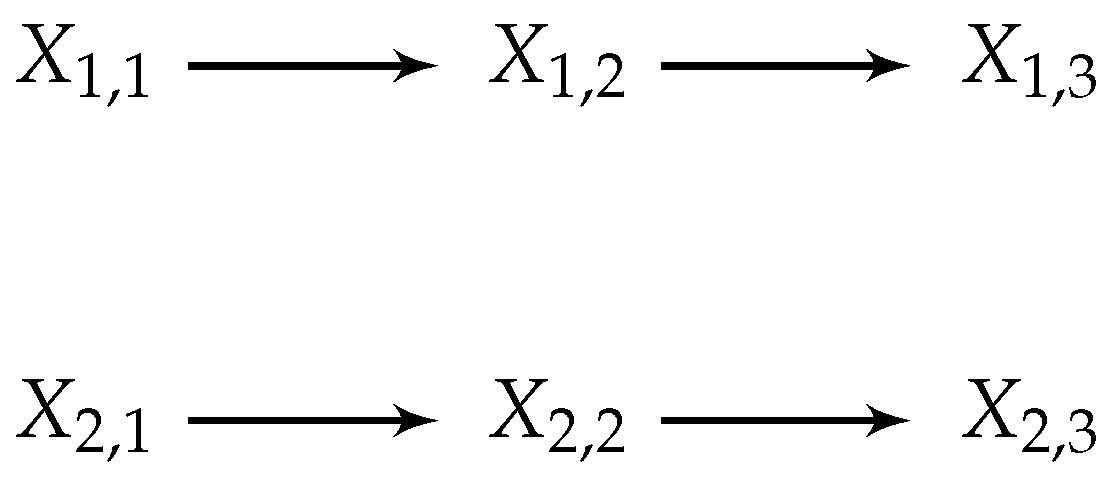
4.2. Two Constant and Independent Binary Random Variables: M C =

4.2.1. Definition

Define the time- and space-homogeneous multivariate Markov chain M C = with Bayesian network { X j , t } j { 1 , 2 } , t { 0 , 1 , 2 } and
pa ( j , t ) = if t = 0 , { ( j , t 1 ) } else ,
p j , t ( x j , t | x j , t 1 ) = δ x j , t 1 ( x j , t ) = 1 if x j , t = x j , t 1 , 0 else ,
p j , 0 ( x j , 0 ) = 1 / 4 .
The Bayesian network can be seen in Figure 4.

4.2.2. Trajectories

In order to get the disintegration hierarchy D ( x V ) we have to choose a trajectory x V and calculate the SLI of each partition π L ( V ) . There are only four different trajectories possible in M C = and they are:
x V = ( x 1 , 0 , x 2 , 0 , x 1 , 1 , x 2 , 1 , x 1 , 2 , x 2 , 2 ) = ( 0 , 0 , 0 , 0 , 0 , 0 ) if x 1 , 0 = 0 , x 2 , 0 = 0 ; ( 0 , 1 , 0 , 1 , 0 , 1 ) if x 1 , 0 = 0 , x 2 , 0 = 1 ; ( 1 , 0 , 1 , 0 , 1 , 0 ) if x 1 , 0 = 1 , x 2 , 0 = 0 ; ( 1 , 1 , 1 , 1 , 1 , 1 ) if x 1 , 0 = 1 , x 2 , 0 = 1 .
Each of these trajectories has probability p V ( x V ) = 1 / 4 and all other trajectories have p V ( x V ) = 0 . We call the four trajectories the possible trajectories. We visualise the possible trajectories as a grid with each cell corresponding to one variable. The spatial indices are constant across rows and time-slices V t correspond to the columns. A white cell indicates a 0 and a black cell indicates a 1. This results in the grids of Figure 5.

4.2.3. Partitions of Trajectories

The disintegration hierarchy is composed out of all partitions in the lattice of partitions L ( V ) . Recall that we are partitioning the entire spatially and temporally extended index set V of the Bayesian network and not only the time-slices. Blocks in the partitions of L ( V ) are then, in general, spatiotemporally and not only spatially extended patterns.
The number of partitions | L ( V ) | of a set of | V | = 6 elements is B 6 = 203 ( B n is the Bell number of n). These partitions π can be classified according to their cardinality | π | (number of blocks in the partition). The number of partitions of a set of cardinality | V | into | π | blocks is the Stirling number ( | V | , | π | ) . For | V | = 6 we find the Stirling numbers:
Entropy 19 00230 i002
It is important to note that the partition lattice L ( V ) is the same for all trajectories as it is composed out of partitions of V. On the other hand the values of SLI mi π ( x V ) with respect to the partitions in L ( V ) generally depend on the trajectory x V .

4.2.4. SLI Values of the Partitions

We can calculate the SLI mi π ( x V ) of every trajectory x V with respect to each partition π L ( V ) according to Definition 5:
mi π ( x V ) : = log p V ( x V ) b π p b ( x b ) .
In the case of M C = the SLI values with respect to each partition do not depend on the trajectories. For an overview we plotted the values of SLI with respect to each partition π L ( V ) for any trajectory of M C = in Figure 6.
We can see in Figure 6 that the cardinality does not determine the value of SLI. At the same time there seems to be a trend to higher values of SLI with increasing cardinality of the partition. We can also observe that only five different values of SLI are attained by partitions on this trajectory. We will collect these classes of partitions with equal SLI values in the disintegration hierarchy next.

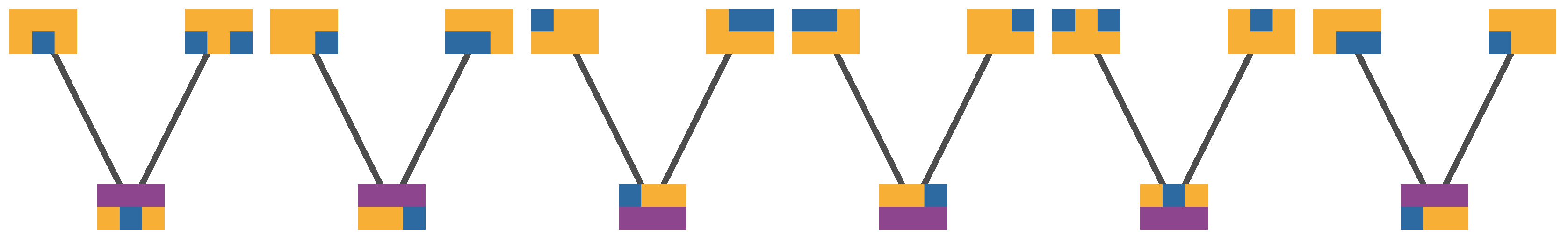
4.2.5. Disintegration Hierarchy

In order to get insight into the internal structure of the partitions of a trajectory x V we obtain the disintegration hierarchy D ( x V ) (see Definition 10) and look at the Hasse diagrams of each of the disintegration levels D i ( x V ) partially ordered by refinement. If we sort the partitions of any trajectory of M C = according to increasing SLI value we obtain Figure 7. There we see groups of partitions attaining the SLI values { 0 , 1 , 2 , 3 , 4 } (precisely) these groups are the disintegration levels { D 1 ( x V ) , D 2 ( x V ) , D 3 ( x V ) , D 4 ( x V ) , D 5 ( x V ) } . The exact numbers of partitions in each of the levels are:
Entropy 19 00230 i003
Next we look at the Hasse diagram of each of those disintegration levels. Since the disintegration levels are subsets of the partition lattice L ( V ) , they are in general not lattices by themselves. The Hasse diagrams (see Appendix B for the definition) visualise the set of partitions in each disintegration level partially ordered by refinement ⊲ . The Hasse diagrams are shown in Figure 8. We see immediately that within each disintegration level apart from the first and the last the Hasse diagrams contain multiple connected components.
Furthermore, within a disintegration level the connected components often have the same Hasse diagrams. For example, in D 2 (Figure 8b) we find six connected components with three partitions each. The identical refinement structure of the connected components is related to the symmetries of the probability distribution over the trajectories. As it requires further notational overhead and is straightforward we do not describe these symmetry properties formally. In order to see the symmetries, however, we visualise the partitions themselves in the Hasse diagrams in Figure 9. We also visualise examples of the different connected components in each disintegration level in Figure 10.
Recall that due to the disintegration theorem (Theorem 6) we are interested especially in partitions that do not have refinements at their own or any preceding (i.e., lower indexed) disintegration level. These partitions consist of blocks that are completely integrated. i.e., all possible partitions of each of the blocks results in a positive SLI value or is a single node of the Bayesian network. The refinement-free disintegration hierarchy D ( x V ) contains only these partitions and is shown in a Hasse diagram in Figure 11.

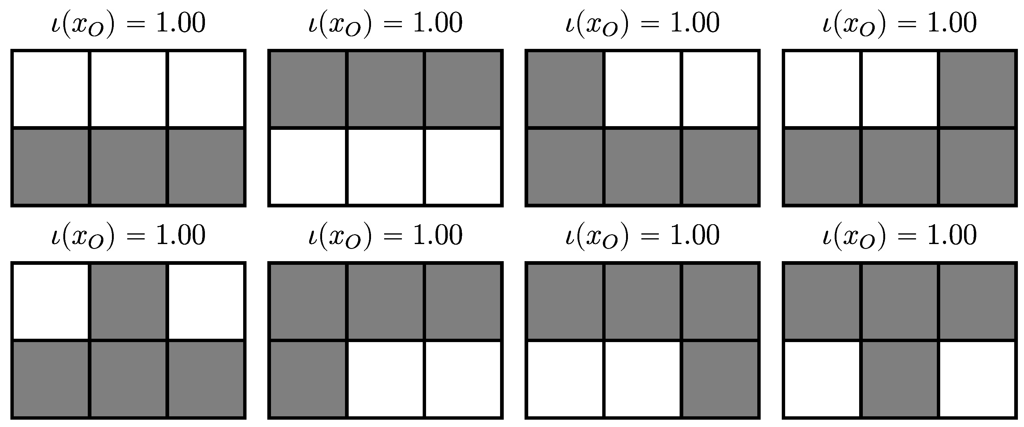
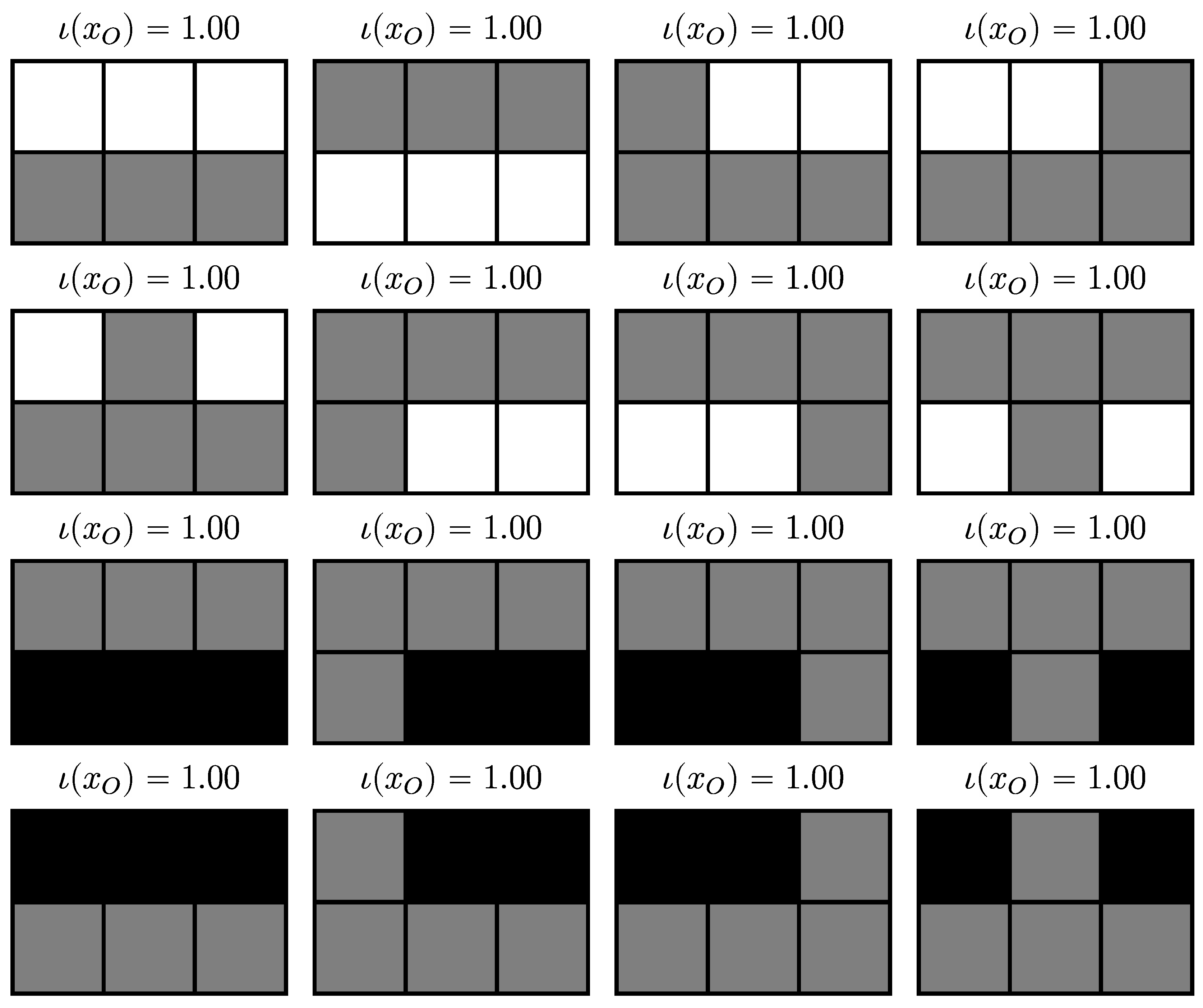
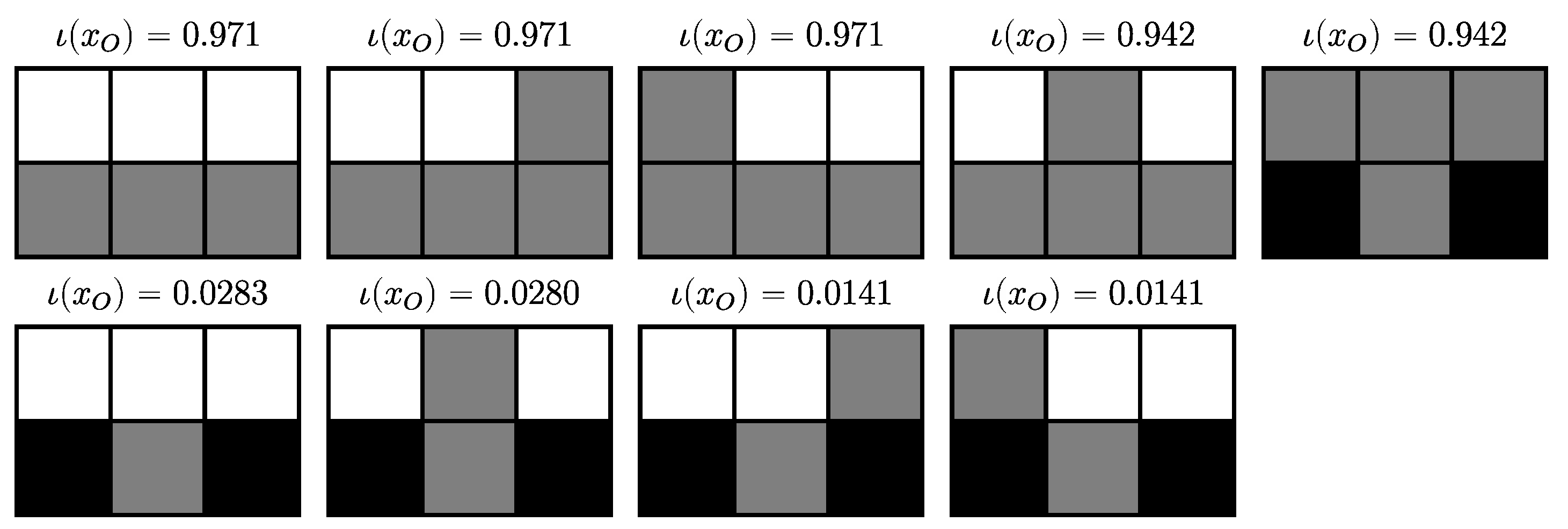
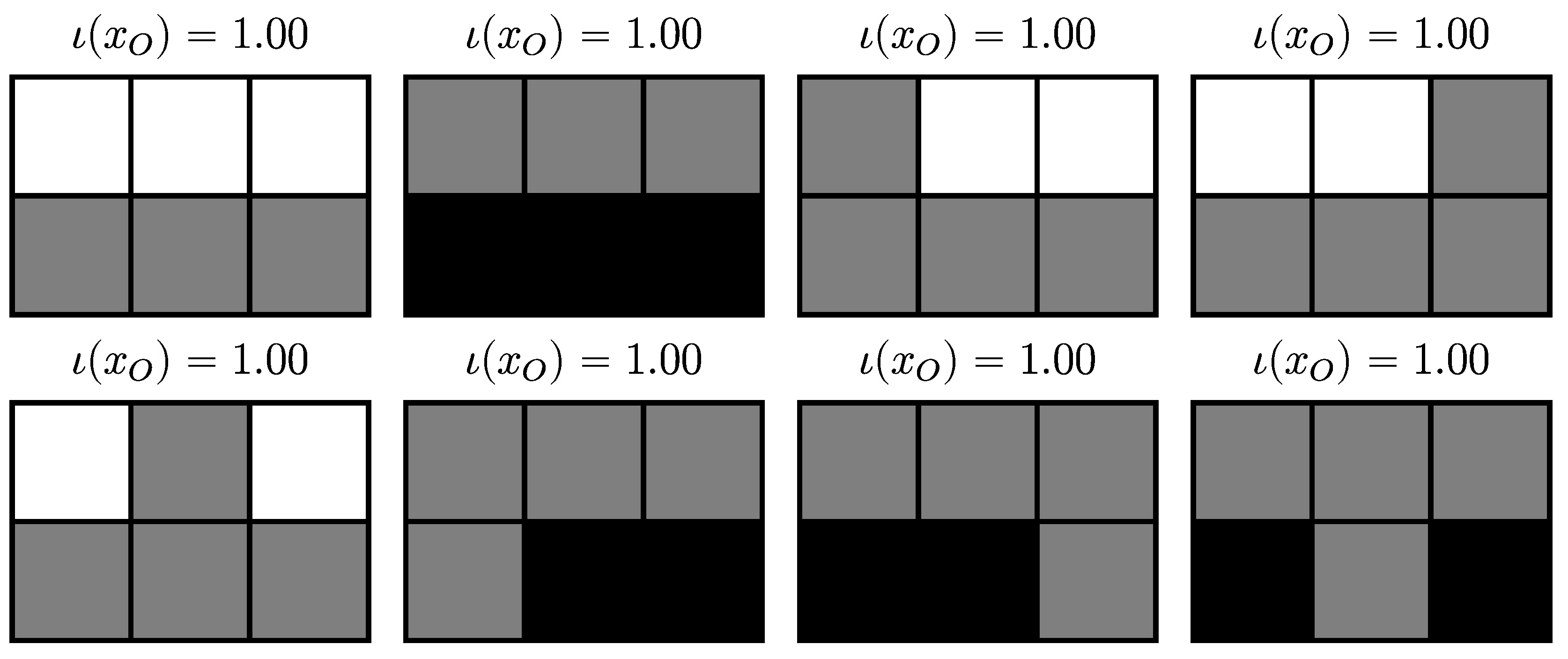
4.2.6. Completely Integrated Patterns

Having looked at the disintegration hierarchy we now make use of it by extracting the completely (When it is clear from context that we are talking about complete local integration we drop “local” for the sake of readability.) integrated patterns ( ι -entities) of the four trajectories of M C = . Recall that due to the disintegration theorem (Theorem 6) we know that all blocks in partitions that occur in the refinement-free disintegration hierarchy are either singletons or correspond to ι -entities. If we look at the refinement-free disintegration hierarchy in Figure 11 we see that many blocks occur in multiple partitions and across disintegration levels. We also see that there are multiple blocks that are singletons. If we ignore singletons, which are trivially integrated as they cannot be partitioned, we end up with eight different blocks. Since the disintegration hierarchy is the same for all four possible trajectories these blocks are also the same for each of them (note that this is the case for M C = but not in general as we will see in Section 4.3). However, the patterns that result are different due to the different values within the blocks. We show the eight ι -entities and their complete local integration (Definition 6) on the first trajectory in Figure 12 and on the second trajectory in Figure 13.
Since the disintegration hierarchies are the same for the four possible trajectories of M C = we get the same refinement-free partitions and therefore the same blocks containing the ι -entities. This is apparent when comparing Figure 12 and Figure 13 and noting that each pattern occurring on the first trajectory has a corresponding pattern on the second trajectory that differs (if at all) only in the values of the cells it fixes and not in what values it fixes. More visually speaking, for each pattern in Figure 12 there is a corresponding pattern in Figure 13 leaving the same cells grey.
If we are not interested in a particular trajectory, we can also look at all different ι -entities on any trajectory. For M C = these are shown in Figure 14.
We see that all ι -entities x O have the same value of complete local integration ι ( x O ) = 1 . This can be explained using the deterministic expression for the SLI of Equation (30) and noting that for M C = if any of the values x j , t is fixed by a pattern then ( x j , s ) s T = x j , T are determined since they must be the same value. This means that the number of trajectories N ( x j , S ) in which any pattern x j , S with S T occurs is either N ( x j , S ) = 0 , if the pattern is impossible, or N ( x j , S ) = 2 since there are two trajectories compatible with it. Note that all blocks x b in any of the ι -entities and all ι -entities x O themselves are of the form x j , S with S T . Let N ( x j , S ) = : N and plug this into Equation (30) for an arbitrary partition π :
mi π ( x O ) = ( | π | 1 ) log | X V 0 | log b π N ( x b ) N ( x O )
= ( | π | 1 ) log | X V 0 | log N | π | N
= ( | π | 1 ) log | X V 0 | N .
To get the complete local integration value we have to minimise this with respect to π where | π | 2 . So for | X V 0 | = 4 and N = 2 we get ι ( x O ) = 1 .
Another observation is that the ι -entities are all limited to one of the two rows. This shows on a simple example that, as we would expect, ι -entities cannot extend from one independent process to another.

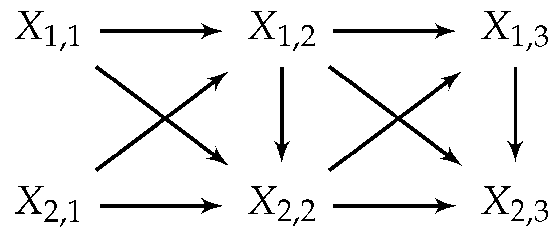
4.3. Two Random Variables with Small Interactions

In this section we look at a system almost identical to that of Section 4.2 but with a kind of noise introduced. This allows all trajectories to occur and is designed to test whether the spatiotemporal patterns maintain integration in the face of noise.

4.3.1. Definition

We define the time- and space-homogeneous multivariate Markov chain M C ϵ via the Markov matrix P with entries
P f ( x 1 , t + 1 , x 2 , t + 1 ) , f ( x 1 , t , x 2 , t ) = p J , t + 1 ( x 1 , t + 1 , x 2 , t + 1 | x 1 , t , x 2 , t )
where we define the function f : { 0 , 1 } 2 [ 1 : 4 ] via
f ( 0 , 0 ) = 1 , f ( 0 , 1 ) = 2 , f ( 1 , 0 ) = 3 , f ( 1 , 1 ) = 4 .
With this convention P is
P = 1 3 ϵ ϵ ϵ ϵ ϵ 1 3 ϵ ϵ ϵ ϵ ϵ 1 3 ϵ ϵ ϵ ϵ ϵ 1 3 ϵ
This means that the state of both random variables remains the same with probability 1 3 ϵ and transitions into each of the other possible combinations with probability ϵ . The noise then does not act independently on both random variables but disturbs the joint state. This makes ι -entities possible that extend across the two processes. In the following we set ϵ = 1 / 100 . The initial distribution is again the uniform distribution
p j , 0 ( x j , 0 ) = 1 / 4 .
Writing this multivariate Markov chain as a Bayesian network is possible but the conversion is tedious. The Bayesian network one obtains can be seen in Figure 15.

4.3.2. Trajectories

In this system all trajectories are possible trajectories. This means there are 2 6 = 64 possible trajectories, since every one of the six random variables can be in any of its two states. There are three classes of trajectories with equal probability of occurring. The first class with the highest probability of occurring are the four possible trajectories of M C = . Then there are 24 trajectories that make a single ϵ -transition (i.e., a transition where the next pair is not the same as the current one ( x 1 , t + 1 , x 2 , t + 1 ) ( x 1 , t , x 2 , t ) , these transitions occur with probability ϵ ), and 36 trajectories with two ϵ -transitions. We pick only one trajectory from each class. The representative trajectories are shown in Figure 16 and will be denoted x V 1 , x V 2 , and x V 3 respectively. The probabilities are p V ( x V 1 ) = 0.235225 , p V ( x V 2 ) = 0.0024250 , p V ( x V 3 ) = 0.000025 .

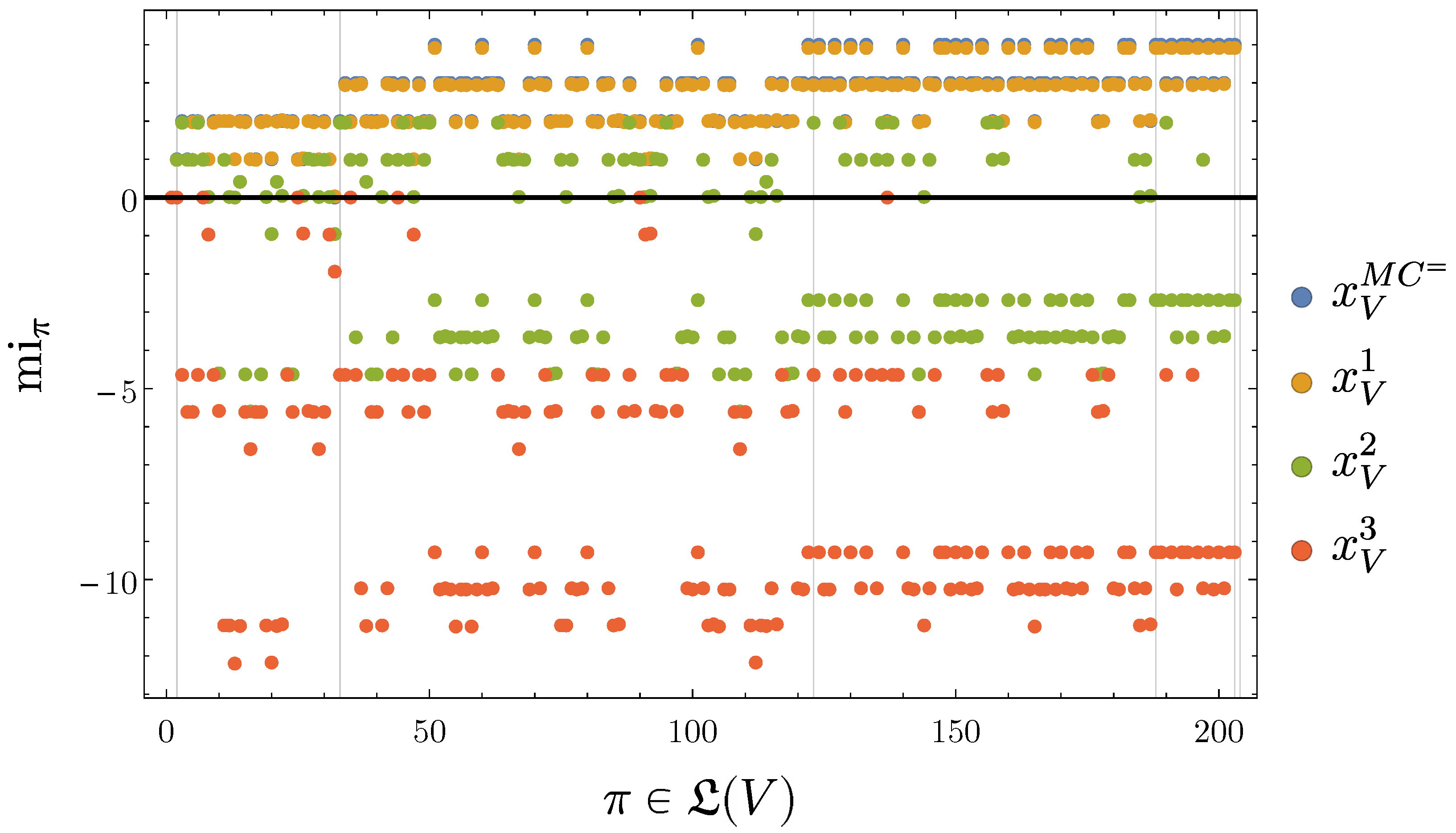
4.3.3. SLI Values of the Partitions

Again we calculate the SLI mi π ( x V ) of every trajectory x V with respect to each partition π L ( V ) . In contrast to M C = the SLI values with respect to each partition of M C ϵ do depend on the trajectories. We plot the values of SLI with respect to each partition π L ( V ) for the three representative trajectories in Figure 17.
It turns out that the SLI values of x V 1 are almost the same as those of M C = in Figure 6 with small deviations due to the noise. This should be expected as x V 1 is also a possible trajectory of M C = . Also note that trajectories x V 2 , x V 3 exhibit negative SLI with respect to some partitions. In particular, x V 3 has non-positive SLI values with respect to any partition. This is due to the low probability of this trajectory compared to its parts. The blocks of any partition have so much higher probability than the entire trajectory that the product of their probabilities is still greater or equal to the trajectory probability.

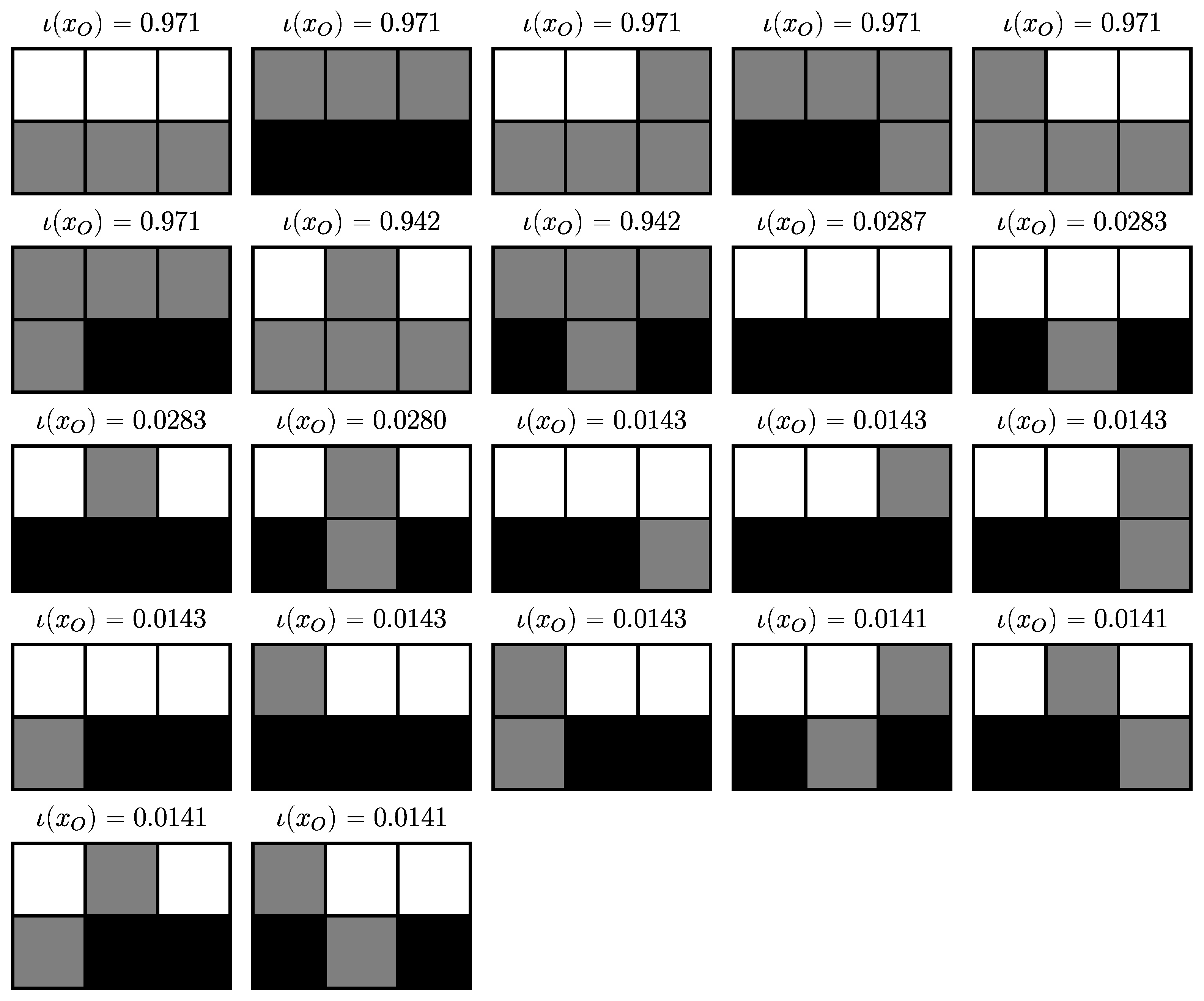
4.3.4. Completely Integrated Patterns

In this section we look at the ι -entities for each of the three representative trajectories x V k , k { 1 , 2 , 3 } . They are visualised together with their complete local integration values in Figure 18, Figure 19 and Figure 20. In contrast to the situation of M C = we now have ι -entities with varying values of complete local integration.
On the first trajectory x V 1 we find all the eight patterns that are completely locally integrated in M C = (see Figure 13). These are also more than an order of magnitude more integrated than the rest of the ι -entities. This is also true for the other two trajectories.

5. Discussion

In Section 3.1 we have argued for the use of patterns as candidates for entities. Patterns can be composed of arbitrary spatially and temporally extended parts of trajectories. We have seen in Theorem 1 that they are distinct from arbitrary subsets of trajectories. The important insight here is that patterns are structures that occur within trajectories but this cannot be said of sets of trajectories.
One of the main target applications of patterns is in time-unrolled Bayesian networks of cellular automata like those in Figure 1. Patterns in such Bayesian networks become spatiotemporal patterns like those used to describe the glider, block, and blinker in the Game of Life cellular automaton by Beer [14]. We would also like to investigate whether the latter spatiotemporal patterns are ι -entities. However, at the present state of the computational models and, without approximations, this was out of reach computationally. We will discuss this further below.
In Section 3.3 we defined SLI and in Section 3.3 gave its expression for deterministic Bayesian networks (including cellular automata) as well. We also established the least upper bound of SLI with respect to a partition π of cardinality n for a pattern x A with probability q. This upper bound is achieved if each of the blocks x b in the partition π occur if and only if the whole pattern x O occurs. This is compatible with our interpretation of entities since in this case clearly the occurrence of any part of the pattern leads necessarily to the occurrence of the entire pattern (and not only vice versa).
We also presented a candidate for a greatest lower bound of SLI with respect to a partition of cardinality n for a pattern with probability q. Whether this is the greatest lower bound or not it shows a case for which SLI is always negative. This happens if either the whole pattern x A occurs (with probability q) or one of the “almost equal” patterns occurs, each with identical probability. A pattern y A is almost equal to x A with respect to π in this sense if it only differs at one of the blocks b π i.e., if y A = ( x A \ b , z b ) where z b x b . This construction makes as many parts as possible (i.e., all but one) occur as many times as possible without the whole pattern occurring. This creates large marginalised probabilities p b ( x b ) for each part/block which means that their product probability also becomes large.
Beyond these quantitative interpretations an interpretation of the greatest lower bound candidate seems difficult. A more intuitive candidate for the opposite of an integrated pattern seem to be patterns with independent parts. i.e., zero SLI but quantitatively these are not on the opposite end of the SLI spectrum. A more satisfying interpretation of the presented candidate is still to be found.
We also proved the disintegration theorem which relates states that the refinement-free partitions of a trajectory among those partitions achieving a particular SLI value consist of ι -entities only, where an ι -entity is a pattern with positive CLI. This theorem allows us to interpret the ι -entities in new ways and may lead to a more formal or quantitative justification of ι -entities. It is already a first step in this direction since it establishes a special role of the ι -entities within trajectories of Bayesian networks. A further justification would tell us what in turn the refinement-free partitions can be used for. We have discussed a possible direction for further investigation in detail in Section 3.5. This tried to connect the ι -entities with a coding problem.
In Section 4 we investigated SLI and CLI in three simple example sets of random variables. We found that if the random variables are all independently distributed the according entities are just all the possible x j X j of each of the random variables X j { X i } i V . This is what we would expect from an entity criterion. There are no entities with any further extent than a single random variable and each value corresponds to a different entity.
For the simple Markov chain M C = composed out of two independent and constant processes we presented the entire disintegration hierarchy and the Hasse diagrams of each disintegration level ordered by refinement. The Hasse diagrams reflected the highly symmetric dynamics of the Markov chain via multiple identical components. For the refinement-free disintegration hierarchy we then get multiple partitions at the same disintegration level as well. Different partitions of the trajectory imply overlapping blocks which in the case of the refinement-free partition are ι -entities. So in general the ι -entities at a particular disintegration level are not necessarily unique and can overlap. We also saw in Figure 11 that the same ι -entities can occur on multiple disintegration levels.
The ι -entities of M C = included the expected three timestep constant patterns within each of the two independent processes. It also included the two timestep parts of these constant patterns. This may be less expected. It shows that parts of ι -entities can be ι -entities themselves. We note that these “sub-entities (those that are parts of larger entities) are always on a different disintegration level than their” super-entities (the larger entities). We can speculate that the existence of such sub- and super-entities on different disintegration levels may find an interpretation through multicellular organisms or similar structures. However, the overly simplistic examples here only serve as basic models for the potential phenomena, but are still far too simplistic to warrant any concrete interpretation in this direction.
We also looked at a version of M C = perturbed by noise, denoted M C ϵ . We found that the entities of M C = remain the most strongly integrated entities in M C ϵ . At the same time new entities occur. So we observe that in M C ϵ the entities vary from one trajectory to another (Figure 18, Figure 19 and Figure 20). We also observe spatially extended entities i.e., entities that extend across both (formerly independent) processes. We also observe entities that switch from one process to the other (from top row to bottom row or vice versa). The capacity of entities to exhibit this behaviour may be necessary to capture the movement or metabolism of entities in more realistic scenarios. In Biehl et al. [8] we argued that these properties are important and showed that they hold for a crude approximation of CLI (namely for SLI with respect to π = 0 ) but not for the full CLI measure.
We established that the ι -entities:
  • correspond to fixed single random variables for a set of independent random variables,
  • can vary from one trajectory to another,
  • and can change the degrees of freedom that they occupy over time,
  • can be ambiguous at a fixed level of disintegration due to symmetries of the system,
  • can overlap at the same level of disintegration due to this ambiguity,
  • can overlap across multiple levels of disintegration i.e., parts of ι -entities can be ι -entities again.
In general the examples we investigated concretely are too small to sufficiently support the concept of positive CLI as an entity criterion. Due to the extreme computational burden, this may remain the case for a while. For a straightforward calculation of the minimum SLI of a trajectory of a Bayesian network { X i } i V with | V | = k nodes we have to calculate the SLI with respect to B k partitions. According to (Bruijn [43], p. 108) the Bell numbers B n grow super-exponentially. Furthermore, to evaluate the SLI we need the joint probability distribution of the Bayesian network { X i } i V . Naively, this means we need the probability (a real number between 0 and 1) of each trajectory. If we only have binary random variables, the number of trajectories is 2 | V | which make the straightforward computation of disintegration hierarchies unrealistic even for quite small systems. If we take a seven by seven grid of the game of life cellular automaton and want to look at three time-steps we have | V | = 147 . If we use 32 bit floating numbers this gives us around 10 30 petabytes of storage needed for this probability distribution. We are sceptical that the exact evaluation of reasonably large systems can be achieved even with non-naive methods. This suggests that formal proofs may be the more promising way to investigate SLI and CLI further.

Acknowledgments

Part of the research was performed during Martin Biehl’s time as a JSPS International Research Fellow and as an ELSI Origins Network (EON) long term visitor. Daniel Polani was supported in part by the EC Horizon 2020 H2020-641321 socSMCs FET Proactive project.

Author Contributions

Martin Biehl, Takashi Ikegami, and Daniel Polani conceived the problem and the measures, and wrote the paper; Martin Biehl proved the theorems and conceived and calculated the examples. All authors have read and approved the final manuscript.

Conflicts of Interest

The authors declare no conflict of interest.

Abbreviations

The following abbreviations are used in this manuscript:
SLISpecific local integration
CLIComplete local integration

Appendix A. Kronecker Delta

The Kronecker–delta is used in this paper to represent deterministic conditional distributions.
Definition A1 (Delta).
Let X be a random variable with state space X then for x X and a subset C X define
δ x ( C ) : = 1 if x C , 0 else .
We will abuse this notation if C is a singleton set C = { x ¯ } by writing
δ x ( x ¯ ) : = 1 if x { x ¯ } , 0 else .
= 1 if x = x ¯ , 0 else .
The second line is a more common definition of the Kronecker–delta.
Remark:
  • Let X , Y be two random variables with state spaces X , Y and f : X Y a function such that
    p ( y | x ) = δ f ( x ) ( y ) ,
    then
    p ( y ) = x p Y ( y | x ) p X ( x )
    = x δ f ( x ) ( y ) p X ( x )
    = x δ x ( f 1 ( y ) ) p X ( x )
    = x f 1 ( y ) p X ( x )
    = p X ( f 1 ( y ) ) .

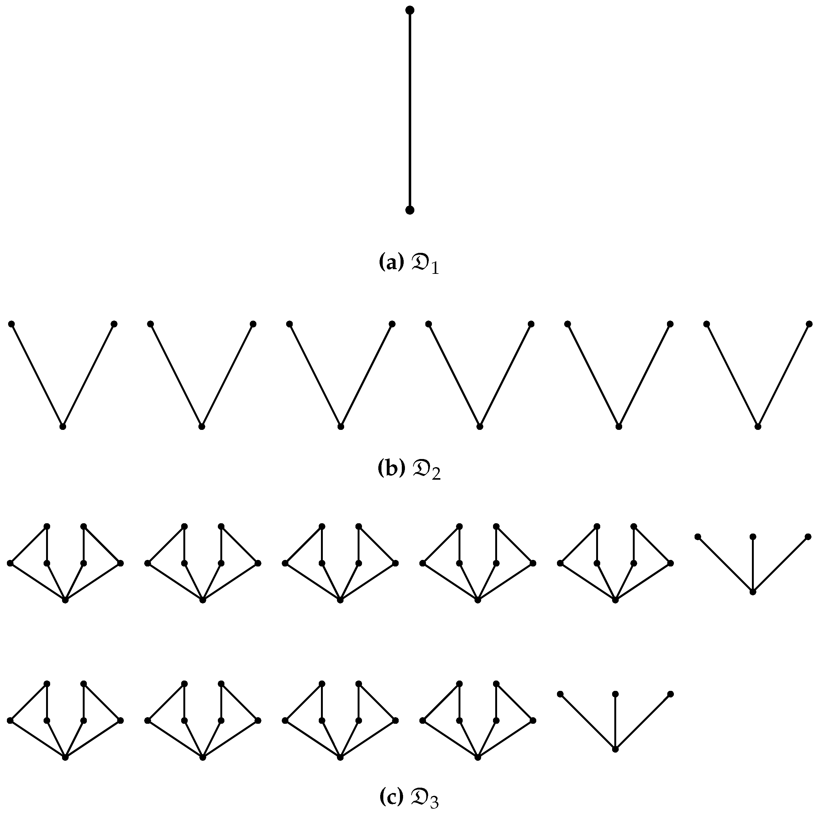
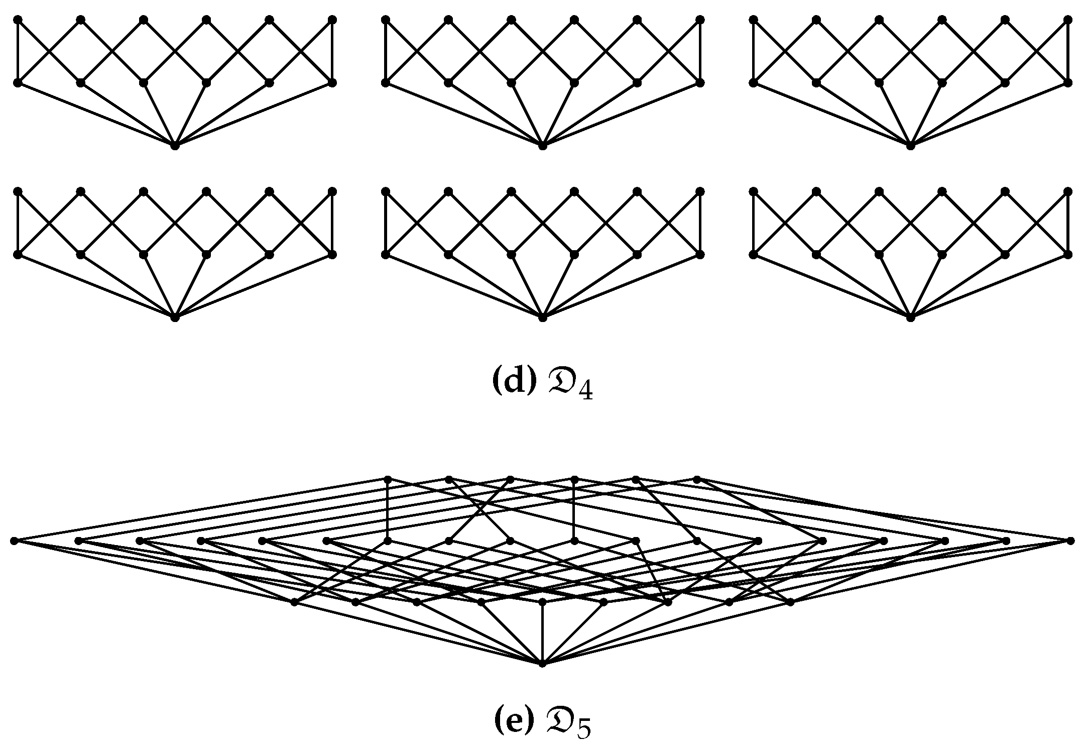
Appendix B. Refinement and Partition Lattice Examples

This appendix recalls the definitions of set partitions, refinement and coarsening of set partitions, and Hasse diagrams. It also shows the Hasse diagram of an example partition lattices. The definitions are due to Grätzer [28].
Definition A2.
A (set) partition π of a set X is a set of non-empty subsets (called blocks ) of X satisfying
1. 
for all x 1 , x 2 π , if x 1 x 2 , then x 1 x 2 = ,
2. 
x π = X .
We write L ( X ) for the set of all partitions of X .
Remark:
  • In words, a partition of a set is a set of disjoint non-empty subsets whose union is the whole set.
Definition A3.
If two elements x 1 , x 2 X belong to the same block of a partition π of X write x 1 π x 2 . Also write x 1 / π for the block { x 2 X : x 2 π x 1 } .
Definition A4 (Refinement and coarsening).
We define the binary relationbetween partitions π , ρ L ( X ) as:
π ρ if x 1 π x 2 implies x 1 ρ x 2 .
In this case π is called a refinement of ρ and ρ is called a coarsening of π.
Remarks:
  • More intuitively, π is a refinement of ρ if all blocks of π can be obtained by further partitioning the blocks of ρ . Conversely, ρ is a coarsening of π if all blocks in ρ are unions of blocks in π .
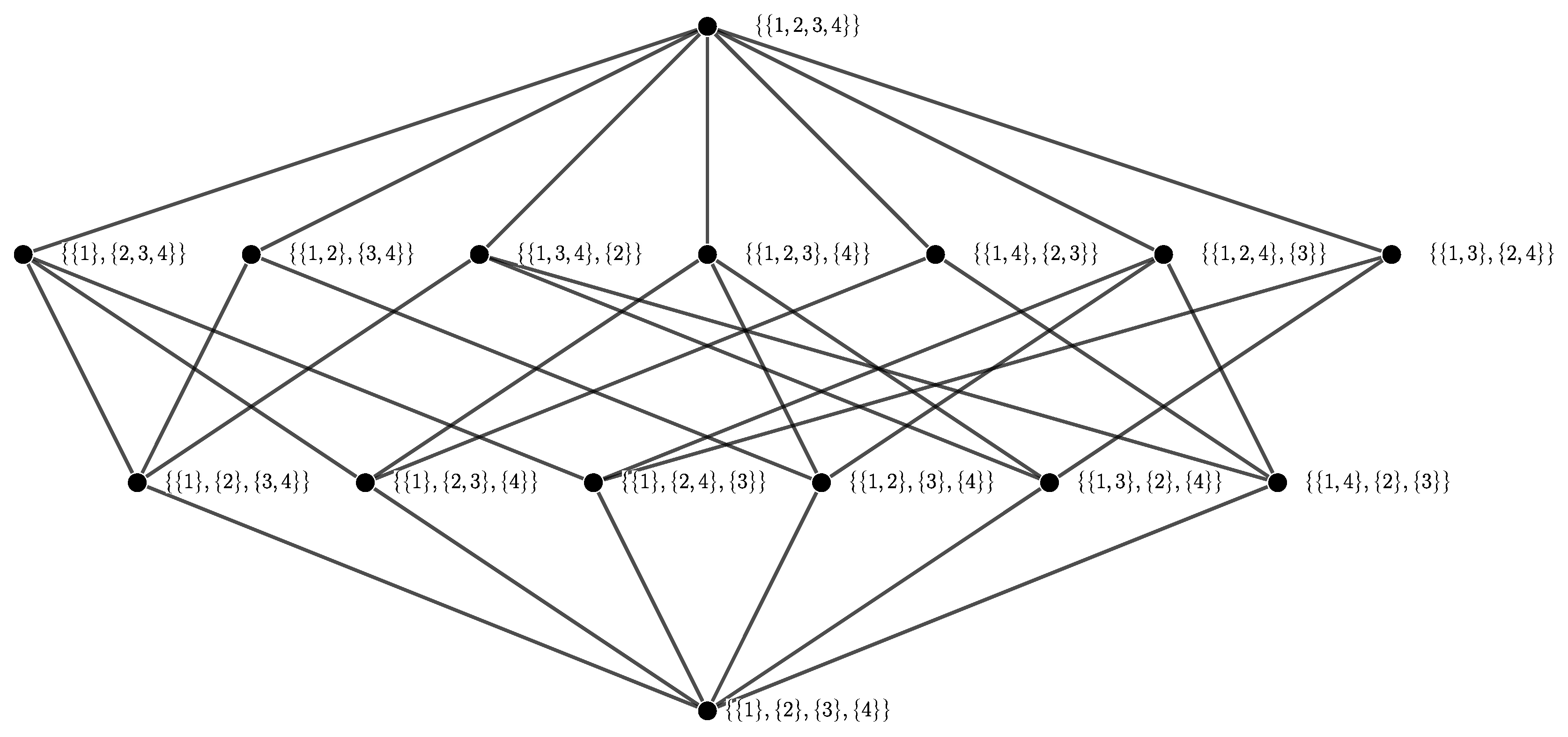
  • Examples are contained in the Hasse diagrams (defined below) shown in Figure A1.
Definition A5 (Hasse diagram).
A Hasse diagram is a visualisation of a poset (including lattices). Given a poset A ordered bythe Hasse diagram represents the elements of A by dots. The dots representing the elements are arranged in such a way that if a , b A , a b , and a b then the dot representing a is drawn below the dot representing b. An edge is drawn between two elements a , b A if a : b , i.e., if b covers a. If edges cross in the diagram this does not mean that there is an element of A where they cross and edges never pass through a dot representing an element.
Remarks:
  • No edge is drawn between two elements a , b A if a b but not a : b .
  • Only drawing edges for the covering relation does not imply a loss of information about the poset since the covering relation determines the partial order completely.
  • For an example Hasse diagrams see Figure A1.
Figure A1. Hasse diagrams of the partition lattice of the four element set.
Entropy 19 00230 g021

Appendix C. Bayesian Networks

Intuitively a Bayesian network is a graph representation of the inter-dependencies of a set of random variables. Recall that any joint probability distribution over a set { X i } i I with I = { 1 , . . . , n } of random variables can always be written as a product of conditional probabilities:
p I ( x 1 , . . . , x n ) = i = 1 n 1 p i ( x i | x i + 1 , . . . , x n ) p ( x n ) .
This also holds for any reordering of the indices i f ( i ) with f : { 1 , . . . n } { 1 , . . . n } bijective.
In many cases however this factorisation can be simplified. Often some of the conditional probabilities p ( x i | x i + 1 , . . . , x n ) do not depend on all variables { x i + 1 , . . . , x n } listed in the product of Equation (A11). For example, X 1 might only depend on X 2 so we would have p ( x 1 | x 2 , . . . , x n ) = p ( x 1 | x 2 ) . Note that the latter conditional probability is determined by fixing | X 2 | ( | X 1 | 1 ) probabilities whereas the former needs i = 1 n | X i + 1 | ( | X 1 | 1 ) probabilities to be fixed. This means the number of parameters (the probabilities) of the joint distribution p ( x 1 , . . . , x n ) is often much smaller than suggested by Equation (A11). One way to encode this simplification and make sure that we are dealing only with joint probabilities that reflect the dependencies we allow are Bayesian networks. These can be defined as follows. First we define graphs that are factorisation compatible with joint probability distributions over a set of random variables and then define the Bayesian networks as pairs of joint probability distributions and a factorisation compatible graph.
Definition A6.
A directed acyclic graph G = ( V , E ) with nodes V and edges E is factorisation compatible with the joint probabilities the probabilities of a probability distribution p V : X V [ 0 , 1 ] iff the latter can be factorised in the way suggested by G which means:
p V ( x V ) = i V p ( x i | x pa ( i ) ) .
where pa ( i ) denotes the parents of node i according to G.
Remark:
  • In general there are multiple directed acyclic graphs that are factorisation compatible with the same probability distribution. For example, if we choose any total order for the nodes in V and define a graph by pa ( i ) = { j V : j < i } then Equation (A12) becomes Equation (A11) which always holds.
Definition A7 (Bayesian network).
A Bayesian network is a (here assumed finite) set of random variables { X i } i V and a directed acyclic graph G = ( V , E ) with nodes indexed by V such that the joint probability distribution p V : X V [ 0 , 1 ] of { X i } i V is factorisation compatible with G. We also refer to the graph set of random variables { X i } i V as a Bayesian network implying the graph G.
Remarks:
  • On top of constituting the vertices of the graph G the set V is also assumed to be totally ordered in an (arbitrarily) fixed way. Whenever we use a subset A V to index a sequence of variables in the Bayesian network (e.g., in p A ( x A ) ) we order A according to this total order as well.
  • Since { X i } i V is finite and G is acyclic there is a set V 0 of nodes without parents.
Definition A8 (Mechanism).
Given a Bayesian network { X i } i V with index set V for each node with parents i.e., for each node i V \ V 0 (with V 0 the set of nodes without parents) the mechanism of node i or also called the mechanism of random variable X i is the conditional probability (also called a transition kernel) p i : X pa ( i ) × X i [ 0 , 1 ] mapping ( x pa ( i ) , x i ) p i ( x i | x pa ( i ) ) . For each x pa ( i ) the mechanism defines a probability distribution p i ( . | x pa ( i ) ) : X i [ 0 , 1 ] satisfying (like any other probability distribution)
x i X i p i ( x i | x pa ( i ) ) = 1 .
Remarks:
  • We could define the set of all mechanisms to formally also include the mechanisms of the nodes without parents V 0 . However, in practice it makes sense to separate the nodes without parents as those that we choose an initial probability distribution over (similar to a boundary condition) which is then turned into a probability distribution p V over the entire Bayesian network { X i } i V via Equation (A12). Note that in Equation (A12) the nodes in V 0 are not explicit as they are just factors p i ( x i | x pa ( i ) ) with pa ( i ) = .
  • To construct a Bayesian network, take graph G = ( V , E ) and equip each node i ( V \ V 0 ) with a mechanism p i : X pa ( i ) × X i [ 0 , 1 ] and for each node i V 0 choose a probability distribution p i : X i [ 0 , 1 ] . The joint probability distribution is then calculated by the according version of Equation (A12):
    p V ( x V ) = i V \ V 0 p i ( x i | x pa ( i ) ) j V 0 p j ( x j ) .

Appendix C.1. Deterministic Bayesian Networks

Definition A9 (Deterministic mechanism).
A mechanism p i : X pa ( i ) × X i [ 0 , 1 ] is deterministic if there is a function f i : X pa ( i ) X i such that
p i ( x i | x pa ( i ) ) = δ f i ( x pa ( i ) ) ( x i ) = 1 i f x i = f i ( x pa ( i ) ) , 0 e l s e .
Definition A10 (Deterministic Bayesian network).
A Bayesian network { X i } i V is deterministic if all its mechanisms are deterministic.
Theorem A1.
Given a deterministic Bayesian network { X i } i V there exists a function f V \ V 0 : X V 0 X V \ V 0 which given a value x V 0 of the random variables without parents X V 0 returns the value x V \ V 0 fixing the values of all remaining random variables in the network.
Proof. 
According to Equation (A12), the definition of conditional probabilities, and using the deterministic mechanisms we have:
p V \ V 0 ( x V \ V 0 | x V 0 ) = i V \ V 0 p i ( x i | x pa ( i ) )
= i V \ V 0 δ f i ( x pa ( i ) ) ( x i ) .
For every x V 0 the product on the right hand side is a probability distribution and therefore is always greater or equal to zero and maximally one. Also for every x V 0 the sum of the probabilities over all x V \ V 0 X V \ V 0 is equal to one. As a product of zeros and/or ones the right hand side on the second line can only either be zero or one. This means for every x V 0 there must be a unique x V \ V 0 such that the right hand side is equal to one. Define this as the value of the function f V \ V 0 ( x V 0 ) . ☐
Theorem A2 (Pattern probability in a deterministic Bayesian network).
Given a deterministic Bayesian network (Definition A10) and uniform initial distribution p V 0 : X V 0 [ 0 , 1 ] the probability of the occurrence of a pattern x A is:
p A ( x A ) = N ( x A ) | X V 0 |
where N ( x A ) is the number of trajectories x ¯ V in which x A occurs.
Proof. 
Recall that in a deterministic Bayesian network we have a function f V \ V 0 : X V 0 X V \ V 0 (see Theorem A1) which maps a given value of x V 0 to the value of the rest of the network x V \ V 0 . We calculate p A ( x A ) for an arbitrary subset A V . To make this more readable let A V 0 = A 0 , A \ V 0 = A r , B : = V \ A , B V 0 = B 0 , and B \ V 0 = B r . Then
p A ( x A ) = x ¯ B p V ( x A , x ¯ B )
= x ¯ B 0 , x ¯ B r p V ( x A r , x ¯ B r | x A 0 , x ¯ B 0 ) p V 0 ( x A 0 , x ¯ B 0 )
= x ¯ B 0 , x ¯ B r δ f V \ V 0 ( x A 0 , x ¯ B 0 ) ( x A r , x ¯ B r ) p V 0 ( x A 0 , x ¯ B 0 )
= x ¯ B r { x ¯ B 0 : ( x A 0 , x ¯ B 0 ) f V \ V 0 1 ( x A r , x ¯ B r ) } p V 0 ( x A 0 , x ¯ B 0 )
= 1 | X V 0 | x ¯ B r | { x ¯ B 0 X B 0 : ( x A 0 , x ¯ B 0 ) f V \ V 0 1 ( x A r , x ¯ B r ) } |
= 1 | X V 0 | N ( x A )
In the second to last line we used the uniformity of the initial distribution p V 0 . The second sum in the second to last line counts all initial conditions that are compatible with x A 0 and lead to the occurrence of x A r together with some x ¯ B r . The first one then sums over all such x ¯ B r to get all initial conditions that are compatible with x A 0 and lead to the occurrence of x A r . Together these are all initial conditions compatible with x A . In a deterministic system the number of initial conditions that lead to the occurrence of a pattern x A is equal to the number of trajectories N ( x A ) since every different initial condition will produce a single, unique trajectory. ☐
Remark:
  • Due to the finiteness of the network, deterministic mechanisms, and chosen uniform initial distribution the minimum possible non-zero probability for a pattern x A is 1 / | X V 0 | . This happens for any pattern that only occurs in a single trajectory. Furthermore, the probability of any pattern is a multiple of 1 / | X V 0 | .

Appendix C.2. Proof of Theorem 2

Proof. 
Follows by replacing the probabilities p O ( x O ) and p b ( x b ) in Equation (22) with their deterministic expressions from (Theorem A2), i.e., p A ( x A ) = N ( X A ) / | X V 0 | . Then:
mi π ( x O ) : = log p O ( x O ) b π p b ( x b )
= log N ( x O ) | X V 0 | b π N ( x b ) | X V 0 |
= log N ( x O ) | X V 0 | | X V 0 | | π | b π N ( x b )
= log | X V 0 | | π | 1 N ( x O ) b π N ( x b )
= ( | π | 1 ) log | X V 0 | log b π N ( x b ) N ( x O ) .
 ☐

Appendix D. Proof of Theorem 1

Proof. 
Given a set of random variables { X i } i V , a subset D X V cannot be represented by a pattern of { X i } i V if and only if there exists A V with D A X A (proper subset) and | D A | > 1 , i.e., if neither all patterns at A are possible nor a unique pattern at A is specified by D .
We first show that if there exists A V with D A X A and | D A | > 1 then there is no pattern x ˜ B C V X C with D = T ( x ˜ B ) . Then we show that if no such A exists then there is such a pattern x ˜ B .
Since D A > 1 we have x A , x ¯ A D A X A with x A x ¯ A . Next note that we can write any pattern x ˜ B as
x ˜ B = ( x ˜ B \ A , x ˜ B A ) .
If B A we can see since x ˜ B A must take a single value it cannot contain D since there are trajectories in D taking value x B A on B A and trajectories in D taking values x ¯ B A . More formally, we must have either x ˜ B A = x A or x ˜ B A x A . First, let x ˜ B A = x A but then T ( x ¯ A ) T ( x ˜ B ) so D T ( x ˜ B ) . Next choose x ˜ B A x A but then T ( x A ) T ( x ˜ B ) so also D T ( x ˜ B ) . So we must have B A = .
Now we show that if B A = there are trajectories in x ˜ B that are not in D . We construct one explicitly by fixing its value on A to the value in X A that is not in D A and its value on B to x ˜ B . More formally: choose y A X A \ D A , then y A x A and y A x ¯ A . This is always possible since D A X A (proper subset). Then consider a trajectory x ^ V = ( x ˜ B , y A , x ˇ D ) with arbitrary x ˇ D X D where D = V \ ( B A ) . Then x ^ V T ( x ˜ B ) but x ^ V D .
Conversely, we show how to construct x ˜ B if no such A exists. the idea is just to fix all random variables where | D A | = 1 and leave them unspecified where D A = X A . More formally: if there exists no A V with D A X A and | D A | > 1 , then for each C V either D C = X C or | D C | = 1 . Then let B = { C V : | D C | = 1 } then | D B | = 1 so that we can define x ˜ B as the unique element in D B . Then if y V D we have y B = x ˜ B so D T ( x ˜ B ) . If z V T ( x ˜ B ) we have z B = x ˜ B D B and for A V with A B = by construction of B we have D A = X A such that D V \ B = X V \ B which means z V \ B D V \ B and therefore z V D and T ( x ˜ B ) D . So this gives T ( x ˜ B ) = D . ☐

References

  1. Gallois, A. Identity over Time. In The Stanford Encyclopedia of Philosophy; Zalta, E.N., Ed.; Metaphysics Research Laboratory, Stanford University: Stanford, CA, USA, 2012. [Google Scholar]
  2. Grand, S. Creation: Life and How to Make It; Harvard University Press: Harvard, MA, USA, 2003. [Google Scholar]
  3. Pascal, R.; Pross, A. Stability and its manifestation in the chemical and biological worlds. Chem. Commun. 2015, 51, 16160–16165. [Google Scholar] [CrossRef] [PubMed]
  4. Orseau, L.; Ring, M. Space-Time Embedded Intelligence. In Artificial General Intelligence; Number 7716 in Lecture Notes in Computer Science; Bach, J., Goertzel, B., Iklé, M., Eds.; Springer: Berlin/Heidelberg, Germany, 2012; pp. 209–218. [Google Scholar]
  5. Barandiaran, X.E.; Paolo, E.D.; Rohde, M. Defining Agency: Individuality, Normativity, Asymmetry, and Spatio-temporality in Action. Adapt. Behav. 2009, 17, 367–386. [Google Scholar] [CrossRef]
  6. Legg, S.; Hutter, M. Universal Intelligence: A Definition of Machine Intelligence. arXiv, 2007; arXiv: 0712.3329. [Google Scholar]
  7. Boccara, N.; Nasser, J.; Roger, M. Particlelike structures and their interactions in spatiotemporal patterns generated by one-dimensional deterministic cellular-automaton rules. Phys. Rev. A 1991, 44, 866–875. [Google Scholar] [CrossRef] [PubMed]
  8. Biehl, M.; Ikegami, T.; Polani, D. Towards information based spatiotemporal patterns as a foundation for agent representation in dynamical systems. In Proceedings of the Artificial Life Conference, Cancun, Mexico, 2016; The MIT Press: Cambridge, MA, USA, 2016; pp. 722–729. [Google Scholar]
  9. McGill, W.J. Multivariate information transmission. Psychometrika 1954, 19, 97–116. [Google Scholar] [CrossRef]
  10. Amari, S.I. Information geometry on hierarchy of probability distributions. IEEE Trans. Inf. Theory 2001, 47, 1701–1711. [Google Scholar] [CrossRef]
  11. Lizier, J.T. The Local Information Dynamics of Distributed Computation in Complex Systems; Springer: Berlin/Heidelberg: Germany, 2012. [Google Scholar]
  12. Tononi, G.; Sporns, O. Measuring information integration. BMC Neurosci. 2003, 4, 31. [Google Scholar] [CrossRef] [PubMed]
  13. Balduzzi, D.; Tononi, G. Integrated Information in Discrete Dynamical Systems: Motivation and Theoretical Framework. PLoS Comput. Biol. 2008, 4, e1000091. [Google Scholar] [CrossRef] [PubMed]
  14. Beer, R.D. Characterizing autopoiesis in the game of life. Artif. Life 2014, 21, 1–19. [Google Scholar] [CrossRef] [PubMed]
  15. Fontana, W.; Buss, L.W. “The arrival of the fittest”: Toward a theory of biological organization. Bull. Math. Biol. 1994, 56, 1–64. [Google Scholar]
  16. Krakauer, D.; Bertschinger, N.; Olbrich, E.; Ay, N.; Flack, J.C. The Information Theory of Individuality. arXiv, 2014; arXiv:1412.2447. [Google Scholar]
  17. Bertschinger, N.; Olbrich, E.; Ay, N.; Jost, J. Autonomy: An information theoretic perspective. Biosystems 2008, 91, 331–345. [Google Scholar] [CrossRef] [PubMed]
  18. Shalizi, C.R.; Haslinger, R.; Rouquier, J.B.; Klinkner, K.L.; Moore, C. Automatic filters for the detection of coherent structure in spatiotemporal systems. Phys. Rev. E 2006, 73, 036104. [Google Scholar] [CrossRef] [PubMed]
  19. Wolfram, S. Computation theory of cellular automata. Commun. Math. Phys. 1984, 96, 15–57. [Google Scholar] [CrossRef]
  20. Grassberger, P. Chaos and diffusion in deterministic cellular automata. Phys. D Nonlinear Phenom. 1984, 10, 52–58. [Google Scholar] [CrossRef]
  21. Hanson, J.E.; Crutchfield, J.P. The attractor—Basin portrait of a cellular automaton. J. Stat. Phys. 1992, 66, 1415–1462. [Google Scholar] [CrossRef]
  22. Pivato, M. Defect particle kinematics in one-dimensional cellular automata. Theor. Comput. Sci. 2007, 377, 205–228. [Google Scholar] [CrossRef]
  23. Lizier, J.T.; Prokopenko, M.; Zomaya, A.Y. Local information transfer as a spatiotemporal filter for complex systems. Phys. Rev. E 2008, 77, 026110. [Google Scholar] [CrossRef] [PubMed]
  24. Flecker, B.; Alford, W.; Beggs, J.M.; Williams, P.L.; Beer, R.D. Partial information decomposition as a spatiotemporal filter. Chaos Interdiscip. J. Nonlinear Sci. 2011, 21, 037104. [Google Scholar] [CrossRef] [PubMed]
  25. Friston, K. Life as we know it. J. R. Soc. Interface 2013, 10, 20130475. [Google Scholar] [CrossRef] [PubMed]
  26. Balduzzi, D. Detecting emergent processes in cellular automata with excess information. arXiv, 2011; arXiv:1105.0158. [Google Scholar]
  27. Hoel, E.P.; Albantakis, L.; Marshall, W.; Tononi, G. Can the macro beat the micro? Integrated information across spatiotemporal scales. Neurosci. Conscious. 2016, 2016, niw012. [Google Scholar] [CrossRef]
  28. Grätzer, G. Lattice Theory: Foundation; Springer: New York, NY, USA, 2011. [Google Scholar]
  29. Ceccherini-Silberstein, T.; Coornaert, M. Cellular Automata and Groups. In Encyclopedia of Complexity and Systems Science; Meyers, R.A., Ed.; Springer: New York, NY, USA, 2009; pp. 778–791. [Google Scholar]
  30. Busic, A.; Mairesse, J.; Marcovici, I. Probabilistic cellular automata, invariant measures, and perfect sampling. arXiv, 2010; arXiv: 1010.3133. [Google Scholar]
  31. Beer, R.D. The cognitive domain of a glider in the game of life. Artif. Life 2014, 20, 183–206. [Google Scholar] [CrossRef] [PubMed]
  32. Beer, R.R. Autopoiesis and Enaction in the Game of Life; The MIT Press: Cambridge, MA, USA, 2016; p. 13. [Google Scholar]
  33. Noonan, H.; Curtis, B. Identity. In The Stanford Encyclopedia of Philosophy; Zalta, E.N., Ed.; Metaphysics Research Laboratory, Stanford University: Stanford, CA, USA, 2014. [Google Scholar]
  34. Hawley, K. Temporal Parts. In The Stanford Encyclopedia of Philosophy; Zalta, E.N., Ed.; Metaphysics Research Laboratory, Stanford University: Stanford, CA, USA, 2015. [Google Scholar]
  35. Ay, N. Information Geometry on Complexity and Stochastic Interaction. Entropy 2015, 17, 2432–2458. [Google Scholar] [CrossRef]
  36. MacKay, D.J. Information Theory, Inference and Learning Algorithms; Cambridge University Press: Cambridge, UK, 2003. [Google Scholar]
  37. Cover, T.M.; Thomas, J.A. Elements of Information Theory; Wiley: Hoboken, NJ, USA, 2006. [Google Scholar]
  38. Tononi, G. An information integration theory of consciousness. BMC Neurosc. 2004, 5, 42. [Google Scholar] [CrossRef] [PubMed]
  39. Von Eitzen, H. Prove (1 − (1 − q)/n)nq for 0 < q < 1 and n ≥ 2 a Natural Number. Mathematics Stack Exchange. 2016. Available online: http://math.stackexchange.com/q/1974262 (accessed on 18 October 2016).
  40. Bullen, P.S. Handbook of Means and Their Inequalities; Springer Science+Business Media: Dordrecht, The Netherlands, 2003. [Google Scholar]
  41. Kolchinsky, A.; Rocha, L.M. Prediction and modularity in dynamical systems. In Advances in Artificial Life, ECAL; The MIT Press: Cambridge, MA, USA, 2011; pp. 423–430. [Google Scholar]
  42. Pemmaraju, S.; Skiena, S. Computational Discrete Mathematics: Combinatorics and Graph Theory with Mathematica®; Cambridge University Press: Cambridge, UK, 2009. [Google Scholar]
  43. De Bruijn, N.G. Asymptotic Methods in Analysis; Dover Publications: New York, NY, USA, 2010. [Google Scholar]
Figure 1. Illustration of concepts from this paper on the time-evolution (trajectory) of a one-dimensional elementary cellular automaton. Time-steps increase from left to right. None of the shown structures are derived from principles. They are manually constructed for illustrative purposes. In (a) we show the complete (finite) trajectory. Naively, two gliders can be seen to collide and give rise to a third glider; In (b–d) we show (spatiotemporal) patterns fixing the variables (allegedly) pertaining to a first, second, and a third glider; In (e) we show a pattern fixing the variables of what could be a glider that absorbs the first glider from before and maintains its identity; In (f) we show a partition into the time-slices of the pattern of the first glider; In (g) we show a partition of the trajectory with three parts coinciding with the gliders and one part encompassing the rest; In (h) we show again a partition with three parts coinciding with the gliders but now all other variables are considered as individual parts.
Entropy 19 00230 g001
Figure 2. First time steps of a Bayesian network representing a multivariate dynamical system (or multivariate Markov chain) { X i } i V . Here we used V = J × T with J indicating spatial degrees of freedom and T the temporal extension. Then each node is indexed by a tuple ( j , t ) as shown. The shown edges are just an example, edges are allowed to point from any node to another one within the same or in the subsequent column.
Entropy 19 00230 g002
Figure 3. In (a) we show a trajectory of the same cellular automaton as in Figure 1 with a randomly chosen initial condition. The set of gliders and their paths occurring in this trajectory is clearly different from those in Figure 1a. In (b) we show an example of a random pattern that occurs in the trajectory of (a) and is probably not an entity in any sense.
Entropy 19 00230 g003
Figure 4. Bayesian network of M C = . There is no interaction between the two processes.
Entropy 19 00230 g004
Figure 5. Visualisation of the four possible trajectories of M C = . In each trajectory the time index increases from left to right. There are two rows corresponding to the two random variables at each time step and three columns corresponding to the three time-steps we are considering here.
Entropy 19 00230 g005
Figure 6. Specific local integrations mi π ( x V ) of any of the four trajectories x V seen in Figure 5 with respect to all π L ( V ) . The partitions are ordered according to an enumeration with increasing cardinality | π | ((see Pemmaraju and Skiena [42], Chapter 4.3.3) for the method). We indicate with vertical lines at what partitions the cardinality | π | increases by one.
Entropy 19 00230 g006
Figure 7. Same as Figure 6 but with the partitions sorted according to increasing SLI.
Entropy 19 00230 g007
Figure 8. Hasse diagrams of the five disintegration levels of the trajectories of M C = . Every vertex corresponds to a partition and edges indicate that the lower partition refines the higher one.
Entropy 19 00230 g008aEntropy 19 00230 g008b
Figure 9. Hasse diagram of D 2 of M C = trajectories. Here we visualise the partitions at each vertex. The blocks of a partition are the cells of equal colour. Note that we can obtain all six disconnected components from one by symmetry operations that are respected by the joint probability distribution p V . For example, we can shift each row individually to the left or right since every value is constant in each row. We can also switch top and bottom row since they have the same probability distributions even if 1 and 0 are exchanged.
Entropy 19 00230 g009
Figure 10. For each disintegration level of the trajectories of M C = we here show example connected components of Hasse diagrams with the partitions at each vertex visualised. The disintegration level increases clockwise from the top left. The blocks of a partition are the cells of equal colour.
Entropy 19 00230 g010
Figure 11. Hasse diagrams of the refinement-free disintegration hierarchy D of M C = trajectories. Here we visualise the partitions at each vertex. The blocks of a partition are the cells of equal colour. It turns out that partitions that are on the same horizontal level in this diagram correspond exactly to a level in the refinement-free disintegration hierarchy D . The i-th horizontal level starting from the top corresponds to D i . Take for example the second horizontal level from the top. The partitions on this level are just the minimal elements of the poset D 2 which was visualised in Figure 9. To connect this to Figure 8 note that for each disintegration level D i shown there as a Hasse diagram, the partitions on the i-th horizontal level (counting from the top) in the present figure are the minimal elements of that disintegration level.
Entropy 19 00230 g011
Figure 12. All distinct completely integrated composite patterns (singletons are not shown) on the first possible trajectory of M C = . The value of complete local integration is indicated above each pattern. We display patterns by colouring the cells corresponding to random variables that are not fixed to any value by the pattern in grey. Cells corresponding to random variables that are fixed by the pattern are coloured according to the value i.e., white for 0 and black for 1.
Entropy 19 00230 g012
Figure 13. All distinct completely integrated composite patterns on the second possible trajectory of M C = . The value of complete local integration is indicated above each pattern.
Entropy 19 00230 g013
Figure 14. All distinct completely integrated composite patterns on all four possible trajectories of M C = . The value of complete local integration is indicated above each pattern.
Entropy 19 00230 g014
Figure 15. Bayesian network of M C ϵ .
Entropy 19 00230 g015
Figure 16. Visualisation of three trajectories of M C ϵ . In each trajectory the time index increases from left to right. There are two rows corresponding to the two random variables at each time step and three columns corresponding to the three time-steps we are considering here. We can see that the first trajectory (in (a)) makes no e-transitions, the second (in (b)) makes one from t = 2 to t = 3, and the third (in (c)) makes two.
Entropy 19 00230 g016
Figure 17. Specific local integrations mi π ( x V ) of one of the four trajectories of M C = (measured w.r.t. the probability distribution of M C = ), here denoted x V M C = (this is the same data as in Figure 6), and the three representative trajectories x V k , x { 1 , 2 , 3 } of M C ϵ (measured w.r.t. the probability distribution of M C ϵ ) seen in Figure 16 with respect to all π L ( V ) . The partitions are ordered as in Figure 6 with increasing cardinality | π | . Vertical lines indicate partitions where the cardinality | π | increases by one. Note that the values of x V M C = are almost completely hidden from view by those of x V 1 .
Entropy 19 00230 g017
Figure 18. All distinct completely integrated composite patterns on the first trajectory x V 1 of M C ϵ . The value of complete local integration is indicated above each pattern. See Figure 12 for colouring conventions.
Entropy 19 00230 g018
Figure 19. All distinct completely integrated composite patterns on the second trajectory x V 2 of M C ϵ . The value of complete local integration is indicated above each pattern.
Entropy 19 00230 g019
Figure 20. All distinct completely integrated composite patterns on the third trajectory x V 3 of M C ϵ . The value of complete local integration is indicated above each pattern.
Entropy 19 00230 g020

