Article

Cockroach Swarm Optimization Algorithm for Travel Planning

1
Faculty of Electrical Engineering, Automatics, Computer Science and Biomedical Engineering, AGH University of Science and Technology, Al. Mickiewicza 30, 30-059 Kraków, Poland
2
Swisscom (Schweiz) AG, Waldeggstrasse 51, 3097 Liebefeld, Switzerland
*
Author to whom correspondence should be addressed.
Entropy 2017, 19(5), 213; https://doi.org/10.3390/e19050213
Submission received: 27 February 2017 / Revised: 29 April 2017 / Accepted: 3 May 2017 / Published: 6 May 2017
(This article belongs to the Special Issue Complexity, Criticality and Computation (C³))

Abstract

:
In transport planning, one should allow passengers to travel through the complicated transportation scheme with efficient use of different modes of transport. In this paper, we propose the use of a cockroach swarm optimization algorithm for determining paths with the shortest travel time. In our approach, this algorithm has been modified to work with the time-expanded model. Therefore, we present how the algorithm has to be adapted to this model, including correctly creating solutions and defining steps and movement in the search space. By introducing the proposed modifications, we are able to solve journey planning. The results have shown that the performance of our approach, in terms of converging to the best solutions, is satisfactory. Moreover, we have compared our results with Dijkstra’s algorithm and a particle swarm optimization algorithm.

1. Introduction

Intensive studies on journey planning problems produced several models and many algorithms over the last few decades. The popularity of automated planning systems have motivated researchers to search for methods that are sufficient for practical applications and meet travellers’ expectations. There was considerable progress in the performance methods for journey planning in public transit networks in recent years. Upon consideration of public transport timetable models in respect of how they provide the best possible routes, we can divide them into graph-based models, representing the timetable as a graph, and array-based models, using an array for the given timetable. Among the models belonging to the first type, well-known examples include the time-expanded model [1,2,3] and the time-dependent model [3,4]. In this paper, we focus on the time-expanded model, which is based on the concept of the shortest path problem and is still used in many practical applications.
It should be mentioned that the performance of the methods for solving the journey planning problems is receiving attention in various papers and depends on the complexity of the problems. Various nature-inspired metaheuristics based on the existing mechanisms of a biological phenomenon have been widely used to solve many optimization problems with success. The behavior of social insects and animals, including foraging, nest building, hunting, and cooperative transport has become a fascinating topic in the various problem-solving tasks in the last few years. Some of the mechanisms underlying the collective activities show that complex group behavior may emerge from many relatively simple interacting individuals. The growing interest of many researchers in the emergent collective intelligence of insects, birds, and mammals led to the design of a special group of algorithms, known as swarm intelligence, belonging to computational intelligence. Although the algorithms do not ensure obtaining optimum solutions, they achieve good results in a reasonable computation time. For a survey on numerous examples of these algorithms and their applications, one can refer to [5,6].
The cockroach swarm optimization (CSO) algorithm is one of the new methods belonging to the aforementioned algorithms. The algorithm is modeled after the habits of cockroaches looking for food [7,8,9]. It can be used to solve various problems, for example the flow shop scheduling [10] or the traveling salesman problem [9,11,12]. That algorithm is fairly simple to adapt, although it requires adjustment to the problems being solved by introduction of certain movement modifications. According to our knowledge, the CSO algorithm has never been used in solving travel planning, involving several modes of transport. However, other applications of that algorithm to generally known combinatorial problems, for example solving scheduling problems, indicate the algorithm’s potential for solving real problems.
The purpose of this paper is not to provide a new model, but rather to demonstrate that the swarm-based approach for solving a journey planning problem is possible through the design of case studies, the characteristic properties of solutions and the type of movement mechanisms implemented. Therefore, we assumed that the CSO algorithm can be applied to the travel planning problem after its modification, concerning generation of an initial population, movement performance in particular procedures, and proper definition of specific parameters. For that reason, the algorithm had to be implemented and tested in several generated test instances. We should emphasize that we concentrated on the practical application of the CSO algorithm in the travel planning problem, with the use of the time-expanded model. We show that appropriate modifications are needed to ensure the admissibility of solutions and the convergence of the CSO algorithm. In addition, we implemented the particle swarm optimization (PSO) and Dijkstra’s algorithms to be able to compare our results and evaluate the quality of our CSO approach.
The rest of the paper is organized as follows: Section 2 gives more insight into journey planning in a public transit network and briefly describes the time-expanded model. In order to cope with the application of the CSO algorithm to solve such journey planning, we present some adaptations of the algorithm in Section 3. These include: (a) an appropriate definition of the cockroach position which carries a solution, (b) the involvement of rules for movement through the time-expanded graph, because any replacement of vertices in solutions carried by cockroaches can lead to obtaining incorrect solutions, and (c) the assumption that, in the case of chase-swarming procedure, the nodes shared between two cockroaches are found, and then a part of the nodes of one cockroach is conveyed to the second individual. In Section 4, we provide a description of test instances, results of conducted experiments and comparison of the CSO, the PSO, and Dijkstra’s algorithms with respect to their performance on selected instances. We also present the influence of the selected parameters of the CSO approach on the quality of the obtained solutions, using the variance analysis (ANOVA). Finally, Section 5 presents a discussion of the results and summarizes the conclusions.

2. The Journey Planning Problem

2.1. Related Work

Many papers focus on road networks and public transportation networks. These important and challenging problems are extensively investigated by a lot of researchers and solved by different methods. The problem of journey planning was considered by many researchers. As reported in [13,14], several techniques and algorithms have been proposed for solving that problem. We can characterize this problem by using graph theory as a shortest path problem. Mohemmed et al. [15] used the particle swarm optimization algorithm with a modified priority-based encoding for path finding problems. Zhang et al. [16] integrated the artificial immune system and chaos operator in structure of the particle swarm optimization for a realistic freeway network. Effati and Jafarzadeh [17] included neural networks for solving the shortest path problem. In [18] the improved matrix multiplication method for solving the all pairs shortest path problem was presented. Moreover, the pulse-coupled neural networks have been applied to realize parallel computation. Rajabi-Bahaabadi et al. [19] proposed a new model to find optimum paths in road networks, with time-varying stochastic travel times, and solved it by genetic algorithms. Wang et al. [20] studied a biogeography-based optimization method for solving multi-objective path finding. Many researchers dealt with genetic algorithms to solve route planning problems. In [21], the proposed approach uses a priority-based encoding method to represent all paths. In [22], the genetic-algorithm-based strategy was used to find the shortest path in a dynamic network. Lozano and Storchi [23] solved the shortest viable path problem in a multi-modal network using label correcting methods. In turn, in [24], an A∗ label-setting algorithm was presented to solve a constrained shortest path problem. Zhang et al. [25] investigated the multi-modal shortest path problem, in which travel time and travel costs were uncertain variables.
A number of papers discussed various ways of finding the shortest path in a multi-modal network, but most articles often refer to the use of the label-setting algorithm [26], label-correcting algorithm [27], and genetic algorithms [28]. It should be noted that, in the basic effective solutions for journey planning in public transit networks, the timetable is formulated as a graph, hence, travel corresponds to a path in the graph. Therefore, we can solve the problem for example by Dijkstra’s algorithm [1,29]. For a comprehensive study on heuristic approaches in transportation applications, see [30].
As mentioned in the previous section, among the most studied approaches that model timetable information as the shortest path problem, one can find the time-expanded [1,2] and time-dependent [4] models that construct the digraphs. Pyrga et al. [3] discussed and examined both models in respect of their theoretical considerations and practical use. They proposed those models along with some speed-up techniques. Concerning CPU time, the time-dependent model was faster, but it was experimentally proved that the time-expanded approach was more robust than the second one in the case of realistic problems. It is worth mentioning that various studies focusing on design and optimization of public transportation networks incorporate approaches based on the time-expanded model, which is much more flexible and easily extendable, as concluded in [14]. For example Dib et al. [31] formulated route planning in multimodal transportation networks as the time-expanded model and proposed a combination of genetic algorithms (AG) and variable neighborhood search (VNS) to compute multimodal shortest paths. Another way to tackle journey planning, instead of using one of the graph-based models mentioned above, consists in developing approaches that directly operate on the timetable. These methods involve CSA that assembles connections into one single array (connection scan algorithm) [32], RAPTOR (round-based public transit routing) that operates on the timetable using a dynamic programming approach [33], MCR (multimodal multicriteria RAPTOR) [34], and FBS (frequency-based search) [35].

2.2. Time-Expanded Model

Due to the great importance of the time-expanded model and its common use in journey planning, we will briefly describe this approach.
As we know, the basic transport networks consist of nodes that represent stops and edges that represent links connecting nodes. Itinerary of transit line is formulated as the sequence of traversed nodes. It should be noted that in the time-expanded model, every time event (e.g., departure or arrival) at a stop (or a station) is presented as a node and connections between the two events or waiting within a stop are represented by weighted edges. In other words, in this approach, we have three types of nodes belonging to a station: arrival and departure nodes that are used to represent connections in the timetable, and transfer nodes representing modeling transfers. In the simplified version of the time-expanded model, transfer time between vehicles at a station is negligible. The weight of each edge represents the time difference between the departure (td) and arrival (ta) times, where td and ta represent times in minutes after midnight [3]. For each elementary connection from station X to the next one Y, there is an edge connecting a departure node belonging to the first station with associated time td, to an arrival node of station Y with associated time ta. In turn, for the realistic version of this model, one should ensure a minimum transfer time at a station [36]. Therefore, for every arrival node, two additional edges are assumed: one edge to ensure the possibility of departure by the same vehicle, and a second edge for the first transfer node to allow transfers. For a detailed description, see [3]. Unfortunately, such an approach yields a high number of edges. Taking into account the earliest arrival problem, in the case of removing some nodes (nodes having an outgoing degree of one), the original size of the graph in the time-expanded model can be reduced [3,33].

3. Cockroach Swarm Optimization Algorithm for Transport Planning

Transport planning, which has been defined in the previous section, can be solved with various algorithms. One way of solving the described problem would be to use the cockroach swarm optimization algorithm with some of the proposed modifications described here. The issues presented in the subsequent parts of this paper concern designing of the cockroach swarm optimization algorithm to solve a specific travel planning problem, taking into account the proper representation of the solution, the determination of the neighborhood, the distance of individuals, procedures of the movement in the space of solutions, and the selection of the parameters that control the algorithm operation. We assumed the TE model [36] and restricted ourselves to travel time (arrival at the target) as a single optimization criterion.
Formally, we considered a set of stations Ω, a set of stop events ΨS per station S Ω, and a set of elementary connections Δ, whose elements were tuples of the form δ = {Zd, Za, Sd, Sa, td, ta}, where [37]:
  • Zd—stop event of the departing vehicle,
  • Za—stop event of the arriving vehicle,
  • Sd—station from which the vehicle departs,
  • Sa—station at which the vehicle arrives, and
  • td, ta—the departure and arrival times, respectively.
Given the start station (A) and the end station (B), the task was to find the sequence P Δ, P = (δ1, δ2, … , δk) so that Sd(δ1) = A and Sa(δk) = B and minimize the travel time, taking into account the limitation of maintaining a minimum time buffer (b) for safe transfer between public transportation vehicles. The departure station of δi+1 is the arrival station of δi [3,14].
In this paper, the objective function we want to minimize is defined as a sum of times taken between departing from the previous node and arriving to the next node (including the transfer time) until the final station (B) is reached. Therefore, the objective function f is defined as follows:
f = i = 1 k ( t a ( δ i ) t d ( δ i ) ) + i = 1 k 1 ( t d ( δ i + 1 ) t a ( δ i ) ) ,
with the constraint of:
t d ( δ i + 1 ) t a ( δ i ) b .

3.1. Cockroach Swarm Optimization Algorithm—Basic Approach

The cockroach swarm optimization (CSO) algorithm is inspired by the behavior of cockroaches looking for food, such as moving in swarms, scattering or escaping from light [7,8,9]. Hence, a set of rules that models the collective cockroach behavior is employed in the CSO algorithm. In its initial step, the algorithm focused on creating a set of possible solutions. In general, the initial solutions are randomly generated in the search space. Furthermore, at each iteration, the CSO algorithm involves three procedures for solving different optimization problems such as chase-swarming, dispersing, and ruthless behavior.
In the chase-swarming procedure, in the new cycle, the strongest cockroaches carry the local best solutions (Pi), form small swarms, and move forward to the global optimum (Pg). Within this procedure, each individual (Xi) moves to its local optimum in the range of its visibility. There can occur a situation when a cockroach moving in a small group becomes the strongest by finding a better solution, because individuals follow in other ways that their local optimums. A lonely cockroach, within its own scope of visibility, is its local optimum and it moves forward to the best global solution.
Another procedure concerns the dispersion of individuals. It is performed from time to time to preserve the diversity of cockroaches. The procedure involves each cockroach performing a random step in the search space. We can also deal with ruthless behavior when a random individual is replaced by the currently best individual. That process corresponds to the phenomenon of eating weaker cockroaches in the case of inadequate food availability.
The main steps of the basic CSO algorithm can be described as below:
  • STEP 1: generate a population of n individuals and initialize algorithm’s parameters (step, visual—visual scope, D—space dimension, stopping criteria).
  • STEP 2: Search Pi (within the visual scope of the ith individual) and Pg.
  • STEP 3: Implement behavior of chase-swarming and update Pg at the end; if a cockroach Xi is local optimum, then it goes to Pg according to Xi = Xi + step∙rand∙(PgXi), where rand is a random number within [0,1]; otherwise, the cockroach Xi goes to Pi (within its visibility) through formula Xi = Xi + step rand∙(PiXi).
  • STEP 4: Implement dispersing procedure and update Pg.
  • STEP 5: Implement ruthless procedure (Xk = Pg or Xk = 0, where k = 1, … , n).
  • STEP 6: Repeat steps 2–5 until a termination criterion is satisfied and output the final results.
The stopping criterion can include the maximum number of iterations, number of iterations without improvement, computation time, obtaining an acceptable error of a solution, and so on.

3.2. Proposed Adaptation of Cockroach Swarm Optimization Algorithm to Time-Expanded Model

An adaptation of the cockroach swarm algorithm to work with the time-expanded model requires additional operations. Therefore, our approach is an extension of the basic CSO algorithm with some modifications.
As we know, each cockroach generates one solution at the beginning of the CSO algorithm. Possible solutions encoded in the form of real variables, concerning at least the position of individuals in the cockroach swarm optimization algorithm, do not reflect the nature of the problem. Therefore, the solution represented by the cockroach is a set of successive vertices in the graph leading from the start to the final destination. It must be correct and consist only of the permitted moves. In order to generate the initial population of solutions, we used specific rules for movement through the graph shown in the activity diagram (Figure 1), because a random choice of the next node did not result in achievement of the destination node. When generating the initial solution, beginning with the start node, subsequent nodes are searched in the neighborhood (belonging to the same line), until the final node is reached. If another node is not found in the neighborhood of the current node within the same line, either the solution generation is interrupted (after the limit of steps has been reached), or random selection of a new line is effected from among those available in the current node, followed by the search of a new node in the neighborhood, within a new line. If a new node is not found or another line is not selected, the procedure is ended, without returning a correct solution.
Upon selection of initial solutions, the solution quality (determined by the travel time in our case) is estimated. The purpose of the subsequent steps of the CSO algorithm is to improve solutions and select the best one, with the fastest time of travel to the destination stop. In the chase-swarming procedure, a weaker cockroach tends toward the better solution representing a shorter destination time. It should be mentioned that appropriate interpretation of cockroach movement is necessary to effectively solve various optimization problems. Therefore, in order to increase the efficiency of the CSO algorithm, we assume that a step in the search space consists in taking over several nodes from a better one and the number of said nodes is determined by the step size. In addition, the visibility parameter (visual) denotes the minimum number of common nodes that two cockroaches should have in order to be visible to each other. Thus, visual = 2 means that the intersection of routes carried by both cockroaches at two points would be sufficient.
If two cockroaches have no common nodes, they cannot move with respect to each other. In detail, the process of creating a new solution in this procedure starts with a random selection of one of the common edges (en) for a weaker and a stronger cockroaches. Next, the edges are copied to the new solution, from the first edge to the en from the weaker cockroach and the r (r is a randomly chosen number) of the edges following the en from the stronger cockroach. If, as a result of this operation, the end node has not been reached, the missing edges are created in the same way as in the process of initial solution generation.
Taking into account the described modifications, the steps of implementing our chase swarming procedure is outlined as follows:
procedure chase-swarming
initialize:
 parameter graph from TE model;
 parameter list of k cockroaches;
 parameters visual, maxAttempt—maximum attempts to improve chase-swarming;
n–target node
for each cockroach k do:
  oldSolution, newSolution := k.currentSolution
  visibleRoaches := empty list
  for each cockroach c do:
    if k == c continue;
    if c contains at least visual common edges with k and c solution is better than k solution:
     add c to visibleRoaches
    end if
  end for
  if visibleRoaches is empty break loop
  v := select the best cockroach from visibleRoaches
  en := select random common edge for v and k
  newSolution := remove all edges after en from newSolution
  newSolution := append random number of edges r from v after en (en+1, … , en+r) // (following the better cockroach v)
  for i = 0 to maxAttempt:
   newSolution := randomly generate remaining path for newSolution
   if newSolution reached n break loop
  end for
  if newSolution is better than oldSolution:
   k.currentSolution := newSolution
  else
   k.currentSolution := oldSolution
  end if
end for
In the case of a dispersion procedure, we decided to select a random number of the nth node from the end of the path, and then generate a new route from this node to the destination. The pseudo-code of this procedure can be stated as follows:
procedure dispersing
initialize:
 parameter graph from TE model;
 parameter list of k cockroaches;
 parameters maxStep—maximum dispersion step, maxAttempt—maximum attempts to improve dispersing;
n–target node
for each cockroach k do:
  oldSolution, newSolution := k.currentSolution
  step := random number from range <1; maxStep>
  newSolution := remove last step nodes from newSolution
  for i = 0 to maxAttempt:
   newSolution := randomly generate remaining path for newSolution
   if newSolution reached n break loop
  end for
  if newSolution is better than oldSolution:
    k.currentSolution := newSolution
  else
    k.currentSolution := oldSolution
  end if
end for
The searching procedure ceases if the stopping criterion, defined as the maximum number of iterations or the number of unimproved iterations, is met.

4. Experiments and Results

We developed many experiments to assess the performance of the presented CSO algorithm. Many runs of the proposed approach were executed and the solution quality was taken into account. We have prepared seven benchmarks for the construction of problems of varying complexity (see Table 1). The time-expanded model was simulated. We assumed that all lines had regular departures (12 or 48 daily) at equal intervals, regardless of the time of day. In order to test the effectiveness of the CSO algorithm, experiments were performed 10 times for each test instance, with the same setting of parameters. In all experiments we assumed fixed parameters of the CSO algorithm during all iterations. The performance of our CSO adaptation was evaluated in comparison with Dijkstra’s [1,29] and the particle swarm optimization [15,38,39] algorithms. All algorithms were implemented in the Java programming language, using a Linux operating system. We ran all experiments using an Intel Core i5-5200U 2.20 GHz processor with 16 GB RAM.

4.1. Description of the Considered Test Instances

In order to verify the correctness and the quality of the implemented algorithm, we designed several test instances with simple timetables. Below, we present a short description of those.
In the first case, we constructed only one transportation line, containing 21 stops with 12 departures per day. It is worth noting that, for this line, a graph with 674 vertices will be chosen. Consequently, the increase of the number of departures to 48 per day required a more complex graph to be adopted, as shown in Table 1. On this basis, the implemented solutions and processes of graph construction were validated.
In the second experiment, we decided to investigate the correct detection of transfers between the transportation lines, also for the two versions of timetables (12 and 48 departures). For this purpose, the second transportation line intersecting with the first one at a single stop was added. It should be emphasized that the only possible route between the desired points required transfer operations.
In another experiment, the area of travel was slightly expanded. Therefore, we increased the number of public transportation lines to six. In addition, we assumed that at least two transfers were required to reach the target point.
In the last experiment, we set the number of transportation lines at seven. In that case, one night line was also taken into account, which was necessary to ensure diversity among instances.
All of the test instances conducted in the context of the time-expanded model are summarized in Table 1. Therefore, we have a summary describing the dependence of the number of created nodes in the graph on the complexity of the transportation plan. Note that the number of transfer nodes is always one less than the number of departure nodes.

4.2. CSO Performance

By implementing the CSO algorithm described in the previous section, its performance was obtained and then compared with Dijkstra’s and PSO algorithms. In addition, the variance analysis (ANOVA) was applied in the statistical evaluation of the CSO results. We checked how the variable containing the travel time obtained was influenced by the population size and the visual coefficient. We tested the settings of the parameter: visual = 1, 2, 3, 4 and the population size: 5, 15, and 50 individuals. Depending on the test instance, our analysis indicated either an essential influence or no essential influence of the visual parameter on the travel time obtained. For each test instance, there existed, however, an essential dependence of that variable that contained the travel time obtained on the population size. However, no interactions between the visual and population size factors occurred. Selected results of the significance levels p for two analyses (instances with six lines, marked as 6/12 and 6/48) and the measures of the effect magnitude are presented in Table 2.
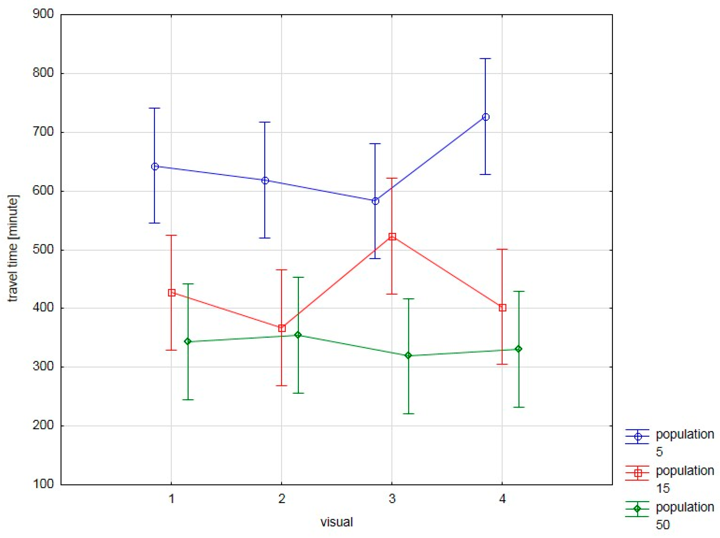
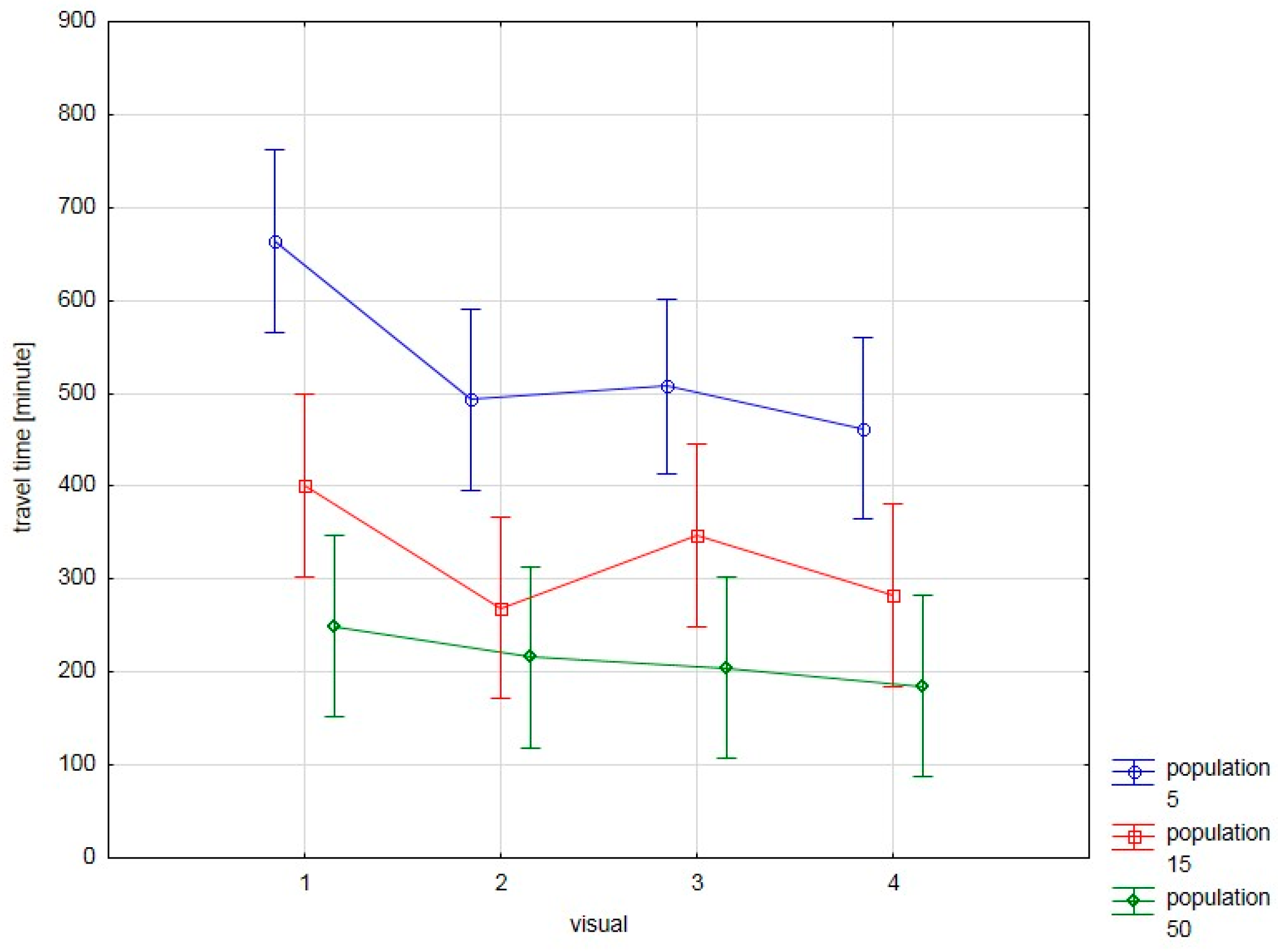
As we can see, the population size presents a strong effect (the travel time variable is explained by the population size variable in the proportion of more than 40%) in both cases; however, the visual either fails to indicate any influence (test instance 6/12) or shows a medium-size effect (test instance 6/48). The influence of the visual and population size parameters on the travel time obtained (vertical bars refer to 0.95 confidence intervals) are presented for both test instances in Figure 2 and Figure 3.
To investigate which of the parameters being tested, visual or population size, are different from each other, post hoc tests (Tukey tests) were conducted. Selected test results for test instance 6/48 are presented in Table 3. For the visual parameter, Tukey test showed essential differences of the average values between 1 and 2 and 4. In turn, for the population size parameter, tests showed essential differences between all the groups. For test instance 6/12, essential differences also occurred in all of the values of the population size parameter. Therefore, in our following tests, we assumed various sizes of population (5, 15, and 50) and visual = 3.
Each run of the CSO approach was terminated after 1000 iterations or if there was no improvement of the best solution through 25 iterations. In all tests: maxStep = 15, maxAttempt = 100. Table 4 shows the selected results of the CSO algorithm for the test instance with only one line, relating, however, to various sizes of population. For one line with 12 departures per day (marked as 1/12), the population consisting of 5 individuals is sufficient to find the best solution of travel time. Through 10 independent runs of the CSO approach, that solution was found in four cases. It turned out, however, that such a small number of solutions was not enough to solve the problem with 48 departures. The shortest travel time amounted to 1 h and 9 min. That value was obtained in three runs of the CSO algorithm. In the same test instance, the longest travel time amounted to 5 h and 21 min. Upon the increase of the population of individuals up to 15, we obtained the shortest travel time of 41 min in three runs. It is worth noting that the CSO algorithm, with the population of 50 solutions, generated the shortest travel time (41 min) in eight runs. What is interesting is that the worst solution for said population size was the same as the best solution for the population equal to 5.
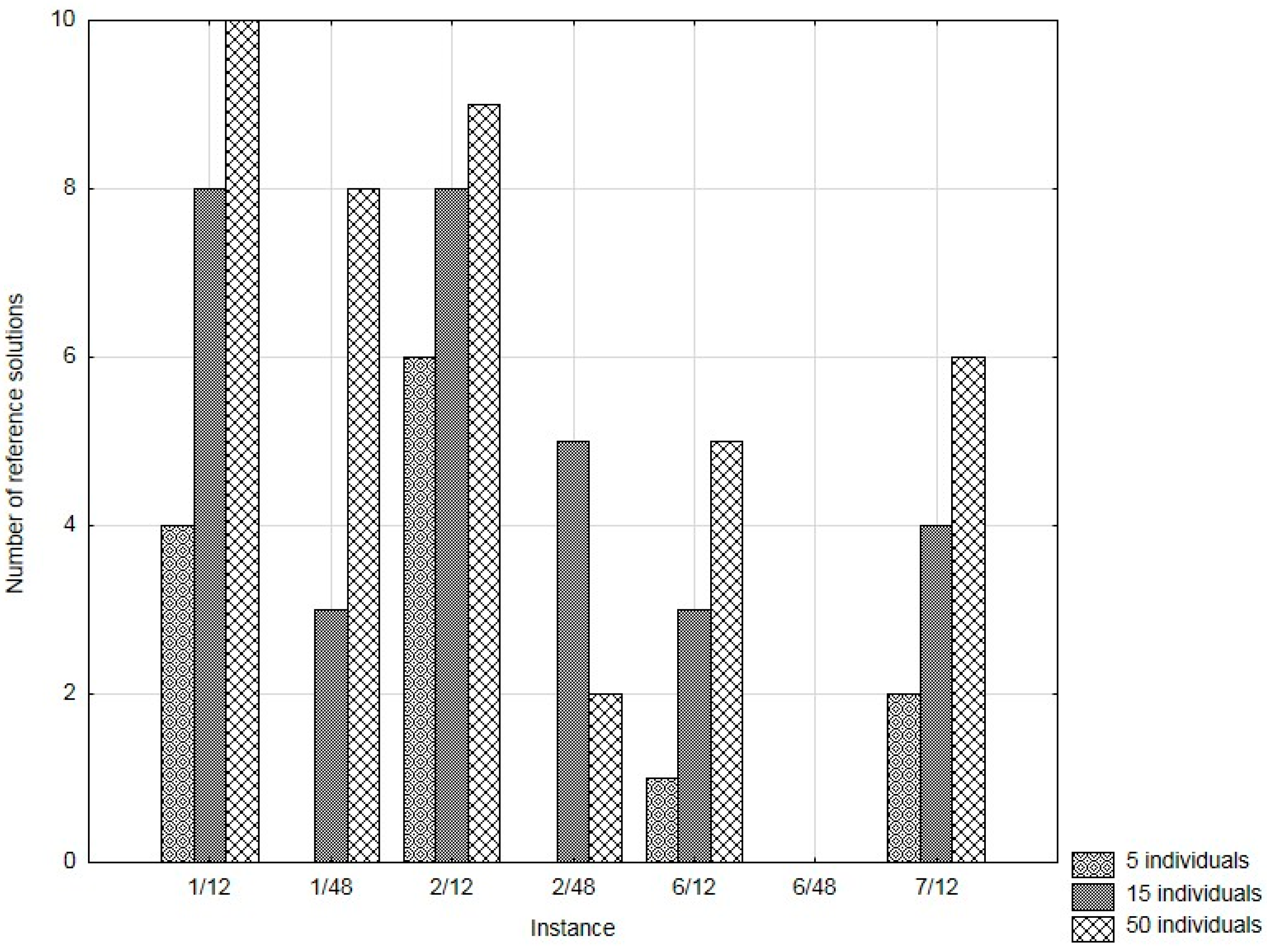
The number of correct solutions obtained during 10 runs, depending on the population size, is shown in Figure 4. As expected, the increased population improved the chance of finding the best solution. Note that in the test instance 6/48 (six lines and 48 departures per day), the best result could not be attained anyway.
For simpler TE models, relating to 12 departures a day, we obtained the best solution, although only in several runs.
However, with the population composed of five solutions, it was not possible to obtain the best known solution for any of the test instances in which 48 departures a day were taken into account (marked as 1/48, 2/48, and 6/48, respectively).
In addition, we implemented the particle swarm optimization algorithm. We assume that following the neighboring particles consist of attempts at “taking over” part of the graph edge from the solution of a better particle; that is, the particle that “follows” another one is trying to add to its route a node from the particle being followed. The number of nodes that is tried to be added is determined by the particle’s velocity. Moreover, we assumed that the difference of one hour in reaching the target node caused the increase of one node in the particle’s velocity.
Table 5 shows the experimental results of the CSO algorithm performance in comparison with the results obtained by Dijkstra’s and PSO algorithms for each test instance. Among the results obtained from the swarm algorithms, the best and the worst values of travel time were gathered. The first column shows the population size, the second one presents specific test instances, described by the numbers of lines and departures. The columns “Best travel” and “Worst travel” represent the best and worst travel times found by the CSO and the PSO algorithms, respectively. The fifth and the eighth columns give the average computational times of 10 independent runs of swarm algorithms. The last column shows reference solutions obtained by Dijkstra’s algorithm.
Depending on particular tests, and upon comparison with Dijkstra’s algorithm, the best results obtained with the CSO algorithm were similar to those of the second algorithm. In all of the test instances the results show that application of a larger population (50 individuals) reduced travel time, and produced the same solutions as Dijkstra’s algorithm in most cases. It needs to be pointed out that such an improvement was reached at the expense of computational time. Note that it does not imply that the optimum result was achieved. In the cases presented here, the result was not satisfying in one test instance with six lines and 48 departures per day.
When analyzing the results obtained with the use of the PSO algorithm, one can conclude that the CSO algorithm performs better than the PSO does. We should notice that the best travel times obtained with the PSO algorithm for two instances (6/12 and 6/48) are worse than those obtained with the use of the CSO algorithm. We should further consider the worst solutions, in all of the analyzed cases, there was a distinct domination of the CSO algorithm over the PSO one. Additionally, the average time of calculation performance, with the population increased to 50 individuals, indicates that the CSO algorithm provides a better solution when such specific parameters have been selected.

5. Conclusions

As we mentioned at the beginning of this work, we are merely presenting our research about the cockroach swarm optimization algorithm used to solve travel planning. Hence, we have shown that it is possible to use the CSO algorithm with the time-expanded model to solve travel planning, with some additional assumptions. To apply the CSO approach, we had to define movement in the search space. Therefore, we introduced a set of rules for determining paths in the time-expanded graph and some modifications of the searching capability during the whole algorithm. The proposed CSO approach was tested on seven instances of varying complexity. Solving travel planning was a complex process, but the results obtained were satisfactory. We compared the performance of the CSO, the PSO, and Dijkstra’s algorithms applied to the time-expanded model. Many experiments were conducted for different test problems and various sizes of population (5, 15, and 50). We also conducted some tests relating to the influence of visual and population size parameter settings on the results obtained, using the variance analysis (ANOVA). Our research proved that, in the majority of cases, the value of visual parameter did not have any significant influence on the travel time obtained. We observed that, for all the test instances, the increase of the population to up to 50 individuals improved the performance of the CSO algorithm, in respect of the travel time. However, it took more computational time, and it could be too slow to be used when solving larger problems. It should be mentioned, that for the test instance with six lines and 48 departures per day, the obtained solutions were not as good as those obtained with Dijkstra’s algorithm, but the improvement of travel time for the population of 50 individuals was clearly visible. However, our experiments indicated that the CSO method outperforms the PSO in terms of the best travel time.
Analyzing results, we observe that by introducing some modifications into the framework of the CSO approach, the approach can produce good solutions, but it requires the use of speed-up techniques or parallel computing. Therefore, one possibility for future research could examine the performance of a GPU implementation of our approach. Furthermore, the use of other models, instead of the time-expanded model, could lead to better results.

Acknowledgments

This paper was supported by the statutory research of AGH University of Science and Technology (no. 11.11.120.396).

Author Contributions

The concept of the CSO algorithm with the proposed modifications was designed by Joanna Kwiecień. The CSO approach, the PSO, and Dijkstra’s algorithms were implemented by Marek Pasieka. Material of Section 1, Section 2 and Section 3 was written by Joanna Kwiecień. The rest of the paper was written by both authors. All experiments were conceived, performed, and described by both authors. Authors have read and approved the final manuscript.

Conflicts of Interest

The authors declare no conflict of interest.

References

  1. Schulz, F.; Wagner, D.; Weihe, K. Dijkstra’s algorithm on-line: An empirical case study from public railroad transport. ACM J. Exp. Algorithmics 2000, 5, 1–23. [Google Scholar] [CrossRef]
  2. Schulz, F.; Wagner, D.; Zaroliagis, C. Using multi-level graphs for timetable information in railway systems. In Algorithm Engineering and Experiments; Mount, D.M., Stein, C., Eds.; Lecture Notes in Computer Science (LNCS); Springer: Heidelberg, Germany, 2002; Volume 2409, pp. 43–59. [Google Scholar]
  3. Pyrga, E.; Schulz, F.; Wagner, D.; Zaroliagis, C. Efficient Models for Timetable Information in Public Transportation Systems. ACM J. Exp. Algorithmics 2008, 12, 1–39. [Google Scholar] [CrossRef]
  4. Brodal, G.S.; Jacob, R. Time dependent networks as models to achieve fast exact time-table queries. Electron. Notes Theor. Comput. Sci. 2004, 92, 3–15. [Google Scholar] [CrossRef]
  5. Xing, B.; Gao, W. Innovative Computational Intelligence: A Rough Guide to 134 Clever Algorithms; Springer: Cham, Switzerland, 2014. [Google Scholar]
  6. Yang, X.-S. Nature-Inspired Metaheuristic Algorithms, 2nd ed.; Luniver Press: Frome, UK, 2010. [Google Scholar]
  7. Chen, Z. A modified cockroach swarm optimization. Energy Proced. 2011, 11, 4–9. [Google Scholar]
  8. Chen, Z.; Tang, H. Cockroach swarm optimization for vehicle routing problems. Energy Procedia 2011, 13, 30–35. [Google Scholar] [CrossRef]
  9. Cheng, L.; Wang, Z.; Yanhong, S.; Guo, A. Cockroach swarm optimization algorithm for TSP. Adv. Eng. Forum 2011, 1, 226–229. [Google Scholar] [CrossRef]
  10. Kwiecień, J.; Filipowicz, B. Comparison of firefly and cockroach algorithms in selected discrete and combinatorial problems. Bull. Pol. Acad. Sci. Tech. Sci. 2014, 62, 797–804. [Google Scholar] [CrossRef]
  11. Kwiecień, J. Use of different movement mechanisms in cockroach swarm optimization algorithm for traveling salesman problem. In Artificial Intelligence and Soft Computing; Rutkowski, L., Korytkowski, M., Scherer, R., Tadeusiewicz, R., Zadeh, L.A., Zurada, J.M., Eds.; Lecture Notes in Computer Science (LNCS); Springer: Cham, Switzerland, 2016; Volume 9693, pp. 484–493. [Google Scholar]
  12. Obagbuwa, I.C.; Abidoye, A.P. Binary cockroach swarm optimization for combinatorial optimization problem. Algorithms 2016, 9, 59. [Google Scholar] [CrossRef]
  13. Bast, H.; Delling, D.; Goldberg, A.; Müller-Hannemann, M.; Pajor, T.; Sanders, P.; Wagner, D.; Werneck, R.F. Route Planning in Transportation Networks. In Algorithm Engineering; Kliemann, L., Sanders, P., Eds.; Lecture Notes in Computer Science (LNCS); Springer: Cham, Switzerland, 2016; Volume 9220, pp. 19–80. [Google Scholar]
  14. Müller-Hannemann, M.; Schulz, F.; Wagner, D.; Zaroliagis, C. Timetable information: Models and algorithms. In Algorithmic Methods for Railway Optimization; Geraets, F., Kroon, L.G., Schoebel, A., Wagner, D., Zaroliagis, C.D., Eds.; Lecture Notes in Computer Science (LNCS); Springer: Heidelberg, Germany, 2007; Volume 4359, pp. 67–90. [Google Scholar]
  15. Mohemmed, A.W.; Sahoo, N.C.; Geok, T.K. Solving shortest path problem using particle swarm optimization. Appl. Soft Comput. 2008, 8, 1643–1653. [Google Scholar] [CrossRef]
  16. Zhang, Y.; Jun, Y.; Wei, G.; Wu, L. Find multi-objective paths in stochastic networks via chaotic immune PSO. Expert Syst. Appl. 2010, 37, 1911–1919. [Google Scholar] [CrossRef]
  17. Effati, S.; Jafarzadeh, M. Nonlinear neural networks for solving the shortest path problem. Appl. Math. Comput. 2007, 189, 567–574. [Google Scholar] [CrossRef]
  18. Zhang, Y.; Wu, L.; Wei, G.; Wang, S. A novel algorithm for all pairs shortest path problem based on matrix multiplication and pulse coupled neural network. Digit. Signal Process. 2011, 21, 517–521. [Google Scholar] [CrossRef]
  19. Rajabi-Bahaabadi, M.; Shariat-Mohaymany, A.; Babaei, M.; Ahn, C.W. Multi-objective path finding in stochastic time-dependent road networks using non-dominated sorting genetic algorithm. Expert Syst. Appl. 2015, 42, 5056–5064. [Google Scholar] [CrossRef]
  20. Wang, S.; Yang, J.; Liu, G.; Du, S.; Yan, J. Multi-objective path finding in stochastic networks using a biogeography-based optimization method. Simulation 2016, 92, 637–647. [Google Scholar] [CrossRef]
  21. Gen, M.; Cheng, R.; Wang, D. Genetic algorithms for solving shortest path problems. In Proceedings of the 1997 IEEE International Conference on Evolutionary Computing, Indianapolis, IN, USA, 13–16 April 1997; pp. 401–406. [Google Scholar]
  22. Davies, C.; Lingras, P. Genetic algorithms for rerouting shortest paths in dynamic and stochastic networks. Eur. J. Oper. Res. 2003, 144, 27–38. [Google Scholar] [CrossRef]
  23. Lozano, A.; Storchi, G. Shortest viable path algorithm in multimodal networks. Transp. Res. Part A Policy Pract. 2001, 35, 225–241. [Google Scholar] [CrossRef]
  24. Ma, T.Y. An A label-setting algorithm for multimodal resource constrained shortest path problem. Procedia Soc. Behav. Sci. 2014, 111, 330–339. [Google Scholar] [CrossRef]
  25. Zhang, Y.; Liu, P.; Yang, L.; Gao, Y. A bi-objective model for uncertain multi-modal shortest path problems. J. Uncertain. Anal. Appl. 2015, 3, 8. [Google Scholar] [CrossRef]
  26. Horn, M.E.T. An extended model and procedural framework for planning multi-modal passenger journeys. Transp. Res. Part B Methodol. 2003, 37, 641–660. [Google Scholar] [CrossRef]
  27. Liu, L.; Yang, J.; Mu, H.; Li, X.; Wu, F. Exact algorithm for multi-criteria multi-modal shortest path with transfer delaying and arriving time-window in urban transit network. Appl. Math. Model. 2014, 38, 2613–2629. [Google Scholar] [CrossRef]
  28. Yu, H.; Lu, F. A multi-modal route planning approach with an improved genetic algorithm. Adv. Geo-Spat. Inform. Sci. 2012, 38, 193–202. [Google Scholar]
  29. Dijkstra, E.W. A note on two problems in connexion with graphs. Numer. Math. 1959, 1, 269–271. [Google Scholar] [CrossRef]
  30. Fu, L.; Sun, D.; Rilett, L.R. Heuristic shortest path algorithms for transportation applications: State of the art. Comput. Oper. Res. 2006, 33, 3324–3343. [Google Scholar] [CrossRef]
  31. Dib, O.; Manier, M.-A.; Caminada, A. Memetic algorithm for computing shortest paths in multimodal transportation networks. Transp. Res. Procedia 2015, 10, 745–755. [Google Scholar] [CrossRef]
  32. Dibbelt, J.; Pajor, T.; Strasser, B.; Wagner, D. Intriguingly simple and fast transit routing. In Experimental Algorithms; Bonifaci, V., Demetrescu, C., Marchetti-Spaccamela, A., Eds.; Lecture Notes in Computer Science (LNCS); Springer: Heidelberg, Germany, 2013; Volume 7933, pp. 43–54. [Google Scholar]
  33. Delling, D.; Pajor, T.; Werneck, R.F. Round-based public transit routing. Transp. Sci. 2015, 49, 591–604. [Google Scholar] [CrossRef]
  34. Delling, D.; Dibbelt, J.; Pajor, T.; Wagner, D.; Werneck, R.F. Computing Multimodal Journeys in Practice. In Experimental Algorithms; Bonifaci, V., Demetrescu, C., Marchetti-Spaccamela, A., Eds.; Lecture Notes in Computer Science (LNCS); Springer: Heidelberg, Germany, 2013; Volume 7933, pp. 260–271. [Google Scholar]
  35. Bast, H.; Storandt, S. Frequency-based search for public transit. In Proceedings of the 22nd ACM SIGSPATIAL International Conference on Advances in Geographic Information Systems, Dallas, TX, USA, 4–7 November 2014; pp. 13–22. [Google Scholar]
  36. Delling, D.; Pajor, T.; Wagner, D. Engineering time-expanded graphs for faster timetable information. In Robust and Online Large-Scale Optimization; Ahuja, R.K., Möhring, R.H., Zaroliagis, C.D., Eds.; Lecture Notes in Computer Science (LNCS); Springer: Heidelberg, Germany, 2009; Volume 5868, pp. 182–206. [Google Scholar]
  37. Geisberger, R. Advanced Route Planning in Transportation Networks. Ph.D. Thesis, Karlsruhe Institute of Technology, Baden-Württemberg, Germany, February 2011. [Google Scholar]
  38. Poli, R.; Kennedy, J.; Blackwell, T. Particle swarm optimization. An overview. Swarm Intell. 2007, 1, 33–57. [Google Scholar] [CrossRef]
  39. Toofani, A. Solving routing problem using particle swarm optimization. Int. J. Comput. Appl. 2012, 52, 16–18. [Google Scholar] [CrossRef]
Figure 1. Rules to create the initial population.
Entropy 19 00213 g001
Figure 2. The influence of the selected parameters (test instance 6/12).
Entropy 19 00213 g002
Figure 3. The influence of the selected parameters (test instance 6/48).
Entropy 19 00213 g003
Figure 4. Number of the best solutions depending on the population size.
Entropy 19 00213 g004
Table 1. Characteristics of the time-expanded model.
Number of Lines Number of StopsDaily Number of DeparturesNumber of Arrival NodesNumber of Departure NodesNumber of Transfer NodesTotal Number of Nodes
12112217229228674
121488659139122690
233123613853841130
233481441153715364514
652126737457442162
652482689297729768642
752126747477462167
Table 2. Results of the ANOVA test for instances 6/12 and 6/48.
InstanceEffectpη2
6/12visual0.790.01
population size00.43
visual × population size 0.170.07
6/48visual0.010.1
population size00.44
visual × population size0.740.03
Table 3. Results of Tukey test (test instance 6/48).
Visual{1}{2}{3}{4}
1 0.0324970.1960310.010639
20.032497 0.8531300.979342
30.1960310.853130 0.628842
40.0106390.9793420.628842
Table 4. Results for one line.
PopulationDaily Number of DeparturesTravel Time [h:min]Computational Time [ms]
51200:45, 00:45, 02:45, 00:45, 02:45, 02:45, 02:45, 02:45, 06:45, 00:4538, 23, 9, 10, 6, 10, 5, 4, 8, 3
151200:45, 00:45, 00:45, 00:45, 02:45, 00:45, 00:45, 02:45, 00:45, 00:45108, 56, 13, 31, 16, 9, 18, 8, 7, 9
501200:45, 00:45, 00:45, 00:45, 00:45, 00:45, 00:45, 00:45, 00:45, 00:45,110, 82, 52, 56, 31, 50, 43, 64, 50, 35
54803:29, 02:05, 05:21, 03:01, 05:21, 01:09, 03:01, 03:57, 01:09, 01:09 17, 11, 6, 4, 2, 4, 2, 3, 3, 2
154800:41, 00:41, 01:37, 03:01, 01:37, 00:41, 04:25, 01:09, 01:09, 01:3758, 15, 10, 12, 12, 11, 14, 11, 6, 12
504800:41, 00:41, 00:41, 00:41, 00:41, 01:09, 00:41, 00:41, 01:09, 00:4128, 29, 33, 94, 29, 30, 46, 43, 26, 47
Table 5. Selected results of seven test instances.
PopulationInstanceCSOPSODijkstra [h:min]
Best Travel [h:min]Worst Travel [h:min]Mean Time [ms]Best Travel [h:min]Worst Travel [h:min]Mean Time [ms]
51/1200:4506:4511.600:4508:4511:500:45
151/1200:4502:4527.500:4502:4530.8
501/1200:4500:4557.300:4500:45172.8
51/4801:0905:215.400:4111:532.700:41
151/4800:4104:2516.100:4105:2116.3
501/4800:4101:0940.500:4101:3790.0
52/1202:3808:384.202:3816:385.602:38
152/1202:3804:3833.802:3812:3825.2
502/1202:3804:3884.102:3804:38215.3
52/4802:3109:4316.302:3113:433.501:07
152/4801:0703:5528.301:0711:2316.5
502/4801:0702:03131.601:0708:35187
56/1204:0718:0714.814:0722:079.304:07
156/1204:0712:0731.708:0714:0774.5
506/1204:0706:07122.306:0710:07272.3
56/4803:2211:4611.611:1817:223.801:02
156/4801:5808:3042.105:4213.3836
506/4801:3005:42187.502:5413:38301.1
57/1204:0712:0715.108:0716:071204:07
157/1204:078:0738.504:0716:0756.3
507/1204:076:07153.104:0708:07284

