Fourier’s Law in a Generalized Piston Model

Abstract

A simplified, but non trivial, mechanical model—gas of N particles of mass m in a box partitioned by n mobile adiabatic walls of mass M—interacting with two thermal baths at different temperatures, is discussed in the framework of kinetic theory. Following an approach due to Smoluchowski, from an analysis of the collisions particles/walls, we derive the values of the main thermodynamic quantities for the stationary non-equilibrium states. The results are compared with extensive numerical simulations; in the limit of large n, $mN/M\gg 1$ and $m/M\ll 1$, we find a good approximation of Fourier’s law.

1. Introduction

Fourier’s law, which relates the macroscopic heat flux to the temperature gradient in a solid system, was introduced almost two centuries ago. Nevertheless, its understanding from microscopic basis is still an important open issue of the non-equilibrium statistical mechanics [1]. In particular, among the several theoretical studies on this subject, important results have been derived mainly for $1d$ systems. The prototype model is a chain of masses and non linear springs (Fermi-Pasta-Ulam-like systems), whose ends interacts with thermal baths at different temperatures [1,2,3]. Other investigated systems are constituted of $1d$ lattices [4,5], chains of cells, with an energy storage device, which exchange energy through tracer particles [6,7], spinning disks [8], systems with local thermalization mechanism [9,10], or a chain of anharmonic oscillators with local energy conserving noise [11]. Despite the apparent simplicity of the problem, and of the considered models, both the analytical approaches and the numerical studies are rather difficult in this context.

The main aim of the present paper is the study of Fourier’s law using a mechanical model, which is rather crude (but still non-trivial), allowing for an approach in terms of kinetic theory. More specifically, we consider a generalized piston model, made of a certain number of cells, each containing a non-interacting particle gas. The walls of the cells are mobile, massive objects, that interact with the particles via elastic collisions. The system at its ends interacts with thermal baths at fixed temperatures. It is easy to realize the analogy between such a generalized piston model and the systems of masses and springs: the pistons and the gas compartments play the role of masses and springs, respectively.

Our model is an example of partitioning system (as the adiabatic piston), where previous studies showed that the presence of mobile walls can induce interesting behaviours [12,13,14,15,16,17,18,19,20,21]. Basically, in the study of partitioning systems, one can adopt two approaches: in terms of a Boltzmann equation [14] or introducing effective equations (Langevin-like) for suitable observables derived à la Smoluchowski, i.e., from an analysis of the collisions particles/walls. In our study, we will adopt the latter method.

The paper is organized as follows. Section 1 is devoted to the introduction of the model; in Section 2, we show how a thermodynamic approach is not sufficient to determine the values of macroscopic variables in the steady state. In Section 3, we present a coarse-grained Smoluchowski-like description of the system, which provides a good prediction for the main quantities of interest. In Section 4, we compare the theoretical results with numerical simulations and discuss the limit of validity of the proposed approach. In Section 5, some general conclusions on Fourier’s Law in mechanical systems are drawn. In Appendix A, we report the details of the analytical computations presented in Section 3.

2. A Generalized Piston Model

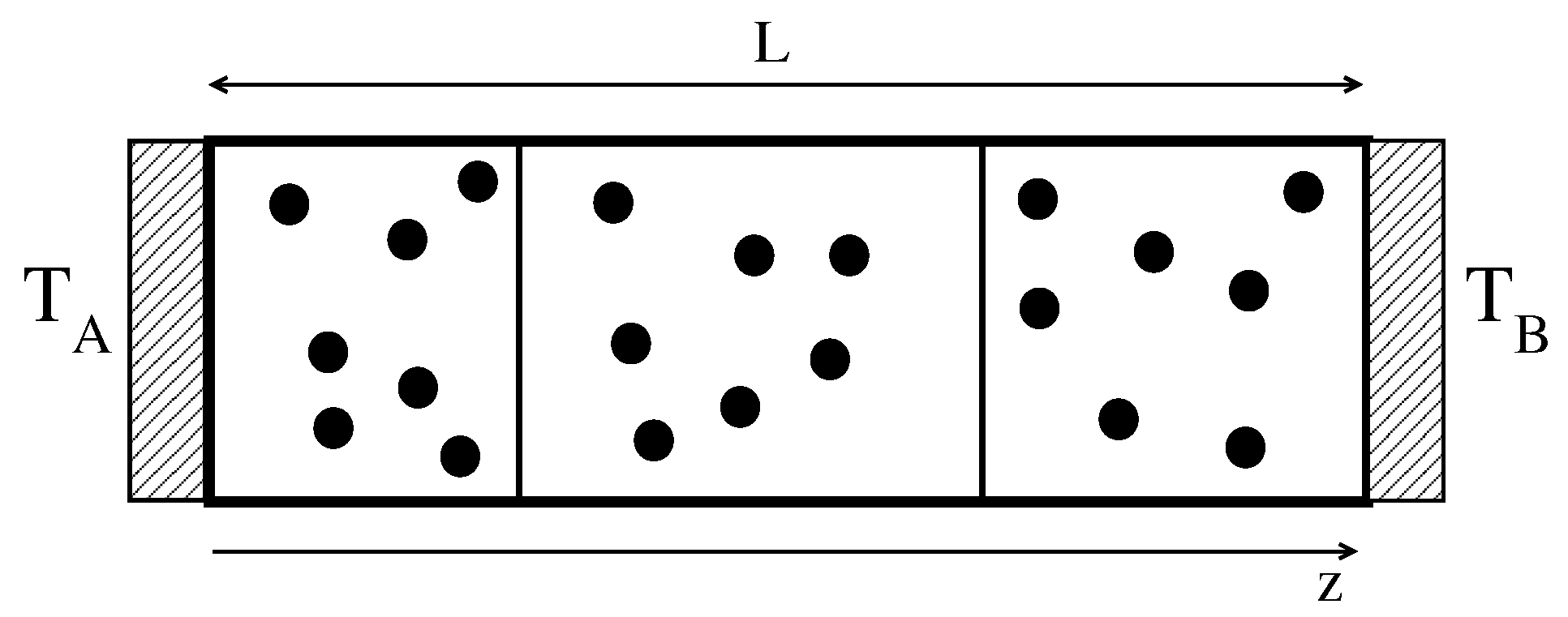
We consider a box of length L, partitioned by n mobile adiabatic walls (also called pistons in the following), with mass M, average positions $z_j$ and velocities $V_j$ ($j=1,2,\cdots n$). The walls move without friction along the horizontal axis (see Figure 1). The external walls are kept fixed in the positions $z_0=0$ and $z_{n+1}=L$. Each of the $n+1$ compartments separated by the walls contains N non-interacting point-like particles, with mass m, positions $x_i$ and velocities $v_i$. The particles interact with the pistons via elastic collisions:

$$\begin{array}{cc}\hfill V^{\prime }& =V+\frac{2m}{m+M}(v_i-V),\hfill \\ \hfill v_i^{\prime }& =v_i-\frac{2M}{m+M}(v_i-V),\hfill \end{array}$$

(1)

where primes denote post-collisional velocities.

The two external walls in $z=0$ and $z=L$ act as thermal baths at temperatures $T_A$ and $T_B$. The interaction of the thermostats with the particles is the following: when a particle collides with the wall, it is reinjected into the system with a new velocity drawn from the probability distribution [22]

$${\rho }_{A,B}\left(v^{\prime }\right)=\frac{m}{k_B{T}_{A,B}}\left|v^{\prime }\right|e^{-\frac{m{v}^{\prime 2}}{2k_B{T}_{A,B}}}\mathsf{\Theta }(\pm v^{\prime }),$$

(2)

with + for the case A and − for B, and $k_B$ is the Boltzmann constant, $\mathsf{\Theta }\left(x\right)$ being the Heaviside step function:

$$\mathsf{\Theta }\left(x\right)=\left\{\begin{array}{cc}1,\hfill & \mathrm{if}x>0,\hfill \\ 0,\hfill & \mathrm{if}x\le 0.\hfill \end{array}\right.$$

(3)

For the following discussion, we define the temperature of the $i-$th piston as

$$T_i^{\left(p\right)}=M\langle V_i^2\rangle ,$$

(4)

and the temperature of the particle gas in the compartment j as an average on the particles between the $(j-1)$-th and the j-th piston

$$T_j=m\frac{1}{N}\sum _{i\in (j-1)N}^{jN}\langle v_i^2\rangle .$$

(5)

3. Simple Thermodynamic Considerations

We expect, and this is fully in agreement with the numerical computations, that, given a generic initial condition, after a certain transient, the system reaches a stationary state. The positions of the walls fluctuate around their mean values $z_j$, in a similar way to $T_i^{\left(p\right)}$ and $T_i$. The first non-trivial problem of the non equilibrium statistical mechanics is to determine $z_j$, $T_i^{\left(p\right)}$ and $T_i$ as function of the parameters of the model, i.e., $n,L,m,M,T_A$ and $T_B$.

We first analyze the simplest case of a single piston, where thermodynamics is sufficient to provide a complete description of the stationary state. Then, we consider the more general case of a multiple piston; in such a situation, thermodynamic relations are not enough to univocally determine the steady state: it is necessary to adopt a statistical mechanics approach. Such an approach will rely on three main assumptions, discussed in more detail below: small mass ratio $m/M\ll 1$, local thermodynamic equilibrium in each compartment, and independence of the collisions particles/pistons.

3.1. Single Piston

If $n=1$, using the equation for the perfect gas in each compartment, we immediately get the equations

$$\left\{\begin{array}{c}p{z}_1=N{k}_B{T}_A,\hfill \\ p(L-z_1)=N{k}_B{T}_B,\hfill \end{array}\right.$$

(6)

where p is the pressure, yielding

$$z_1=\frac{T_A}{T_A+T_B}L.$$

(7)

Therefore, in this case, thermodynamics univocally determines the stationary state of the system.

3.2. Multiple Piston

We now consider the generalized piston model with $n>1$. An analysis of the case $n=2$ is enough to understand how the relations obtained from thermodynamics can be not sufficient to fully characterize the non equilibrium steady state. Indeed, we have the following relations:

$$\left\{\begin{array}{c}p{z}_1=N{k}_B{T}_A,\hfill \\ p(z_2-z_1)=N{k}_B{T}_1,\hfill \\ p(L-z_2)=N{k}_B{T}_B,\hfill \end{array}\right.$$

(8)

which give the constraints

$$\begin{array}{c}\hfill z_1=\frac{T_A}{T_A+T_1+T_B}L,\\ \hfill z_2=\frac{T_A+T_1}{T_A+T_1+T_B}L.\end{array}$$

(9)

Therefore, since we have three variables ($z_1,z_2,T_1$) and only two constraints, thermodynamics is not enough to determine the stationary state. The computation can be easily extended to an arbitrary value of n, leading to

$$\left\{\begin{array}{c}p{z}_1=N{k}_B{T}_A,\hfill \\ p(z_2-z_1)=N{k}_B{T}_1\hfill \\ ...,\hfill \\ p(z_n-z_{n-1})=N{k}_B{T}_{n-1},\hfill \\ p(L-z_n)=N{k}_B{T}_B,\hfill \end{array}\right.$$

(10)

that give the conditions

$$\begin{array}{c}{z}_1=\frac{T_A}{T_A+{\sum }_{k=1}^{n-1}{T}_k+T_B}L,\cdots z_m=\frac{T_A+{\sum }_{k=1}^{m-1}{T}_k}{T_A+{\sum }_{k=1}^{n-1}{T}_k+T_B}L,\cdots z_n=\frac{T_A+{\sum }_{k=1}^{n-1}{T}_k}{T_A+{\sum }_{k=1}^{n-1}{T}_k+T_B}L,\hfill \end{array}$$

(11)

with $m=2,\dots ,n-1$, namely, only n constraints for $2n-1$ variables.

4. Coarse-Grained Description and Effective Langevin Equations

In order to obtain a statistical description of the system, we now derive effective stochastic equations, governing the dynamics of the relevant variables. Previous theoretical studies based on a Boltzmann equation approach on similar systems were reported in [13,14,15]. In particular, a generalized piston model was considered in Reference [15]. In those works, theoretical results were not compared to numerical simulations, so that the underlying hypotheses and their range of validity remained unclear.

Here, we present a different analysis. We will assume that the evolution of the observables is described by Langevin equations. The idea, coming back to Smoluchowski, is to integrate out the fast degrees of freedom of the gas particles by computing conditional averages, knowing the macroscopic variables: position z and velocity V of each piston, and temperatures T of the gases. In order to simplify the notation, let us denote by $〈·〉$ this average, meaning the conditional average $〈·|z,V,T〉$. We will compute the average change of a generic observable X in a small time interval $\Delta t$, due to the collisions between the particles of the gas and the pistons.

Let us assume that in the stationary state the particles of the gas, in each compartment, have uniform space distribution $\rho$ and a Maxwell–Boltzmann distribution $\varphi \left(v\right)$ at temperature T:

$$\varphi \left(v\right)=\sqrt{\frac{m}{2\pi k_{B}T}}{e}^{-\frac{m}{2k_{B}T}{v}^2},\rho \left(x\right)=\frac{1}{\Delta z},$$

(12)

where $\Delta z$ is the length of the box containing the gas. We can obtain the rate of the collisions by considering the following equivalent problem: piston at rest and a particle, which moves with the relative velocity $v-V$. The point particles which collide against the piston in x in the time interval $dt$ are:

$$N\rho \left(x\right)(v-V)\mathsf{\Theta }(v-V)dt,N\rho \left(x\right)(V-v)\mathsf{\Theta }(V-v)dt,$$

(13)

respectively, for particles on the left and on the right with respect to the piston. The Heaviside function $\mathsf{\Theta }$ is necessary to have a collision.

Let us now consider a generic observable $X_j$, depending in general on the velocities of the gas particles and of the pistons. We want to write down a Langevin equation:

$$\frac{d{X}_j}{dt}=D_j\left(\mathbf{X}\right)+\mathrm{noise},$$

(14)

where both the drift term $D_j\left(\mathbf{X}\right)$ ($\mathbf{X}$ being the vector of all relevant macroscopic variables in the system) and the noise term are due to collisions with the particles of the gas. We have:

$$D_j\left(\mathbf{X}\right)=\underset{\Delta t\to 0}{lim}\frac{〈\Delta X_j|\mathbf{X}〉}{\Delta t}=\underset{\Delta t\to 0}{lim}\frac{1}{\Delta t}\left[{〈\Delta X_j〉}_{coll}^L+{〈\Delta X_j〉}_{coll}^R\right],$$

(15)

where

$$\begin{array}{cc}\hfill {〈\Delta X_j〉}_{coll}^R& =N{\int }_V^{\infty }dv{\int }_{z_L-(v-V)\Delta t}^{z_L}dx{X}_j\rho \left(x\right)\varphi \left(v\right)\mathsf{\Theta }(v-V)=\frac{N}{\Delta z_L}{\int }_V^{\infty }dv{X}_j\varphi \left(v\right)(v-V)\Delta t,\hfill \end{array}$$

(16)

$$\begin{array}{cc}\hfill {〈\Delta X_j〉}_{coll}^L& =N{\int }_{-\infty }^{V}dv{\int }_{z_R}^{z_R-(v-V)\Delta t}dx{X}_j\rho \left(x\right)\varphi \left(v\right)\mathsf{\Theta }(V-v)=\frac{N}{\Delta z_R}{\int }_{-\infty }^{V}dv{X}_j\varphi \left(v\right)(V-v)\Delta t.\hfill \end{array}$$

(17)

${〈\Delta X_j〉}_{coll}^R$ is the variation of the observable due to the collisions with the particles that have the pistons on the left, while ${〈\Delta X_j〉}_{coll}^L$ denotes the variation due to the collisions with the particles which have the piston on the right.

In the stationary state, the macroscopic variables T, V and z do not depend on time. It means that the time derivative of the conditional average of a generic observable X is zero, namely:

$$\underset{\Delta t\to 0}{lim}\frac{1}{\Delta t}\left[{〈\Delta X_j〉}_{coll}^L+{〈\Delta X_j〉}_{coll}^R\right]=0.$$

(18)

By using a perturbation development in the small parameter $ϵ=m/M$, it is possible to derive the relations between the average positions and the temperatures of the pistons and the temperatures of the gas. In order to obtain this result, we need to average on the piston velocity, which is a stochastic variable. Of course, in the steady state, the odd momenta have to be zero:

$$〈V^{2\alpha +1}〉=0,\alpha =0,1,2,...$$

(19)

The idea is to compute the average force produced by the particles of the gas, which collide against the piston, by computing the average momentum exchanged in the collisions.

The evolution of the velocity of the piston is governed by the following stochastic differential equation:

$$M\frac{d}{dt}V=F_{coll}(\Delta z_L,\Delta z_R,T_L,T_R,V)+K\eta ,$$

(20)

where $\eta$ is zero-average white noise, usually K is a constant, and $F_{coll}$ is the average force which acts on the piston. This force is due to the collisions with the gas on the left and on the right, and depends on the average size of the box on the right and on the left of the piston, $\Delta z_L$ and $\Delta z_R$, respectively, and on the temperatures of the gas on the left and on the right, $T_L$ and $T_R$. Now let us set $\Delta X=V^{\prime }-V$ in Equation (15). As detailed in the Appendix A, computing the left and right contributions to $F_{coll}$ and expanding in the small mass ratio $ϵ=\sqrt{m/M}$, we obtain at the lowest orders:

$$O\left(1\right):N{k}_B\left(\frac{T_L}{\Delta z_L}-\frac{T_R}{\Delta z_R}\right),$$

(21)

$$O\left(ϵ\right):-2N\sqrt{2k_B}\sqrt{\frac{M}{\pi }}\left[\frac{T_L^{1/2}}{\Delta z_L}+\frac{T_R^{1/2}}{\Delta z_R}\right]V.$$

(22)

In the steady state, when the time derivative vanishes, we have from the order $O\left(1\right)$ the following relation between the temperatures of the gas and the average length of the boxes:

$$\Delta z_R=\Delta z_L\frac{T_R}{T_L}.$$

(23)

This relation is nothing but the one that can be derived from thermodynamics. From Equation (22), we obtain the obvious result $\langle V\rangle =0$.

Analogous computations, reported in the Appendix A, can be carried out for the variance of the pistons and the gas temperatures. In particular, for the variable $\Delta X=M(V^{\prime 2}-V^2)$, at lowest orders in $ϵ$, we obtain the relations:

$$O\left(1\right):N2k_B\left(\frac{T_L}{\Delta z_L}-\frac{T_R}{\Delta z_R}\right),$$

(24)

$$O\left(ϵ\right):\frac{N}{\sqrt{\pi }}\frac{4\sqrt{2}}{M^{1/2}}\left[\left(\frac{{\left(k_B{T}_L\right)}^{3/2}}{\Delta z_L}+\frac{{\left(k_{B}T\right)}^{3/2}}{\Delta z_R}\right)-M{V}^2\left(\frac{{\left(k_B{T}_R\right)}^{1/2}}{\Delta z_R}+\frac{{\left(k_B{T}_L\right)}^{1/2}}{\Delta z_L}\right)\right].$$

(25)

In the steady state, by using the thermodynamic relations, the order $O\left(1\right)$ Equation (24) is identically zero. After integrating over all values of the piston velocity and by requiring that the order $O\left(ϵ\right)$ vanishes, we obtain a relation between the temperature of the piston $T^{\left(p\right)}$ and those of the gases on the left and on the right:

$$T^{\left(p\right)}=M〈V^2〉={\left(T_R{T}_L\right)}^{1/2}.$$

(26)

Finally, a condition on the temperature of the gas as a function of the velocity variance of the pistons on its left and on its right can be obtained by considering the variable $\Delta X=m(v^{\prime 2}-v^2)/N$ in Equation (15). This gives (see Appendix A) the relations:

$$O\left(1\right):\frac{2k_{B}T}{\Delta z}\left(V_L-V_R\right),$$

(27)

$$O\left(ϵ\right):\frac{\sqrt{2k_B}}{\Delta z}\frac{4}{\sqrt{\pi }}\frac{T^{1/2}}{M^{1/2}}\left[M{V}_R^2+M{V}_L^2-2T\right].$$

(28)

By integrating over the velocity of the piston, because $〈V〉$ is zero, the order $O\left(1\right)$ is identically zero. By requiring that, in the stationary state, the order $O\left(ϵ\right)$ vanishes, we eventually obtain:

$$\begin{array}{c}0=\frac{\sqrt{2k_B}}{\Delta z}\frac{4}{\sqrt{\pi }}\frac{T^{1/2}}{M^{1/2}}\left[M{〈V_R^2〉}_0+M{〈V_L^2〉}_0-2T\right]⟹T=\frac{M}{2}\left(〈V_R^2〉+〈V_L^2〉\right).\hfill \end{array}$$

(29)

As expected from thermodynamics, one can easily show that the gases in contact with the thermostats reach the temperatures of the thermal baths (see Appendix A for a detailed explanation).

5. Numerical Simulations

In order to check the range of validity of the above approach, we have performed extensive molecular dynamics simulations (using an event driven algorithm) of the system, varying the relevant parameters of the model and comparing the analytical prediction of Section 3 with the actual numerical results. The system is initialized with the pistons placed at equidistant positions, with zero velocity, while the gas particles are randomly distributed in each box, with velocities drawn from a Gaussian distribution at temperature intermediate with respect to those of the thermostats. We have, however, checked that the stationary state reached by the system is independent of the initial conditions. All data presented in the following are measured in the steady state, after the transient relaxation dynamics from the initial state.

In Figure 2, we show the piston temperatures $T_i^{\left(p\right)}$, $i=1,2,3$, for a 3-piston system, as measured in numerical simulations (symbols) for a certain choice of the parameters, and compare them with the theoretical predictions of Equation (26) (lines). The approximation is good for the intermediate piston, while it is not very accurate for the side pistons, and is the worst in the case of a large gradient $T_B/T_A\gg 1$. Simulations performed for systems with more pistons give similar results.

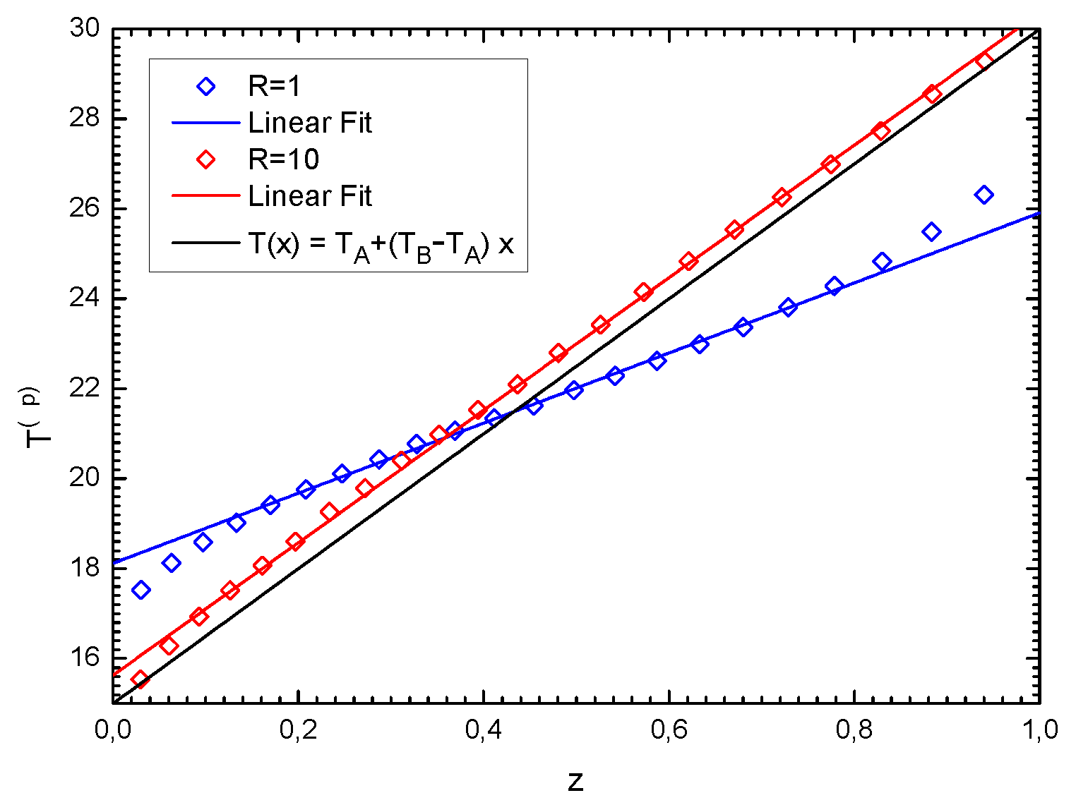
In Figure 3, we consider a system with a large number of pistons (n = 22), where the temperature profile shows a linear behavior, in agreement with Fourier’s law. We report two sets of data, differing in the value of the parameter $R=mN/M$. Notice that the linear behavior extends for a wider range of z in the case $R=10$. Lines represent linear fits of the data. Let us note that, for large n and $R\gg 1$, $T^{\left(p\right)}$ vs. z is in good agreement with a linear behavior in the whole space interval (even close to the thermal baths).

The derivation of the Langevin equation (see Appendix A) is mainly based on the assumptions:

• $m/M\ll 1$;
• a local thermodynamic equilibrium, i.e. in each compartment between the piston $i-1$ and the piston i, the spatial distribution of the particles is uniform and the velocity probability distribution is a Gaussian function, whose variance is given by the gas temperature;
• the collisions particles/pistons are independent.

The first assumption is easily checked, while the other ones are more difficult. We can expect that a necessary condition for their validity is that N must be large. We have measured the velocity distribution of the gas particles in the numerical simulations, finding that the above hypothesis is verified. Moreover, we expect that the number of recollisions decreases with the ratio $m/M$, and we have numerically checked that their contribution is negligible (the fraction of recollisions on the total number of collisions is about $0.1\%$). 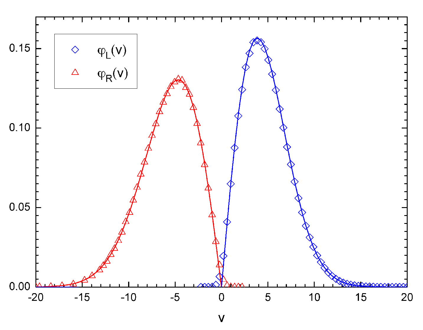Figure 4 shows the probability distribution functions of particles colliding from left, ${\varphi }_L\left(v\right)$, and from right, ${\varphi }_R\left(v\right)$, with a moving wall: the agreement with a Gaussian assumption is rather evident.

In addition, the numerical computations show that the left- and right-moving particles in the same compartment have the following probability distributions:

$$\begin{array}{ccc}\hfill {\varphi }_{-}\left(v\right)& =& \sqrt{\frac{2m}{\pi k_B{T}_{-}}}\mathsf{\Theta }\left(v\right)e^{-\frac{m{v}^2}{2k_B{T}_{-}}},\hfill \end{array}$$

(30)

$$\begin{array}{ccc}\hfill {\varphi }_{+}\left(v\right)& =& \sqrt{\frac{2m}{\pi k_B{T}_{+}}}\mathsf{\Theta }(-v)e^{-\frac{m{v}^2}{2k_B{T}_{+}}},\hfill \end{array}$$

(31)

where $T_{-}$ ($T_{+}$) denotes the temperature of the particles incident on the piston i ($i-1$) from the left (right), with $T_{-}\approx T_{+}$, resulting in a small but finite heat flow proportional to $(T_{-}-T_{+})$, in agreement with [15]. Let us note that the above probability distributions are different from the distributions ${\varphi }_L\left(v\right)$ and ${\varphi }_R\left(v\right)$, which are computed for particles actually colliding with the piston; this is the origin of the presence of the factor v appearing in the expressions in the caption of Figure 4.

The distribution of v in the compartment between pistons $i-1$ and i, has the form:

$$\varphi \left(v\right)\propto A\mathsf{\Theta }\left(v\right)e^{-\frac{m{v}^2}{2k_B{T}_{-}}}+B\mathsf{\Theta }(-v)e^{-\frac{m{v}^2}{2k_B{T}_{+}}},$$

where A and B are constants. However, since

$$T_{-}=T_{+}+O\left({ϵ}^2\right),$$

we have a Gaussian distribution for the particle gas in the compartment:

$${\varphi }_i\left(v\right)\propto e^{-\frac{m{v}^2}{2k_B{T}_i}}+O\left({ϵ}^2\right),T_i=T_{+}+O\left({ϵ}^2\right).$$

(32)

Let us note that all our results are based on an expansion in powers of $ϵ$, neglecting $O\left({ϵ}^2\right)$. In other words, because the heat rate is very small, this heat flux perturbs the Gaussian form of the probability distribution $\varphi$ in a negligible way.

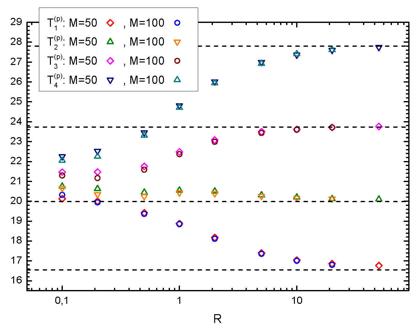
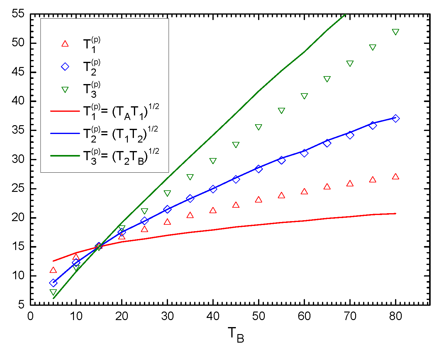
In order to better understand the dependence of our theoretical results on the parameter R, we have performed numerical simulations of the system for different values of R. From the previous remark, we expect to have an improvement of the agreement between the numerical results and the analytical predictions by increasing R. In Figure 5, we compare the piston temperature in a 4-piston system with theoretical predictions from Equation (26), finding a very good agreement for large values of R. This shows that the total mass of the gas contained in a box has to be larger than the mass of the piston, in order for the kinetic theory presented in the previous section to be accurate.

6. Conclusions

We have studied a generalized piston in contact with two thermal baths at different temperatures. This system represents a simple but interesting case where the emergence of Fourier’s law from a microscopic mechanical model can be studied. We have presented a kinetic theory treatment inspired by an approach à la Smoluchowski, and we have investigated the range of validity of these results with molecular dynamics numerical simulations. We have found that, in order for the theory to be accurate, the ratio $R=mN/M$ should be large enough, namely the total mass of the gas in each compartment should be greater than that of the single piston.

We have considered ideal gas in our model, but we do not expect that the introduction of short-range interactions among gas particles, at least in not too dense cases, leads to significant differences in the behavior of the system. An interesting, non-trivial, future line of research in this model is the study of the relaxation to the steady state and the dynamical properties of the system, focusing on correlation and response functions.

References

1. Lepri, S.; Livi, R.; Politi, A. Thermal conduction in classical low-dimensional lattices. Phys. Rep. 2003, 377, 1–80. [Google Scholar] [CrossRef]
2. Garrido, P.L.; Hurtado, P.I.; Nadrowski, B. Simple one-dimensional model of heat conduction which obeys Fourier’s law. Phys. Rev. Lett. 2001, 86, 5486. [Google Scholar] [CrossRef] [PubMed]
3. Dhar, A. Heat conduction in the disordered harmonic chain revisited. Phys. Rev. Lett. 2001, 86, 3554. [Google Scholar] [CrossRef] [PubMed]
4. Lepri, S.; Livi, R.; Politi, A. On the anomalous thermal conductivity of one-dimensional lattices. EPL 1998, 43, 271–276. [Google Scholar] [CrossRef]
5. Giardinà, C.; Livi, R.; Politi, A.; Vassalli, M. Finite thermal conductivity in 1D lattices. Phys. Rev. Lett. 2000, 84, 2144. [Google Scholar] [CrossRef] [PubMed]
6. Eckmann, J.P.; Young, L.-S. Temperature profiles in Hamiltonian heat conduction. EPL 2004, 68, 790–796. [Google Scholar] [CrossRef]
7. Eckmann, J.P.; Young, L.-S. Nonequilibrium energy profiles for a class of 1-D models. Commun. Math. Phys. 2005, 262, 237–267. [Google Scholar] [CrossRef]
8. Salazar, A.; Larralde, H.; Leyvraz, F. Temperature gradients in equilibrium: Small microcanonical systems in an external field. Phys. Rev. E 2014, 90, 052127. [Google Scholar] [CrossRef] [PubMed]
9. Gaspard, P.; Gilbert, T. Heat Conduction and Fourier’s Law by Consecutive Local Mixing and Thermalization. Phys. Rev. Lett. 2008, 101, 020601. [Google Scholar] [CrossRef] [PubMed]
10. Gaspard, P.; Gilbert, T. Heat conduction and Fourier’s law in a class of many particle dispersing billiards. New J. Phys. 2008, 10, 103004. [Google Scholar] [CrossRef]
11. Olla, S.; Sasada, M. Macroscopic energy diffusion for a chain of anharmonic oscillators. Probab. Theory Relat. Fields 2013, 157, 721. [Google Scholar] [CrossRef]
12. Crosignani, B.; Di Porto, P.; Segev, M. Approach to thermal equilibrium in a system with adiabatic constraints. Am. J. Phys. 1996, 64, 610–613. [Google Scholar] [CrossRef]
13. Gruber, C.; Piasecki, J. Stationary motion of the adiabatic piston. Physica A 1999, 268, 412–423. [Google Scholar] [CrossRef]
14. Gruber, C.; Pache, S.; Lesne, A. Two-time-scale relaxation towards thermal equilibrium of the enigmatic piston. J. Stat. Phys. 2003, 112, 1177–1206. [Google Scholar] [CrossRef]
15. Gruber, C.; Lesne, A. Hamiltonian model of heat conductivity and Fourier law. Physica A 2005, 351, 358–372. [Google Scholar] [CrossRef]
16. Van den Broeck, C.; Kawai, R.; Meurs, P. Microscopic analysis of a thermal Brownian motor. Phys. Rev. Lett. 2004, 93, 090601. [Google Scholar] [CrossRef] [PubMed]
17. Cencini, M.; Palatella, L.; Pigolotti, S.; Vulpiani, A. Macroscopic equations for the adiabatic piston. Phys. Rev. E 2007, 76, 051103. [Google Scholar] [CrossRef] [PubMed]
18. DelRe, E.; Crosignani, B.; Di Porto, P.; Di Sabatino, S. Built-in reduction of statistical fluctuations of partitioning objects. Phys. Rev. E 2011, 84, 021112. [Google Scholar] [CrossRef] [PubMed]
19. Sarracino, A.; Gnoli, A.; Puglisi, A. Ratchet effect driven by Coulomb friction: the asymmetric Rayleigh piston. Phys. Rev. E 2013, 87, 040101(R). [Google Scholar] [CrossRef] [PubMed]
20. Cerino, L.; Gradenigo, G.; Sarracino, A.; Villamaina, D.; Vulpiani, A. Fluctuations in partitioning systems with few degrees of freedom. Phys. Rev. E 2014, 89, 042105. [Google Scholar] [CrossRef] [PubMed]
21. Cerino, L.; Puglisi, A.; Vulpiani, A. Kinetic model for the finite-time thermodynamics of small heat engines. Phys. Rev. E 2015, 91, 032128. [Google Scholar] [CrossRef] [PubMed]
22. Tehver, R.; Toigo, F.; Koplik, J.; Banavar, J.R. Thermal wall in computer simulations. Phys. Rev. E 1998, 57, R17–R20. [Google Scholar] [CrossRef]
Figure 1. Sketch of the system.
Entropy 19 00350 g001
Figure 2. Piston temperatures for a 3-piston system, with parameters T A = 15 , N = M = 100 , m = 1 , L = 1 .
Entropy 19 00350 g002
Figure 3. Temperature profiles for a 22-piston system with R = 1 and R = 10 . Other parameters are T A = 15 , T B = 30 , M = 50 , m = 1 , L = 1 .
Entropy 19 00350 g003
Figure 4. Probability distribution function of the velocities ϕ L ( v ) ( ϕ R ( v ) ) of the particles colliding with the first piston from the left (right), for a system with n = 2 . The curves, red and blue, are respectively: ϕ L = m k B T L e v 2 / k B T L v θ ( v ) and ϕ R = m k B T R e v 2 / k B T R v θ ( v ) , where T L = 15.0 and T R = 21.6 are the temperatures of the gas on the left and on the right with respect to the first piston. Other parameters are: T A = 15 , T B = 30 , N = 100 , M = 100 , m = 1 , n = 2 , L = 1 .
Entropy 19 00350 g004
Figure 5. Piston temperatures for a 4-piston system as a function of R. Dashed lines are the theoretical predictions. Other parameters are T A = 15 , T B = 30 , m = 1 , L = 1 .
Entropy 19 00350 g005