A Sparse Multiwavelet-Based Generalized Laguerre–Volterra Model for Identifying Time-Varying Neural Dynamics from Spiking Activities


1
School of Automation Science and Electrical Engineering, Beihang University, Beijing 100191, China
2
Department of Mathematics, Texas A&M University at Qatar, Doha 23874, Qatar
3
Department of Electronic Engineering, City University of Hong Kong, Hong Kong, China
*
Authors to whom correspondence should be addressed.
Entropy 2017, 19(8), 425; https://doi.org/10.3390/e19080425
Submission received: 13 July 2017
/
Revised: 7 August 2017
/
Accepted: 18 August 2017
/
Published: 20 August 2017
(This article belongs to the Special Issue Entropy in Signal Analysis)
Abstract
:Modeling of a time-varying dynamical system provides insights into the functions of biological neural networks and contributes to the development of next-generation neural prostheses. In this paper, we have formulated a novel sparse multiwavelet-based generalized Laguerre–Volterra (sMGLV) modeling framework to identify the time-varying neural dynamics from multiple spike train data. First, the significant inputs are selected by using a group least absolute shrinkage and selection operator (LASSO) method, which can capture the sparsity within the neural system. Second, the multiwavelet-based basis function expansion scheme with an efficient forward orthogonal regression (FOR) algorithm aided by mutual information is utilized to rapidly capture the time-varying characteristics from the sparse model. Quantitative simulation results demonstrate that the proposed sMGLV model in this paper outperforms the initial full model and the state-of-the-art modeling methods in tracking performance for various time-varying kernels. Analyses of experimental data show that the proposed sMGLV model can capture the timing of transient changes accurately. The proposed framework will be useful to the study of how, when, and where information transmission processes across brain regions evolve in behavior.
1. Introduction
Modeling of information transmission processes across brain regions, including spike generation and synaptic transmission, is challenging because neurobiological processes can be nonstationary [1,2]. For example, studies establish that the synaptic plasticity, with specific forms of long-term potentiation (LTP) and long-term depression (LTD), occur in response to specific input patterns, which can be indicated as the system nonstationarity. However, tracking of the changes for such time-varying functional connectivity on the level of neural ensembles is still challenging [3] due to the potential nonstationary properties.
Generally, three major classes of system identification methods have been applied to the study of the time-varying neural system. The first class of the nonstationary systems modeling method is the data-driven artificial neural networks (ANNs), which have been widely applied to various fields, including speech recognition [4], forecasting [5], as well as nonstationary or nonlinear system modeling [6]. However, the multiple hidden layers and the nodes in the networks structure are usually difficult to interpret. The second class of time-varying parametric estimation approaches is based on the adaptive filtering strategy, such as the steepest descent algorithm [7], stochastic gradient algorithms [8], Kalman filter and its variants [9]. The adaptive filter algorithms for the spike train data update the model parameters iteratively according to the difference between the occurrence of a real spike and the estimated spiking firing probability [10], which has an advantage in online estimation of a model that represents the best fit to an unknown neural system. However, if the model coefficients changed abruptly, adaptive filters might be incapable of capturing the transient properties of a time-varying system due to the convergence time taken in the adaptive filters method [11].
The third class is the basis function expansion method where the unknown time-varying parameters are projected onto a set of predefined basis functions. By this means, the time-varying identification problem can be transformed into an expansion-based time-invariant parametric modeling scheme, with remarkable reduction in the number of the coefficients to be estimated. A variety of basis functions can be utilized under this strategy, including the Walsh function [12], Chebshev basis [13], Laguerre polynomials [14], Legendre series [15], and wavelets [16,17]. Each family of basis functions should be considered based on its unique fit to the kernel shape if the number of basis functions to be used is limited. For example, the Chebshev basis and the Legendre polynomials both perform well in tracking smoothly or slowly changing parameters [13], while the Walsh and Haar basis functions are appropriate for tracking abrupt time-varying parameters [18]. Towards the applicability to a dynamical system with spike train inputs and outputs, the Chebshev basis expansion technique has been tested [19]. However, an unknown neural system can involve multitudes of time-varying dynamics, where both smooth and abrupt changes can be found simultaneously. The Chebshev basis expansion may be insufficient to capture the potential diverse time-varying properties effectively. Instead, we propose the use of a wavelet basis function, which is localized both in the time and frequency domain [20], can be effectively utilized to represent a sharp or slow variation vanishing outside a short time interval [21,22]. Li et al. previously combined the cardinal B-splines basis function with a block least mean square algorithm to track both slow and rapid changes of coefficients effectively in time-varying linear systems [23,24]. The team later extended this method to the identification of nonlinear time-varying systems and obtained satisfactory results of tracking time-varying variations from EEG nonstationary data [25].
A biological neural network commonly exhibits small-world properties where the neurons are not fully connected [26,27]. Commonly, the direct utilization of the basis function expansion method based on all input spiking signals can easily suffer from an overfitting problem due to the spurious input connectivity. Regularization is crucial for achieving functional sparsity at the global levels, which has been increasingly applied to solve the ill-posed or overfitting problems in the statistics and machine learning field [28]. In the context of the sparsity in neural connectivity, the regularization method is also very popular to process the issue of the sparse connectivity [29]. Various regularization approaches, such as the least absolute shrinkage and selection operator (LASSO) [30], the smoothly clipped absolute deviation (SCAD) [31], group LASSO [32], and group ridge [33] have been employed to obtain sparse representations. For example, Song et al. implemented a group LASSO to capture the sparsity of a neural system [34]. However, existing studies only focused on a time-invariant system, while there is a lack of reliable method for the regularized estimation of the time-varying system in nature. In addition, our previous work indicated that the multiwavelet-based time-varying generalized Laguerre–Volterra model can be used to track both slow and rapid changes of time-varying parameters simultaneously for the spiking train data [24], while it may fall into the dilemma of overfitting in the case that the neural system is rather sparsely connected. Therefore, we may integrate both the group LASSO and the multiwavelet basis expansion method in a unified framework to include their advantages (e.g., the group LASSO algorithm can eliminate the spurious input and capture the sparsity of a neural system, while the multiwavelet basis expansion method can effectively track both slow and rapid changes of time varying parameters simultaneously) and achieve an efficient and accurate estimation for the nonstationary spiking system.
In this paper, we propose a sparse multiwavelet-based generalized Laguerre–Volterra (sMGLV) modeling framework to identify the underlying nonstationary sparse neuronal connectivity by observing the input and output spike trains only. The contributions of this paper are threefold. First, we address the problem of effective input selection by using a group LASSO regularization method in the analysis of the time-varying dynamics within a neural system. Second, in order to estimate the time-varying kernels quickly and accurately, we project the time-varying parameters in the sparse model onto a set of multiwavelet-based basis functions so that the time-varying parameters estimation problem can be tackled within the time-invariant regression scheme. Third, we utilize an effective forward orthogonal regression (FOR) aided by the mutual information (MI) criterion (FOR-MI) algorithm to determine and refine the model structure. The redundant model terms or regressors will be removed, and thus a compact model with good generalization performance is achieved. Particularly, the proposed sMGLV modeling approach can produce an optimal model structure to characterize the time-varying dynamical processes underlying the spiking system. The novel sMGLV framework integrates the group LASSO regularization algorithm and the multiwavelet basis expansion method in a unified framework to obtain an efficient and accurate estimation for the nonstationary spiking system. An obvious advantage of the proposed framework lies in its ability to track rapidly and even sharply time-varying processes on the condition that the neurons are not fully connected. Extensive simulation results demonstrate that the sMGLV model outperforms the existing state-of-the-art modeling methods in the identification of sparse time-varying neural connectivity. Redundant inputs can be effectively eliminated while more reliable kernel estimations can be obtained from a group of neural spiking signals. Experimental results show that the proposed method can track the changes of the functional connectivity in a real retinal neural spike train signals accurately.
2. Methodology
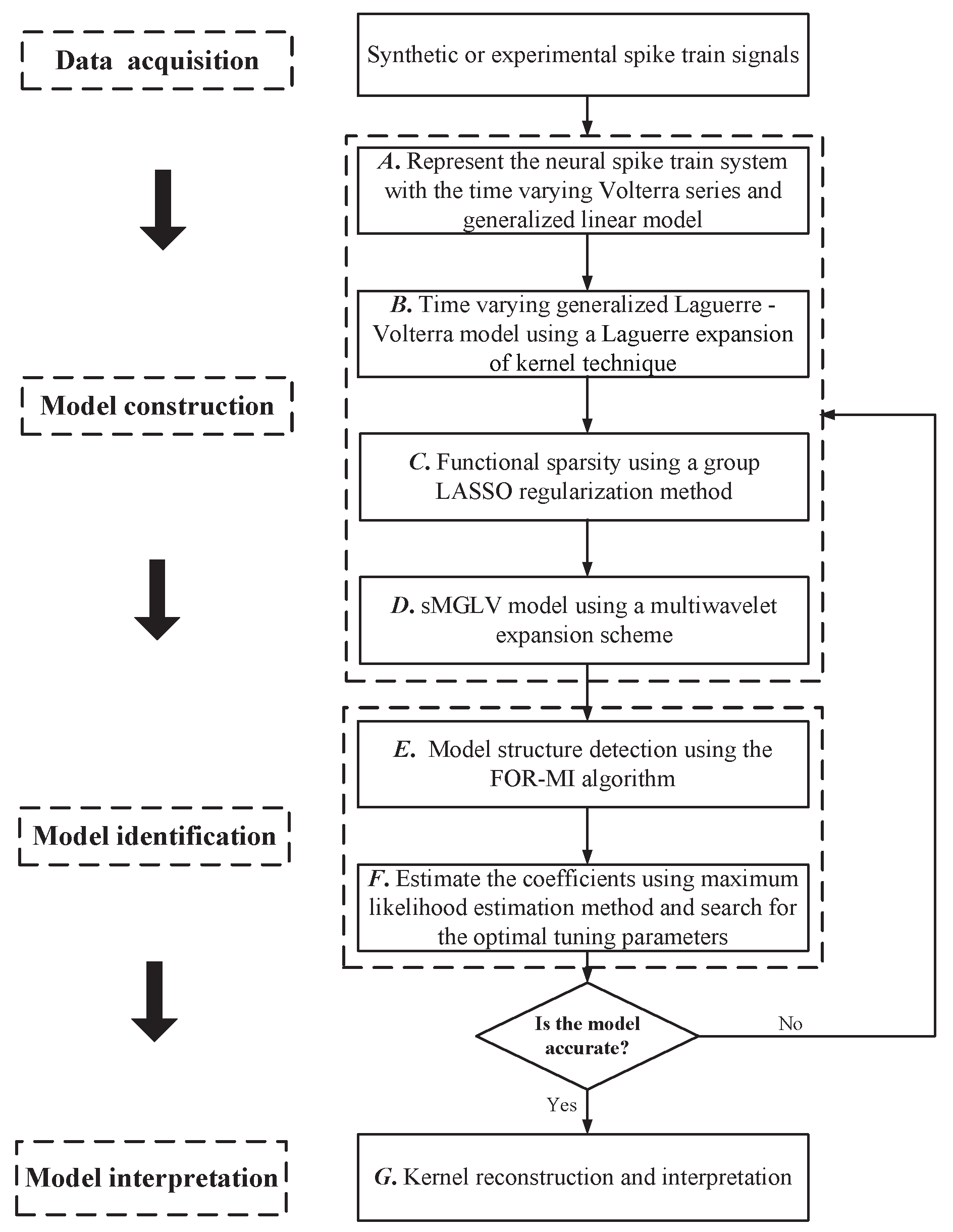
The schematic diagram for the proposed sMGLV framework is shown in Figure 1. The sMGLV model is implemented by using the Laguerre expansion of the kernel technique, the group LASSO regularization method, and the multiwavelet expansion scheme based on the time-varying Volterra series and generalized linear model, respectively. Furthermore, an effective FOR-MI algorithm provides an optimal model structure, where the expansion parameters are obtained with a maximum likelihood estimation method. Finally, the time-varying Volterra kernels are reconstructed for a biologically plausible description of the neural dynamics.
2.1. Time-Varying Generalized Volterra Model
Neural spiking activities can be viewed as point processes, represented as binary signals [35]. That is, 1 in the time series corresponds to when the spike is observed at the predefined time interval, and 0 otherwise [36]. The spiking activity of an output neuron depends on not only the current activities of other neurons, but also the spiking histories, which requires a dynamical model to capture a causal relationship [34]. Given the history of the input and output signals, the conditional probability of the action potential of the output signal can be expressed as follows [34]:
where y denotes the output signal, X represents the set of all the equivalent input signals and M is the memory length in the system. Note that , which contains the output signal y itself for the purpose of including the autoregressive effect of the preceding activities, namely, the total number for the input signals is , and the autoregressive effect from the preceding output can be written as for simplicity (Table 1).
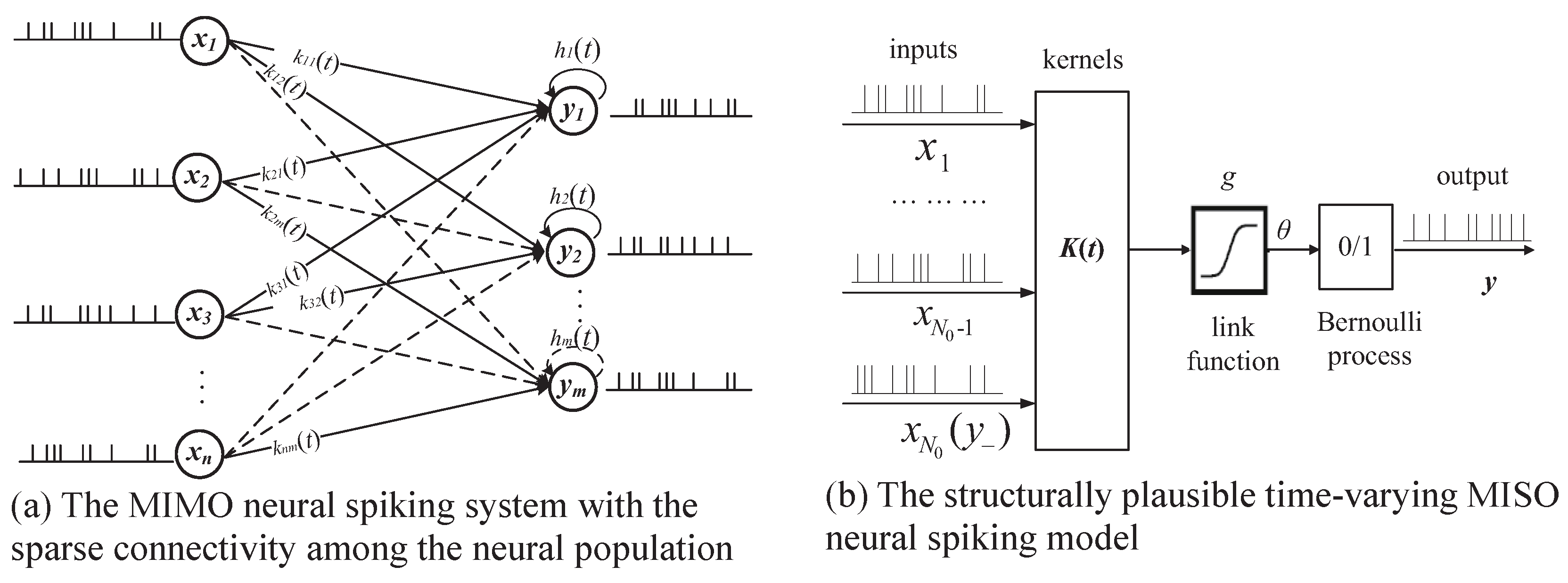
The input–output dynamics is represented by a multi-input, multi-output (MIMO) framework, which is decomposed into a series of structurally plausible multi-input, single-output (MISO) models. The structure for the time-varying MIMO and MISO neural systems for spiking data can be given in Figure 2. Note that a population of neurons in the network tend to be sparsely connected. An output is typically innervated by only a small subset of neurons in its input region and thus exhibits a high level of sparsity in nature.
The Voterra series expression has been widely used to represent the feedforward and feedback kernels in the context of the spiking neural system [34]. To describe the causal relationship between the input and output spiking probability, the generalized linear model with time-varying Volterra series is utilized as follows:
where is a scalar zeroth-order kernel function, and are first-order kernel functions describing the relationship between the output spiking probability and the n-th input. Here, is a known probit link function, which can be interpreted as a noisy threshold function that transforms the pre-threshold membrane potential to output spikes [36]. With the probit link function, Equation (2) can be rewritten in the form of the normal cumulative distribution function as follows [34]:
where the function erf is the Gaussian error function that can be defined by
2.2. Time-Varying Generalized Laguerre–Volterra Model
The memory length in the neurons may last for hundreds of milliseconds. If M is large, thousands of unknown coefficients have to be estimated for each input kernel in Equation (2). To alleviate computational complexity, Laguerre expansion decomposes the kernel functions into a set of weighted summation of the predefined orthogonal Laguerre basis functions:
where ) represents the l-th order Laguerre basis function, and denote time-varying Laguerre expansion coefficients of the n-th kernels. The total number of basis functions L has been chosen in the range of 3 to 15 based on previous experimental analyses [37]. L also determines the complexity for the Laguerre expansion model. Specially, a larger L can give rise to more model terms and increase the computationally complex, while a more accurate and good generalization model will be produced. The Laguerre basis function b employed here can be obtained iteratively by [38]:
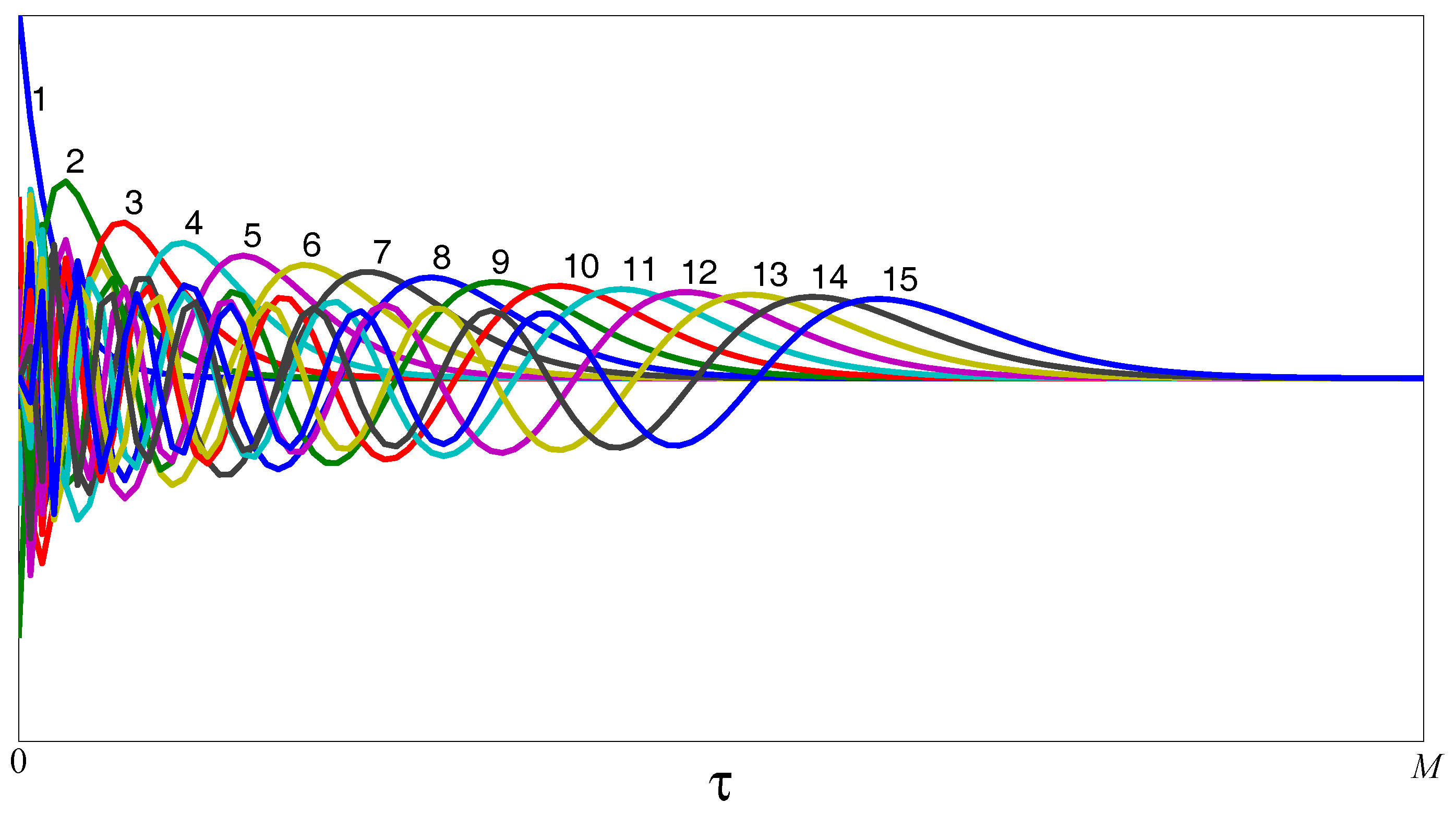
where is the Laguerre parameter (), which determines the exponential decaying rate of the Laguerre basis functions. The bigger the parameter is, the slower the Laguerre basis function decays, and a longer spread of significant non-zero values can be seen in the basis function [37]. The system kernels with longer memory may require a larger for efficient representation. Therefore, the proper selection of the parameter and L can effectively represent the time-varying system coefficients. Figure 3 shows the first 15 Laguerre basis functions, where the Laguerre parameters L equals 15 and equals 0.7. The basis function expands the entire system memory .
With input spike trains in X convolved with b, the convolved products v are represented by
The time-varying generalized Volterra model in Equation (2) can thus be rewritten by
where represent the coefficients of the Laguerre expansion of the respective kernels, as functions of time. The model described in Equation (8) forms the time-varying generalized Laguerre–Volterra (TVGLV) model. Given that the order of the Laguerre basis functions L is usually much smaller than the memory length M, the number of time-varying coefficients to be estimated can be largely reduced after the Laguerre expansion procedure.
2.3. Functional Sparsity Based on a Group Regularization Method
Nodes in biological neural network are not fully connected [26]. Namely, only a small subset of the given multiple input signals may connect to the signal recorded from the output neuron. However, a full Volterra kernel model constructed with all the observed signals described in Equation (2) or (8) does not capture the sparsity yet. Therefore, functional sparsity is introduced to the time-varying generalized Laguerre–Volterra model. Using a regularization approach, the functional sparsity can select the significant inputs by enforcing the estimated kernels of the redundant inputs to be zeroes.
Regularization approaches, including LASSO [30], SCAD [31], group LASSO [32] and group bridge [33], have been widely applied to simultaneous parameter estimation and variable selection. The former two methods can achieve individual coefficient selection, while the latter two can produce a sparse set of groups. In the TVGLV model, the Laguerre approximation coefficients can be grouped with regard to the associated input signals, for example, can be assigned to the same group because they all belong to the n-th input. Given this group setting, functional sparsity then refers to the occurrence that the estimation for several groups of Laguerre expansion coefficients all remain zero-valued. Therefore, a group LASSO regularization method based on the minimization of the sum of squared errors is utilized for a sparse TVGLV model. The group LASSO penalty term can be consisted as a hybrid of -penalty and -penalty: within the groups, it shrinks (but does not select) the coefficients with the -norm regularization; across groups, it selects the groups in a -norm regularization fashion. Specifically, the expression for the group LASSO penalty utilized here can be given as:
where the subscript “2” is the -norm regularization within the groups, and the super-script “1” represent the -norm regularization across the groups. represents the mean value of time-varying Laguerre expansion coefficients during the whole data length, and can be estimated by using the maximum likelihood estimation method in Equation (8). The group LASSO regularization criterion can thus be represented by:
where is a regularization parameter that controls the sparsity degree of the model, i.e., a larger value of yields sparser results of the coefficients. A wide range of from to is explored. For each , deviance is obtained from a cross-validation strategy. The with the smallest deviance and the corresponding set of C are used to find out the spurious inputs. For example, a redundant input can be determined if all the Laguerre expansion coefficients belonging to its group equal to zeroes.
Suppose that the selected Laguerre expansion coefficients are , , the associated inputs can thus be expressed as . According to Equation (8), the sparse TVGLV model can be written as follows:
By means of the group LASSO regularization method, the functional global sparsity can be achieved and the neural connectivity can thus be accurately represented. Furthermore, time-varying parameters can be efficiently estimated by using the following multiwavelet-based expansion scheme.
2.4. Sparse Multiwavelet-Based Generalized Laguerre–Volterra Model
Previous work has illustrated that expanding time-varying coefficients onto a set of basis functions can largely improve the tracking performance of the time-varying model and reduce the model complexity because the TVGLV model can be transformed into a time-invariant regression model [19]. The multiwavelet basis functions are usually employed to approximate the time-varying parameters because of their good approximation performance in tracking both fast and slowly varying trends regardless of the a priori knowledge of nonstationary processes. Thus, we can project time-varying Laguerre expansion coefficients in the sparse TVGLV model onto a set of multiwavelet basis functions, which can be yielded the following formula:
where are the wavelet basis functions, with the shift indices , , wavelet scale j and the wavelet order m, respectively. , with are the time-invariant coefficients in the multiwavelet-based model expansion. T is the length of observed data. Multiwavelet basis functions are combined with a series of wavelet basis functions from different orders. It should be noted that wavelet basis functions of lower orders tend to perform well on the change of signals with sharp transients, while the wavelet basis functions of higher orders tend to perform well on the change of signals smoothly. Multiwavelet basis functions can thus be adopted to approximate time varying coefficients with both rapid and slow variations. Considering the cardinal B-spline basis functions to be completely supported with excellent approximation properties [17], can take the form of the B-spline basis function with the m-th order ():
where the variable is normalized to and shift indices k satisfies . The scale j determines the resolution, namely, a larger j leads to a higher resolution, and also a bigger of the computation complexity. For most nonlinear dynamical modelling problems for the neural spiking data, scale j of 3, and the wavelets of order selected from are usually adequate, which can be graphically illustrated in Figure 4. The detailed discussions on the selection of proper scale j and the associated wavelet order can be found in [39].
By substituting Equation (13) into Equation (11), the sparse multiwavelet-based generalized Laguerre- Volterra model is given below:
where , are the time-invariant coefficients to be estimated. For simplification, new variables can be defined by:
Substituting Equation (15) into Equation (14) obtains
where are the full model terms in the sparse mutliwavelet-based TVGLV expansion model. Hence, the original time-varying model described in Equation (11) is now transformed into a time-invariant regression model, which enables the coefficient estimation problem to be solved within the maximum-likelihood framework.
2.5. Model Structure Selection
The multiwavelet-based basis function expansion model in Equation (16) may involve myriad candidate terms or regressors if the model parameters L, J, m and N are large, which can easily result in an overfitting problem. Thus, determination of the significant terms or regressors to be included in the final identified model is crucial prior to estimating time-invariant expansion coefficients.
LASSO-related penalized regression methods are popular for variables or terms selection studies [30,40,41]. However, the LASSO algorithm cannot guarantee consistency in the model term selection, and noisy terms can be occasionally selected [42]. Nonetheless, the computation of such methods is demanding considering that the number for the candidate terms in the expansions is large [42]. By contrast, the orthogonal-least-squares-type methods can obtain unbiased estimates [43]. The forward orthogonal regression (FOR) algorithm aided by mutual information criterion (MI) (FOR-MI) is an efficient and widely-used method in respect of model structure selection [44]. Thus, the FOR-MI method has been adopted to select significant model terms in the neural dynamical system from spike train data, which can effectively achieve local sparsity for the model structure. Consider two random discrete variables and , the MI criterion is used to measure the reduction in the uncertainty of due to the knowledge of , which can be defined as [45]:
where and represent the marginal probability density functions, and denotes the joint probability density function.
Given the binary characteristics of input and output data, the model structure detection algorithm based on the full model in Equation (16) can be described as follows:
Step 1. Combine the output observation y and the full model candidates , the maximum likelihood estimator can be estimated by using a generalized linear model fitting method. The output spike probability can further be obtained using Equation (16). Assume , to be a vector of the measured outputs with T time instants.
Step 2. The model terms are candidates for the first selected significant terms . Let and
The first significant term can be selected as , and is selected with both and . The error-to-signal ratio (ESR) is given as the search termination criterion below:
Step 3. The rest of the model terms form the candidate terms for . Let
and we can obtain
Then, the second term can be selected as , and is selected with both and . ESR is represented by
Step 4. Subsequent significant terms can be selected in the same way step by step until terminated at the p-th step when some certain criteria is satisfied. A generalized cross-validation (GCV) is used to determine model size, which can be expressed as [44]:
where is the mean square error (MSE) corresponding to the optimal model with the p significant terms selected. The effective number of model terms can thus be obtained with a minimum GCV value. Through the model structure detection procedure, the significant model terms can be selected from a large number of redundant model terms and therefore a parsimonious model can be obtained.
2.6. Parameter Estimation and Tuning Parameter Optimization
Assuming that the significant model terms selected using the FOR-MI algorithm can be given as , and the associated time-invariant expansion coefficients can be easily estimated by using a maximum-likelihood method. The log likelihood function can be expressed as follows:
The log-likelihood can thus be defined by:
Plugging the selected model terms to approximate in the above equation yields an approximation of l. The criterion is a function of basis function coefficients and denoted by . The maximizer of is the maximum likelihood estimator (MLE) that is represented as , which can be calculated using the standard iterative reweighted least-squares method.
The optimization of the tuning parameters, including the , are critical for achieving an accurate and efficient model. The well-known Bayesian information criterion (BIC) is employed to determine the proper tuning parameters, which can be calculated as follows:
where is the estimated coefficients corresponding to a certain set of tuning parameters. The optimal tuning parameters of the proposed sparse multiwavelet-based generalized Laguerre–Volterra model can be determined with the minimum of the BIC value.
2.7. Kernel Reconstruction and Interpretation
With the proper model terms selected and the corresponding time-invariant expansion coefficients estimated, a parsimonious model can therefore be achieved through a kernel reconstruction and normalization procedure.
The Laguerre expansion coefficients can be calculated using Equation (12). The Voterra kernels for the significant inputs can thus be reconstructed as follows:
Towards the interpretation, the kernel functions can further be normalized by the zeroth-order kernel as
where the threshold for the spike generating is set to be 1, and the was set to be −1.
As to the interpretation for the reconstructed model, is the conditional probability of the action potential of the output signal, and with a probit link function can be regarded as the membrane potential of the output neuron. is the postsynaptic potential in the output neuron elicited by the n-th input neuron when n is within , and the output neuron itself when n equals to . Inputs with all zero-valued kernels is identified as the redundant inputs.
3. Simulation Studies
Synthetic spike train data was generated from known systems to study the tracking performance of both the rapid and gradual changing kernels using the proposed sMGLV approach. Simulated system shown in Figure 5, Figure 6 and Figure 7 is an 8-input and 1-output spiking neural system where the first four kernel functions () undergo step changes and the other two kernels () undergo slower gradual changes concurrently. To make the tracking task more difficult, the last two kernels () are designed to be zeroes as redundant inputs to the spiking neural system. The transient changes for all step changing kernels occur at 400 s. In particular, the amplitudes of and are doubled, while the amplitudes of and are decreased by half. To test the concurrent tracking performance in identifying gradual changes, and are linear time-varying kernels with different slopes, as shown in Figure 6 and Figure 7. Additionally, the feedback kernel from the preceding output signal can be denoted by , and is set to be time-invariant in this simulation. The zeroth-order kernel, i.e., the baseline, is set as a constant 0. Specific shapes for different kernels are shown in Figure 5. The input signals are eight independent Poisson random spike trains with a mean firing rate of 10 Hz. The simulation length is 800 s with a bin size of 2 ms. Given the input spike trains and the known kernels defined in this simulation, the conditional probability of the output signal can be generated by using Equation (3), which can be used to produce the output spike trains at different times through a Bernoulli process.
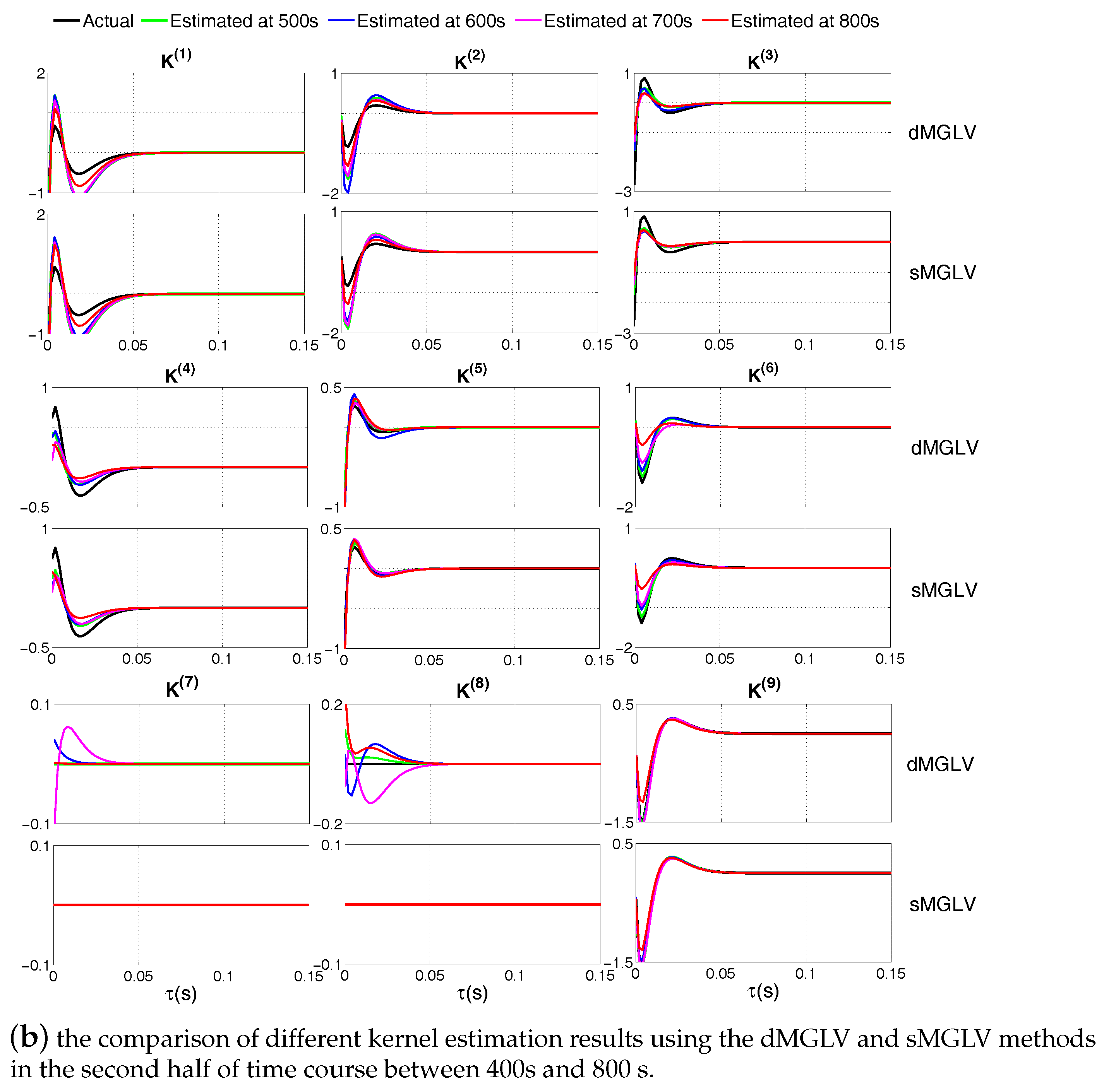
Using the input and output spike train data, kernel functions can be estimated by the proposed sMGLV method. As a comparison, the tracking result of a direct multiwavelet-based modelling method (dMGLV) without removing the redundant inputs is also provided to estimate the time-varying dynamical system in order to verify the effectiveness of the proposed approach. The tuning parameters utilized are the same for two compared methods according to Equation (27). Figure 5 illustrate the recovered kernel functions during different time courses using the dMGLV model and the proposed sMGLV model. The x-axis in the figure represents the time lag between the previous input events and the present time, and the y-axis indicates the amplitude of kernels. The true kernels are shown in black lines, and the estimated kernels over different time evolution can be displayed in different colors. Specifically, Figure 5a represent the estimated kernels in the first half of the simulation time course (the first 400 s) using two different methods, while Figure 5b represent the estimated kernels in the second half of the simulation time evolution (the last 400 s) using two different methods. The experiment results clearly indicate that the dMGLV model cannot capture global sparsity, that is, unable to recognize the redundant inputs. The dMGLV modeling method estimates spurious inputs even for zero-valued kernel functions, which is shown in Figure 5. In contrast, the proposed sMGLV model can accurately recognize all redundant inputs. As for the non-zero kernel functions, both dMGLV and sMGLV modeling methods can estimate the accurate kernel shapes accurately. Particularly, the proposed sMGLV model can effectively eliminate the redundant inputs, and therefore achieve a more reliable and accurate kernel estimation for the neural spiking system.
We have also compared the tracking performance for both the rapid and gradual changing kernels in the whole simulation data length. As shown in Figure 6 and Figure 7, apart from the proposed method, the stochastic state point process filtering algorithm (SSPPF), SSPPF with the group LASSO algorithm (sSSPPF), and the dMGLV model are also utilized for comparison. Specifically, Figure 6 shows the actual and estimated kernels over the time evolution, where the x-axis denotes the simulation time, the y-axis represents the time lag lasting from the previous input events to the present time, and the amplitudes of the kernel functions are color-coded. Additionally, Figure 7 illustrates the tracking results of the peak values of the estimated nonstationary feedforward and time-invariant feedback kernels using four different methods, where the x-axis represents simulation time course, and the y-axis indicates the kernel amplitudes for different spike train signals. The goodness-of-fit is quantitatively evaluated by comparing the mean absolute error (MAE) and normalized root mean square error (RMSE). The MAE and RMSE of the kernel estimates for the simulation spike train data, with respect to the corresponding true values, are estimated and shown in Table 2. Compared with the SSPPF, sSSPPF and the dMGLV model, the MAE and RMSE for the proposed sMGLV are much smaller. The MAE and RMSE of the peak amplitudes for the kernel are defined by
where and represent the peak amplitudes of the actual and estimated kernels at different times, respectively. Table 2 statistically confirms the better performance of the proposed sparse multiwavelet-based TVGLV model. Compared with the conventional SSPPF, the SSPPF with the group LASSO and the direct multiwavelet-based modeling method, the above simulation results indeed show that the proposed approach possesses much higher accuracy in kernel estimates.
Experiment results show that four estimation methods can all track the nonstationary kernels with step or linear changes. Although the SSPPF can roughly track the changes of the significant kernels, its estimates for the insignificant inputs are poor due to its inability in identifying the redundant model inputs. By contrast, the sSSPPF method can firstly remove the redundant inputs and provide relatively satisfactory tracking results of time-varying kernels by eliminating the disruptions from the redundant inputs simultaneously. However, considering the deficiency of the convergence rate for the adaptive filter methods, the sSSPPF cannot accurately capture the transient properties of the jump or abrupt time-varying processes. The dMGLV method, which established under the multiwavelet-based expansion framework, outperforms the SSPPF-type methods in the respect of tracking results of time-varying kernels with both rapid and gradual changes over time evolution. Nevertheless, the parametric modeling method without considering the sparsity condition can also produce spurious kernels generated by the redundant model inputs. The proposed sMGLV can instead provide optimal estimations and be consistent with the identification of the sparse time-varying neural connectivity, where the redundant inputs can be effectively eliminated and more reliable kernel estimations can be obtained from a group of neural spiking signals. Therefore, the proposed sMGLV framework can remarkably improve the tracking performance of time-varying kernels from time-varying dynamical systems based on spiking activities, and can be generally applied to the analysis for the real nonstationary neural functional connectivity.
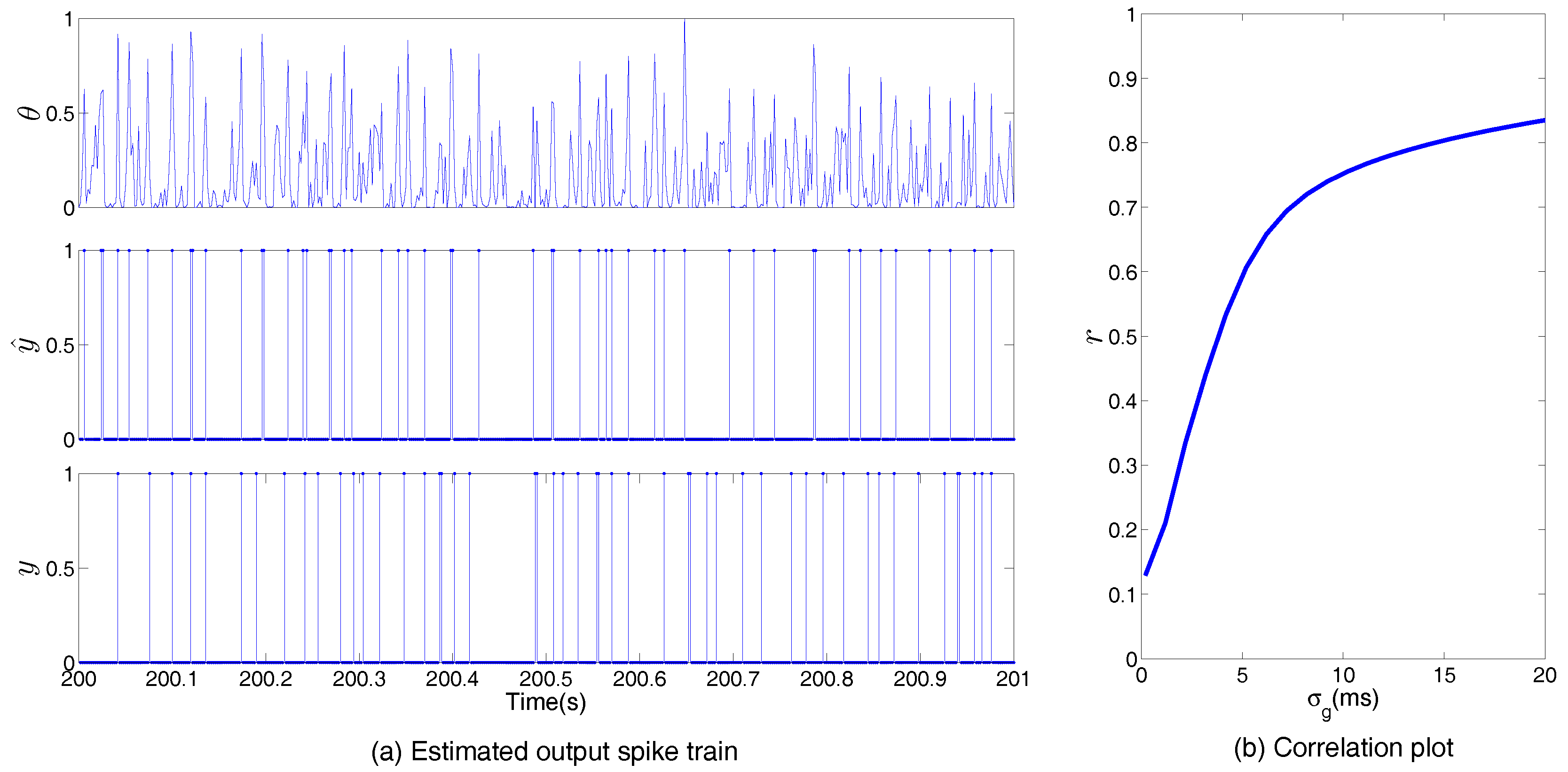
The estimated model under the proposed sGLMV framework can be further validated using the correlation plot for the estimated and actual output spike train. Figure 8a shows the estimated and actual output spike trains based on identical input spiking signals. The pre-threshold membrane potential was firstly calculated from the input spike trains (X) and the estimated kernels () using the proposed sMGLV model. Firing probability intensity () for the output was then obtained using the Gaussian error function in Equation (3) (Figure 8a, first row). The estimated output spike train () is finally obtained through a threshold procedure (Figure 8a, second row). The corresponding actual spike train (y) is also given in the third row in Figure 8a. Considering the stochastic nature of the model, the similarities between the estimated output spike train and the actual output spike train can be quantified with correlation plot (Figure 8b). Noted that the point-process signals and y are firstly convolved with a Gaussian kernel with standard deviation , and thus smoothed to continuous signals and , respectively. The correlation coefficient r is defined as follows [36]:
It shows that the proposed sMGLV model can generate output highly correlated with the actual output for a large range of standard deviation , and further validates the effectiveness of the proposed framework.
Results of additional intensive simulations have validated the advantages of the proposed sMGLV model over the state-of-the-art methods with respect to the identification of sparse time-varying neural connectivity. The proposed method can first select the significant inputs to avoid the estimation error produced by the redundant ones; then, both the gradual and rapid changes of the time-varying kernels can be tracked rapidly and accurately by using the sparse multiwavelet-based modeling framework.
4. Application to Functional Connectivity Analysis of Retinal Neural Spikes
The proposed sMGLV model can be generally applied to identify the functional connection from the experimental spiking train data. A set of spontaneous retinal spike train recordings has been used to illustrate and reveal the potential properties of the neural dynamics [46]. The dataset contains 512 electrodes recordings from retina of rats. The spontaneous spike trains were recorded simultaneously for 1000 s, with a sampling rate of 20 kHz and a bin size of 2 ms. In this experiment example, the system is composed of four inputs and one output. Utilizing the proposed modeling method, dynamics of four feedforward and one feedback kernels can be estimated during the time course.
Similar to the previous simulated example, the order for the B-splines basis function were adopted from 2 to 5 to construct the sMGLV model based on the spike trains. The tuning parameters are optimized using Equation (26), and thus both the optimal Laguerre parameter and the Laguerre basis number are 0.83 and 11, respectively. The regularization parameter in the group LASSO can be obtained using a cross validation method introduced in the Section C. A group LASSO with the B-splines expansion method is applied to the experimental spiking data to reveal the potential properties underlying the retinal neural system. The parsimonious model structure is produced with a FOR-MI algorithm and the expansion parameters are obtained with a maximum likelihood estimation method.
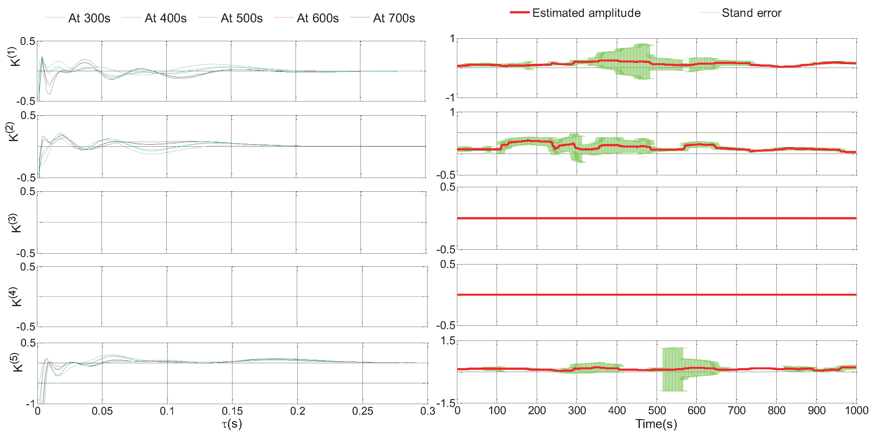
Figure 9 shows the reconstructed kernel results using the proposed sMGLV method over the time course. Specifically, the left figure in Figure 9 illustrates the estimated kernels at different time (i.e., 300 s, 400 s, 500 s, 600 s, 700 s), where the x-axis represents time lag between the previous input events and the present time, and the y-axis stands for the amplitudes of kernels. Experimental results show that the kernels for the first and second input spike train signals (i.e., and ) are nonzero, and thus are significant inputs, while the kernels of the third and fourth input spike train signals (i.e., and ) are yielded to be zero-valued for the whole system memory, and therefore deemed to be insignificant inputs. The sMGLV model can effectively identify the sparsity in the experimental system. Owing to eliminating the spurious inputs, the kernels for significant inputs can be estimated more accurately and are shown to keep the stable estimation results. The right figure in Figure 9 demonstrates the peak amplitudes and their corresponding stand deviation of different kernels across the experimental time in the spiking system, where the red lines represent the changes of the peak amplitudes over time and the green shade indicates the standard deviation for the amplitudes of the estimated kernels. Both of the peak amplitudes and their corresponding stand deviation can be easily derived based on the time-invariant expansion coefficients through Equations (12), (27) and (28). The peak amplitudes describe the changes for the estimated kernels during the experimental time, while the standard deviation accounts for the fluctuation ranges for the peak values. The experimental results in the right figure illustrate that the peak amplitudes for the significant inputs (i.e., and ) keep varying over time, which indicates the significant time-varying connection strength. These results demonstrate the applicability of the proposed sMGLV model framework to the real experimental data.
5. Conclusions
A novel sMGLV modeling framework has been formulated for the identification of time-varying neural dynamics from spiking activities. The proposed framework has three distinct advantages compared to the state-of-the-art modeling methods. First, in terms of the sparse neural connectivity, the proposed sMGLV modeling framework combines the Laguerre expansion technique with the group LASSO algorithm to realize a global sparsity, where spurious inputs can be effectively eliminated by enforcing the Laguerre expansion coefficients to be zero. Second, the proposed sMGLV modeling scheme projects the time-varying coefficients onto a set of multiwavelet-based basis functions. By this means, the time-varying modeling problem can be converted into a time-invariant regression problem, and further the tracking performance of time-varying models is improved. Third, for the issue of model overfitting, the proposed sMGLV model employs a FOR-MI method to select the significant terms and removes the redundant ones efficiently, and a satisfactory sparse model with good generalization performance is finally produced. Numerical simulation verified the effectiveness of the proposed modeling scheme in identifying the changes of the time-varying kernels. Its application to a real retinal spike train recorded indicates that the proposed method can be applied to the real experimental data, and obtain a relatively faithful expression for the sparse functional connectivity among the neural population. Therefore, the proposed sMGLV model developed in this paper can provide an integrated computational framework for investigating nonstationary properties and track more general forms of dynamical changes in the sparsely connected neural network. It may better the understanding of the information transmission across brain regions during behavior.
Finally, it should be noted that the mutliwavelet-based basis expansion scheme proposed here could be generally applied to kernels with time-varying weights while using different basis functions, such as Kautz filters [47], to capture the kernel shapes.
Acknowledgments
The work described in this paper was supported by a grant from the National Natural Science Foundation of China (61671042, 61403016 and 61403014), the Beijing Natural Science Foundation (4172037), as well as the Research Grants Council of the Hong Kong Special Administrative Region, China (Project No. CityU110813), the Open Fund Project of the Fujian Provincial Key Laboratory of Information Processing and Intelligent Control in Minjiang University (No. MJUKF201702), the Specialized Research Fund for the Doctoral Program of Higher Education (20131102120008), and the Project Sponsored by the Scientific Research Foundation for the Returned Overseas Chinese Scholars, State Education.
Author Contributions
Song Xu and Yang Li ran simulations, analyzed application results, and wrote the manuscript; Tingwen Huang offered useful suggestions for the manuscript preparation and writing; Rosa H. M. Chan offered the experimental data and analyzed application results.
Conflicts of Interest
The authors declare no conflict of interest.
References
- Chan, R.H.; Song, D.; Berger, T.W. Nonstationary modeling of neural population dynamics. Proeedings of the 31st Annual International Conference of the IEEE Engineering in Medicine and Biology Society, Minneapolis, MN, USA, 2–6 September 2009. [Google Scholar]
- Nasser, H.; Cessac, B. Parameter estimation for spatio-temporal maximum entropy distribu- tions: Application to neural spike trains. Entropy 2014, 16, 2244–2277. [Google Scholar] [CrossRef] [Green Version]
- Li, L.; Park, I.; Seth, S.; Sanchez, J.; Príncipe, J. Functional connectivity dynamics among cortical neurons: A dependence analysis. IEEE Trans. Neural Syst. Rehabil. Eng. 2014, 20, 18–30. [Google Scholar] [CrossRef] [PubMed]
- Dahl, G.; Yu, D.; Deng, L.; Acero, A. Context-dependent pre-trained deep neural networks for large-vocabulary speech recognition. IEEE Trans. Audio Speech Lang. Process. 2012, 20, 30–42. [Google Scholar] [CrossRef]
- Coulibaly, P.; Baldwin, C. Nonstationary hydrological time series forecasting using non-linear dynamic methods. J. Hydrol. 2005, 307, 164–174. [Google Scholar] [CrossRef]
- Iatrou, M.; Berger, T.W.; Marmarelis, V.Z. Modeling of nonlinear nonstationary dynamic systems with a novel class of artificial neural networks. IEEE Trans. Neural Netw. 1999, 10, 327–339. [Google Scholar] [CrossRef] [PubMed]
- Wang, J.; Wen, Y.; Gou, Y.; Ye, Z.; Chen, H. Fractional-order gradient descent learning of bp neural networks with caputo derivative. Neural Netw. 2017, 89, 19–30. [Google Scholar] [CrossRef] [PubMed]
- Sayed, A.H. Fundamentals of Adaptive Filtering; Wiley: Hoboken, NJ, USA, 2003. [Google Scholar]
- Seáñez-González, I.; Mussa-Ivaldi, F.A. Cursor control by kalman filter with a non- invasive body–Machine interface. J. Neural Eng. 2014, 11, 056026. [Google Scholar] [CrossRef] [PubMed]
- Eden, U.; Frank, L.; Barbieri, R.; Solo, V.; Brown, E. Dynamic analysis of neural encoding by point process adaptive filtering. Neural Comput. 2004, 16, 971–998. [Google Scholar] [CrossRef] [PubMed]
- Li, Y.; Liu, Q.; Tan, S.; Chan, R.M. High-resolution time-frequency analysis of eeg signals using multiscale radial basis functions. Neurocomputing 2016, 195, 96–103. [Google Scholar] [CrossRef]
- Zou, R.; Chon, K.H. Robust algorithm for estimation of time-varying transfer functions. IEEE Trans. Biomed. Eng. 2004, 51, 219–228. [Google Scholar] [CrossRef] [PubMed]
- Martel, F.; Rancourt, D.; Chochol, C.; St-Amant, Y.; Chesne, S.; Rémond, D. Time-varying torsional stiffness identification on a vertical beam using chebyshev polynomials. Mech. Syst. Signal Process. 2015, 54, 481–490. [Google Scholar] [CrossRef]
- Clement, P.R. Laguerre functions in signal analysis and parameter identification. J. Frankl. Inst. 1982, 313, 85–95. [Google Scholar] [CrossRef]
- Niedzwiecki, M. Identification of Time-Varying Processes; Wiley: New York, NY, USA, 2000. [Google Scholar]
- Su, W.C.; Liu, C.Y.; Huang, C.S. Identification of instantaneous modal parameter of time-varying systems via a wavelet-based approach and its application. Comput. Aided Civ. Infrastruct. Eng. 2014, 29, 279–298. [Google Scholar] [CrossRef]
- Li, Y.; Luo, M.; Li, K. A multiwavelet-based time-varying model identification approach for time-frequency analysis of eeg signals. Neurocomputing 2016, 193, 106–114. [Google Scholar] [CrossRef]
- Windeatt, T.; Zor, C. Ensemble pruning using spectral coefficients. IEEE Trans. Neural netw. Learn. Syst. 2013, 24, 673–678. [Google Scholar] [CrossRef] [PubMed] [Green Version]
- Xu, S.; Li, Y.; Wang, X.; Chan, R.H. Identification of time-varying neural dynamics from spiking activities using chebyshev polynomials. In Proceedings of the 38th Annual International Conference of the IEEE Engineering in Medicine and Biology Society, Orlando, FL, USA, 16–20 August 2016. [Google Scholar]
- Chon, K.H.; Zhao, H.; Zou, R.; Ju, K. Multiple time-varying dynamic analysis using multiple sets of basis functions. IEEE Trans. Biomed. Eng. 2005, 52, 956–960. [Google Scholar] [CrossRef] [PubMed]
- Li, Y.; Wei, H.; Billings, S.A.; Sarrigiannis, P.G. Time-varying model identification for time- frequency feature extraction from eeg data. J. Neurosci. Methods, 2011, 196, 151–158. [Google Scholar] [CrossRef] [PubMed]
- Dorval, A.D. Estimating neuronal information: Logarithmic binning of neuronal inter-spike intervals. Entropy 2011, 13, 485–501. [Google Scholar] [CrossRef] [PubMed]
- Li, Y.; Wei, H.; Billings, S.A. Identification of time-varying systems using multi-wavelet basis functions. IEEE Trans. Control Syst. Technol. 2011, 19, 656–663. [Google Scholar] [CrossRef]
- Xu, S.; Li, Y.; Guo, Q.; Yang, X.; Chan, R.M. Identification of time-varying neural dyna- mics from spike train data using multiwavelet basis functions. J. Neurosci. Methods 2017, 278, 46–56. [Google Scholar] [CrossRef] [PubMed]
- He, F.; Wei, H.; Billings, S. Identification and frequency domain analysis of nonsta- tionary and nonlinear systems using time-varying narmax models. Int. J. Syst. Sci. 2015, 46, 2087–2100. [Google Scholar] [CrossRef]
- She, Q.; Chen, G.; Chan, R.M. Evaluating the small-world-ness of a sampled network: Fun- ctional connectivity of entorhinal-hippocampal circuitry. Sci. Rep. 2016, 6, 21468. [Google Scholar] [CrossRef] [PubMed]
- Wang, X.; Chen, G. Complex networks: Small-world, scale-free and beyond. IEEE Circuits Syst. Mag. 2003, 3, 6–20. [Google Scholar] [CrossRef]
- Gong, C.; Tao, D.; Fu, K.; Yang, J. Fick’s law assisted propagation for semisupervised learning. IEEE Trans. Neural Netw. Learn. Syst. 2015, 26, 2148–2162. [Google Scholar] [CrossRef] [PubMed]
- Tu, C.; Song, D.; Breidt, F.; Berger, T.; Wang, H. Functional model selection for sparse binary time series with multiple inputs. In Economic Time Series: Modeling and Seasonality; Chapman and Hall/CRC: Boca Raton, FL, USA, 2012. [Google Scholar]
- Tibshirani, R. Regression shrinkage and selection via the lasso. J. R. Stat. Soc. Ser. B Methodol. 1996, 58, 267–288. [Google Scholar]
- Fan, J.; Li, R. Variable selection via nonconcave penalized likelihood and its oracle properties. J. Am. stat. Assoc. 2001, 96, 348–1360. [Google Scholar] [CrossRef]
- Yuan, M.; Li, Y. Model selection and estimation in regression with grouped variables. J. R. Stat. Soc. Ser. B Stat. Methodol. 2006, 68, 49–67. [Google Scholar] [CrossRef]
- Huang, J.; Ma, S.; Xie, H.; Zhang, C. A group bridge approach for variable selection. Biometrika 2009, 96, 339–355. [Google Scholar] [CrossRef] [PubMed]
- Song, D.; Wang, H.; Tu, C.; Marmarelis, V.; Hampson, R.; Deadwyler, S.A.; Berger, T. Identification of sparse neural functional connectivity using penalized likelihood estimation and basis functions. J. Comput. Neurosci. 2013, 35, 335–357. [Google Scholar] [CrossRef] [PubMed]
- Brown, E.; Nguyen, D.; Frank, L.; Wilson, M.; Solo, V. An analysis of neural receptive field plasticity by point process adaptive filtering. Proc. Natl. Acad. Sci. USA 2001, 98, 12261–12266. [Google Scholar] [CrossRef] [PubMed]
- Song, D.; Chan, R.M.; Marmarelis, V.; Hampson, R.; Deadwyler, S.; Berger, T. Nonlinear modeling of neural population dynamics for hippocampal prostheses. Neural Netw. 2009, 22, 1340–1351. [Google Scholar] [CrossRef] [PubMed]
- Song, D.; Chan, R.M.; Robinson, B.; Marmarelis, V.; Opris, I.; Hampson, R.; Deadwyler, S.; Berger, T. Identification of functional synaptic plasticity from spiking activities using nonlinear dynamical modeling. J. Neurosci. Methods 2015, 244, 123–135. [Google Scholar] [CrossRef] [PubMed]
- Berger, T.; Song, D.; Chan, R.M.; Marmarelis, V.; LaCoss, J.; Wills, J.; Hampson, R.; Deadwyler, S.; Granacki, J. A hippocampal cognitive prosthesis: Multi-input, multi- output nonlinear modeling and vlsi implementation. IEEE Trans. Neural Syst. Rehabil. Eng. 2012, 20, 198–211. [Google Scholar] [CrossRef] [PubMed]
- Li, Y.; Cui, W.; Guo, Y.; Huang, T.; Yang, X.; Wei, H. Time-varying system identification using an ultra-orthogonal forward regression and multiwavelet basis functions with applications to EEG. IEEE Trans. Neural Netw. Learn. Syst. 2017. [Google Scholar] [CrossRef] [PubMed]
- Kukreja, S.L.; Löfberg, J.; Brenner, M.J. A least absolute shrinkage and selection operator (lasso) for nonlinear system identification. IFAC Proc. Vol. 2006, 39, 814–819. [Google Scholar] [CrossRef]
- Rasouli, M.; Westwick, D.T.; Rosehart, W.D. Reducing induction motor identified parameters using a non- linear lasso method. Electr. Power Syst. Res. 2012, 88. [Google Scholar] [CrossRef]
- Li, Z.; Sillanpää, M.J. Overview of lasso-related penalized regression methods for quantitative trait mapping and genomic selection. Theor. Appl. Genet. 2012, 125, 419–435. [Google Scholar] [CrossRef] [PubMed]
- Li, Y.; Wee, C.; Jie, B.; Peng, Z.; Shen, D. Sparse multivariate autoregressive modeling for mild cognitive impairment classification. Neuroinformatics 2014, 12, 455–469. [Google Scholar] [CrossRef] [PubMed]
- Wang, S.; Wei, H.; Coca, D.; Billings, S. Model term selection for spatio-temporal system identification using mutual information. Int. J. Syst. Sci. 2013, 44, 223–231. [Google Scholar] [CrossRef]
- Li, Y.; Cui, W.; Luo, M.; Li, K.; Wang, L. High-resolution time–frequency representation of eeg data using multi-scale wavelets. Int. J. Syst. Sci. 2017, 48. [Google Scholar] [CrossRef]
- Stafford, B.; Sher, A.; Litke, A.; Feldheim, D. Spatial-temporal patterns of retinal waves underlying activity-dependent refinement of retinofugal projections. Neuron 2009, 64, 200–212. [Google Scholar] [CrossRef] [PubMed]
- Heuberger, P.C.; van den Hof, P.J.; Wahlber, B. Modelling and Identification with Rational Orth-Ogonal Basis Functions; Springer: London, UK, 2005. [Google Scholar]
Figure 1.
Schematic diagram of the sMGLV framework.

Figure 2.
The structures of the time-varying MIMO and MISO neural spiking system. (a) the MIMO neural spiking system with the sparse connectivity among the neural population. The solid lines represent the causal relationship between the input and output spiking signals. The dashed lines indicate that there is no causal relationship between them; (b) the structurally plausible time-varying MISO neural spiking model.

Figure 3.
Laguerre basis functions (first to 15th order). The Laguerre parameters L equals 15 and equals 0.7.
Figure 3.
Laguerre basis functions (first to 15th order). The Laguerre parameters L equals 15 and equals 0.7.

Figure 4.
Multiwavelet B-splines with the same scale , and different orders as 2, 3, 4, 5.
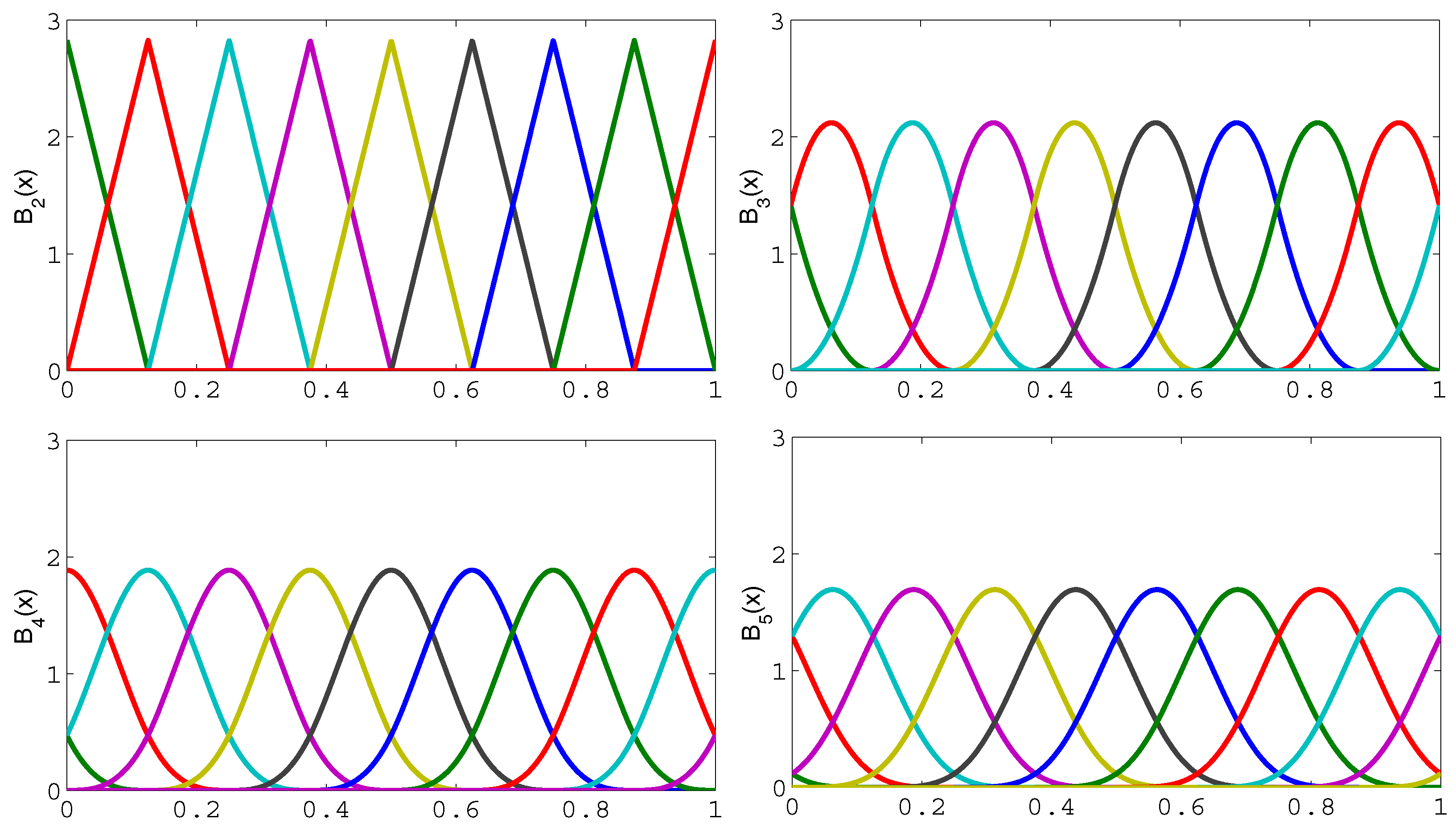
Figure 5.
The estimations of time-varying kernels from an 8-input 1-output system using the dMGLV and the proposed sMGLV modeling methods, where the true kernels are given at 400 s and 800 s, respectively, in two stages. (a) comparing estimation results for different kernels using the dMGLV model and sMGLV model in the first half of the time course; (b) comparing estimation results for different kernels using the dMGLV model and sMGLV model in the second half of the time course
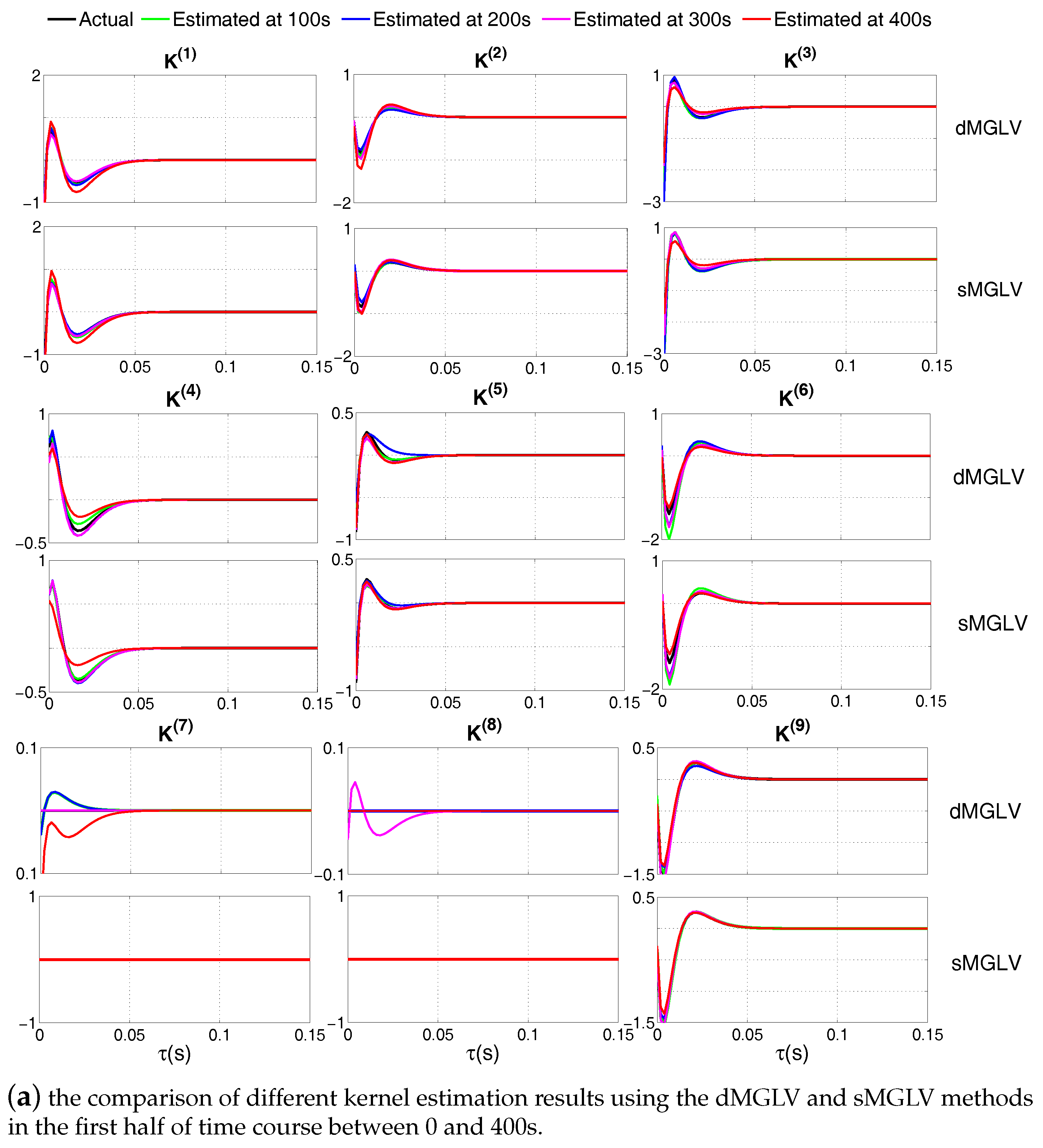

Figure 6.
Kernel shapes for a first-order, 8-input, single-output system with step and linear changes using four different algorithms across simulation time evolution in 2D. The feedback kernel considered in the system can be written as . The amplitudes of the kernels are color-coded.
Figure 6.
Kernel shapes for a first-order, 8-input, single-output system with step and linear changes using four different algorithms across simulation time evolution in 2D. The feedback kernel considered in the system can be written as . The amplitudes of the kernels are color-coded.
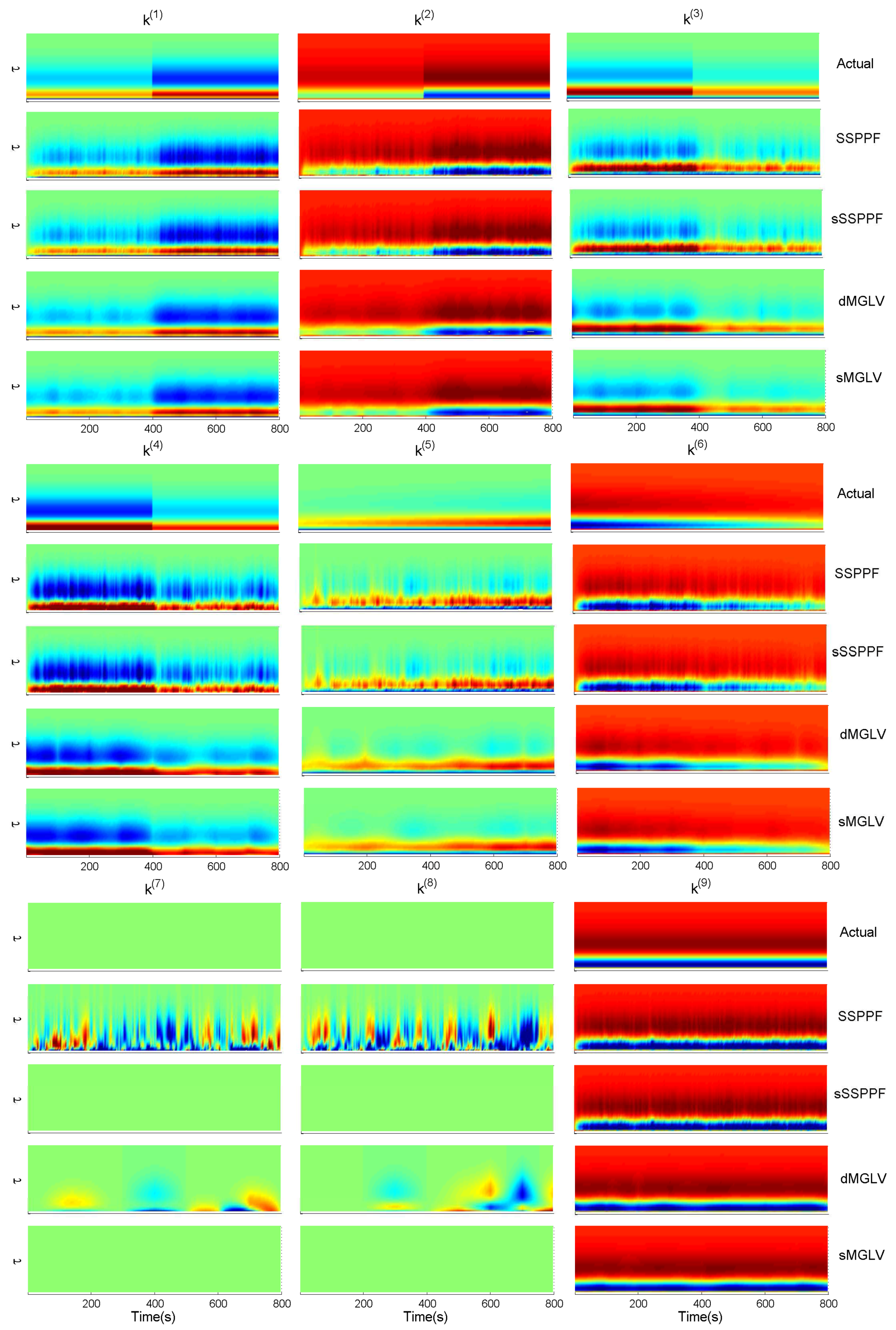
Figure 7.
Peak amplitudes of actual kernels (black) and estimated kernels (blue for SSPPF, green for sSSPPF, purple for dMGLV, and red for the proposed sMGLV model) across simulation time evolution in a time-varying system with a 1 s resolution.
Figure 7.
Peak amplitudes of actual kernels (black) and estimated kernels (blue for SSPPF, green for sSSPPF, purple for dMGLV, and red for the proposed sMGLV model) across simulation time evolution in a time-varying system with a 1 s resolution.
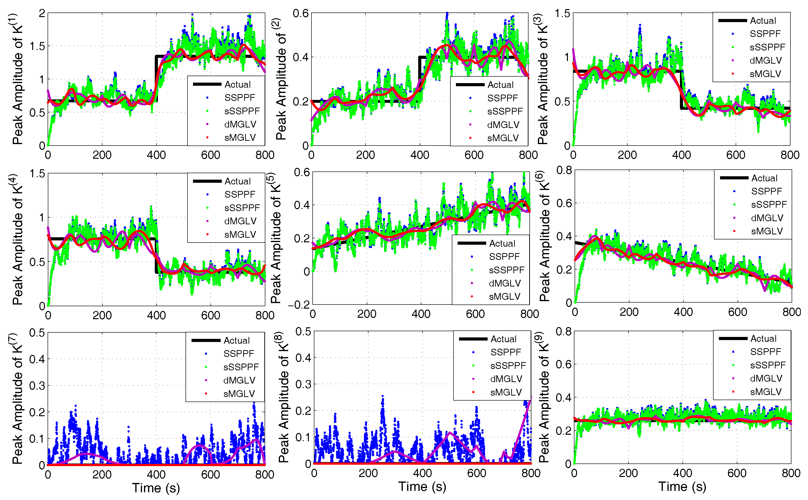
Figure 8.
Estimated output spike train and correlation plot. (a) Estimated output spike train calculated using the proposed sMGLV model. The first row is the estimated firing probability intensity; the second row is the estimated output spike train; the third row is the corresponding actual spike train fragment. (b) Correlation plot. The correlation coefficient r for the whole simulation data length is calculated as a function of the standard deviation of the Gaussian smoothing kernel.

Figure 9.
The estimations of a 4-input and 1-output retina model using the proposed sMGLV modelling method. Estimated kernels using the sMGLV model at different times are drawn with different colors in the left figure; amplitudes and the corresponding stand errors for the estimated kernels can be seen in the right figure.


Table 1.
Table of notations.
| Symbols | Meanings |
|---|---|
| y | Output signal |
| X | Equivalent input signals set |
| M | Memory length of signals |
| Link function of the model | |
| Zeroth-order kernel function | |
| First-order kernel function of the n-th input at lag | |
| Time-Varying Laguerre expansion coefficient of the l-th basis function of the n-th kernel | |
| The l-th order Laguerre basis function | |
| L | Number of Laguerre basis functions |
| Laguerre parameter | |
| P | Composite penalty function |
| Regularization parameter | |
| Time-invariant multiwavelet expansion coefficients | |
| The m-th order Bspline basis function | |
| j | The scale parameter of Bspline basis function |
| m | The order parameter of Bspline basis function |
| p | The number of selected significant model terms |
Table 2.
A performance comparison of kernel estimates for the simulation examples using different approaches.
Table 2.
A performance comparison of kernel estimates for the simulation examples using different approaches.
| Performance Indicators | Estimated Kernels | Identification Methods | |||
|---|---|---|---|---|---|
| SSPPF | sSSPPF | dMGLV | sMGLV | ||
| MSE | 0.1409 | 0.1310 | 0.0592 | 0.0536 | |
| 0.0453 | 0.0435 | 0.0330 | 0.0259 | ||
| 0.0980 | 0.0922 | 0.0483 | 0.0416 | ||
| 0.0911 | 0.0882 | 0.0521 | 0.0408 | ||
| 0.0525 | 0.0529 | 0.0260 | 0.0217 | ||
| 0.0405 | 0.0387 | 0.0222 | 0.0162 | ||
| 0.0431 | 0.0000 | 0.0250 | 0.0000 | ||
| 0.0467 | 0.0000 | 0.0371 | 0.0000 | ||
| 0.0317 | 0.0288 | 0.0078 | 0.0078 | ||
| NRMSE | 0.1987 | 0.1894 | 0.0847 | 0.0791 | |
| 0.2315 | 0.2243 | 0.1472 | 0.1187 | ||
| 0.2337 | 0.2177 | 0.1101 | 0.0991 | ||
| 0.2307 | 0.2229 | 0.1212 | 0.0952 | ||
| 0.2848 | 0.2821 | 0.1270 | 0.1137 | ||
| 0.2370 | 0.2316 | 0.1284 | 0.0875 | ||
| * | - | - | - | - | |
| * | - | - | - | - | |
| 0.1634 | 0.1533 | 0.0425 | 0.0384 | ||
* The NRMSE does not exist considering that the actual kernel values are designed to be zeros.
© 2017 by the authors. Licensee MDPI, Basel, Switzerland. This article is an open access article distributed under the terms and conditions of the Creative Commons Attribution (CC BY) license (http://creativecommons.org/licenses/by/4.0/).
Share and Cite
MDPI and ACS Style
Xu, S.; Li, Y.; Huang, T.; Chan, R.H.M. A Sparse Multiwavelet-Based Generalized Laguerre–Volterra Model for Identifying Time-Varying Neural Dynamics from Spiking Activities. Entropy 2017, 19, 425. https://doi.org/10.3390/e19080425
AMA Style
Xu S, Li Y, Huang T, Chan RHM. A Sparse Multiwavelet-Based Generalized Laguerre–Volterra Model for Identifying Time-Varying Neural Dynamics from Spiking Activities. Entropy. 2017; 19(8):425. https://doi.org/10.3390/e19080425
Chicago/Turabian StyleXu, Song, Yang Li, Tingwen Huang, and Rosa H. M. Chan. 2017. "A Sparse Multiwavelet-Based Generalized Laguerre–Volterra Model for Identifying Time-Varying Neural Dynamics from Spiking Activities" Entropy 19, no. 8: 425. https://doi.org/10.3390/e19080425
Note that from the first issue of 2016, this journal uses article numbers instead of page numbers. See further details here.