Applications of Information Theory in Solar and Space Physics


1
Applied Physics Laboratory, the Johns Hopkins University, Laurel, MD 20723-6099, USA
2
Andrews University, Berrien Springs, MI 49104, USA
*
Author to whom correspondence should be addressed.
Entropy 2019, 21(2), 140; https://doi.org/10.3390/e21020140
Submission received: 10 December 2018
/
Revised: 18 January 2019
/
Accepted: 20 January 2019
/
Published: 1 February 2019
(This article belongs to the Special Issue The 20th Anniversary of Entropy - Recent Advances in Entropy and Information-Theoretic Concepts and Their Applications)
Abstract
:Characterizing and modeling processes at the sun and space plasma in our solar system are difficult because the underlying physics is often complex, nonlinear, and not well understood. The drivers of a system are often nonlinearly correlated with one another, which makes it a challenge to understand the relative effects caused by each driver. However, entropy-based information theory can be a valuable tool that can be used to determine the information flow among various parameters, causalities, untangle the drivers, and provide observational constraints that can help guide the development of the theories and physics-based models. We review two examples of the applications of the information theoretic tools at the Sun and near-Earth space environment. In the first example, the solar wind drivers of radiation belt electrons are investigated using mutual information (MI), conditional mutual information (CMI), and transfer entropy (TE). As previously reported, radiation belt electron flux (Je) is anticorrelated with solar wind density (nsw) with a lag of 1 day. However, this lag time and anticorrelation can be attributed mainly to the Je(t + 2 days) correlation with solar wind velocity (Vsw)(t) and nsw(t + 1 day) anticorrelation with Vsw(t). Analyses of solar wind driving of the magnetosphere need to consider the large lag times, up to 3 days, in the (Vsw, nsw) anticorrelation. Using CMI to remove the effects of Vsw, the response of Je to nsw is 30% smaller and has a lag time <24 h, suggesting that the loss mechanism due to nsw or solar wind dynamic pressure has to start operating in <24 h. Nonstationarity in the system dynamics is investigated using windowed TE. The triangle distribution in Je(t + 2 days) vs. Vsw(t) can be better understood with TE. In the second example, the previously identified causal parameters of the solar cycle in the Babcock–Leighton type model such as the solar polar field, meridional flow, polar faculae (proxy for polar field), and flux emergence are investigated using TE. The transfer of information from the polar field to the sunspot number (SSN) peaks at lag times of 3–4 years. Both the flux emergence and the meridional flow contribute to the polar field, but at different time scales. The polar fields from at least the last 3 cycles contain information about SSN.
1. Introduction
For many complex systems, modeling can be physically or computationally difficult. The coupled solar wind–magnetosphere system is nonlinear and complex. Successful predictions of phenomena such as magnetic storms or substorms have remained notoriously elusive, despite numerous attempts over several decades. It has been known for over a century that the Sun has cool regions of high magnetic flux density that known as sunspots. The number of sunspots exhibits an 11-year cycle, but predicting the sunspot number (SSN) has been largely unsuccessful. The dynamo that generates the sunspots is complex and nonlinear. There have been significant advances in physics-based modeling of solar, magnetospheric, and ionospheric processes, but the global computations are beyond present and/or near future computational capabilities without appropriate approximations. Empirical models that employ intuition assume a priori a dynamical framework that may or may not apply to the system. Moreover, care must be taken because it may be possible to fit the data by choosing enough free parameters at the expense of losing physical understanding or overfitting.
Dependency is a key discriminating statistic that is commonly used to understand how systems operate. The standard tool used to identify dependency is cross-correlation. Considering two variables, x and y, the correlation analysis essentially tries to fit the data to a 2D Gaussian cloud, where the nature of the correlation is determined by the slope and the strength of correlation is determined by the width of the cloud perpendicular to the slope. The correlational analyses are useful, fast, and simple. However, they cannot describe nonlinear relationships and usually cannot be used to establish causalities.
The entropy-based information theory can help identify nonlinearities in the system, information transfer between input and output parameters, and the lag response times. This nonparametric, statistics-based method is not constrained by the assumption of an underlying dynamics---rather the underlying (physics-based) dynamics is discovered by the approach and then ultimately utilized to improve predictions. Moreover, it can help untangle the input parameters that are correlated or anti-correlated with each other. It can also help modelers select input parameters and determine prediction horizon. The latter refers to how far ahead can one predict a variable. Hence, it can be a useful tool to study many complex systems. This approach should be considered complimentary to correlational analyses and to physics-based and empirical modeling approaches.
2. Data Set
The solar wind–radiation belt system study uses daily averages of MeV electron fluxes obtained from Energetic Sensor for Particles (ESP) [5] and Synchronous Orbit Particle Analyzer (SOPA) [6] on board of all seven Los Alamos National Laboratory (LANL) geosynchronous satellites from 22 Sep 1989 to 31 Dec 2009. The data and format description can be found at ftp://ftop.agu.org/apend/ja/2010ja015735. We only examine the fluxes of electrons with energy range of 1.8–3.5 MeVs. A detailed description of the dataset and its processing are given in [7]. The daily and hourly averaged solar wind data 1989–2009 come from OMNI dataset provided by NASA (http://omniweb.gsfc.nasa.gov/). The LANL and solar wind data are merged. The LANL dataset has 7187 data points (days of data), out of which, 6438 data points have simultaneous solar wind observations.
The solar dynamo study uses multiple datasets of the Sun and Earth. The SSN record 1749–2016 is provided by Sunspot Index and Long-term Solar Observations (SILSO) website at http://www.sidc.be/silso/datafiles. The meridional flow dataset 1986–2012 is derived from Mount Wilson Observatory (MWO) dopplergrams and magnetograms as described in [8] and is available at http://www.astro.ucla.edu/~ulrich/. The polar faculae dataset 1906–2014 is based on the consolidated data from MWO, Wilcox Solar Observatory (WSO), and Solar and Heliospheric Observatory (SOHO) Michelson Doppler Imager (MDI) [9]. This dataset is available from Solar Polar Fields Dataverse at https://dataverse.harvard.edu/dataverse/solardynamo. The polar field dataset 1967–2015 is derived from MWO and WSO photospheric field maps with the line of sight profile saturation corrections [10,11] (acquired from Yi-Ming Wang). The record of the aa index (1868–2010) is provided by the National Oceanic and Atmospheric Administration National Centers for Environmental Information (NOAA NCEI) website: ftp://ftp.ngdc.noaa.gov/STP/GEOMAGNETIC_DATA/ and 1869–2015 from International Service of Geomangetic Indices (ISGI) at http://sgi.unistra.fr/indices_aa.php. aa index is a geomagnetic activity index [12]. All the data analysis is performed at monthly resolution.
3. Mutual Information, Conditional Mutual Information, and Transfer Entropy
Information theory has been applied to problems in magnetospheric, ionospheric, and solar physics [13,14,15,16,17,18,19,20,21,22,23,24,25,26]. For example, mutual information and transfer entropy have been successfully used to examine the causal relationships among solar wind, storms, and substorms in the Earth’s magnetosphere [27,28]. Mutual information, conditional mutual information, and transfer entropy are briefly described below, but they are reviewed in [17].
Mutual information (MI) [1,2,29] between two variables, x and y, compares the uncertainty of measuring variables jointly with the uncertainty of measuring the two variables independently. The uncertainty is measured by Shannon entropy. In order to construct the entropies, it is necessary to obtain the probability distribution functions, which in this study are obtained from histograms of the data based on discretization of the variables (i.e., bins). Suppose that two variables, x and y, are binned so that they take on discrete values, and , where
The variables may be thought of as letters in alphabets ℵ1 and ℵ2, which have n and m letters, respectively. The extracted data can be considered as sequences of letters. The entropy associated with each of the variables is defined as
where p() is the probability of finding the letter in the set of x-data and p() is the probability of finding letter in the set of y-data. To examine the relationship between the variables, we extract the word combinations (, from the dataset. The joint entropy is defined by
where is the probability of finding the word combination in the set of (x, y) data. The mutual information [1,2,29] is then defined as
MI (x, y) = H (x) + H (y) − H (x, y)
While MI is useful to identify nonlinear dependence between two variables, it is often useful to consider conditional dependency with respect to a conditioner variable z that takes on discrete values, ∈ { z1, z2, …zn} ℵ3. The conditional mutual information [3]
determines the mutual information between x and y given that z is known. In the case where z is unrelated, CMI(x,y|z) = MI(x,y), but in the case that x or y is known based on z, then CMI(x,y|z) = 0. CMI therefore provides a way to determine how much additional information is known given another variable. CMI can be seen as a special case of the more general conditional redundancy that allows the variable z to be a vector [30].
A common method to establish causal relationships between two time series, e.g., [xt] and [yt], is to use a time-shifted correlation function
where r = correlation coefficient and τ = lag time. The results of this type of analysis may not be particularly clear when the correlation function has multiple peaks or there is not an obvious asymmetry. Additionally, correlational analysis only detects linear correlations. If the feedback involves nonlinear processes, its usefulness may be seriously limited.
Alternatively, time shifted mutual information, MI(x(t), y(t + τ)), can be used to detect causality in nonlinear systems, but this too suffers from the same problems as time-shifted correlation when it has multiple peaks and long range correlations.
A better choice for studying causality is the one-sided transfer entropy [4]
where , k + 1 = dimensionality of the system, and Δ= first minimum in MI[y(t), y(t − τ)]. Transfer entropy (TE) can be considered as a specialized case of conditional mutual information:
where . The transfer entropy can be considered as a conditional mutual information that detects how much average information is contained in an input, x, about the next state of the system, y, that is not contained in the past history, yp, of the system [31]. In the absence of information flow from x to y, TE(x → y) vanishes. Also, unlike correlational analysis and mutual information, transfer entropy is directional, TE(x → y) ≠ TE(y → x). The transfer entropy accounts for static internal correlations, which can be used to determine whether x and y are driven by a common driver or whether x drives y or y drives x.
4. The Solar Wind–Radiation Belt System
The Earth’s radiation belts refer to a region in space that is populated by trapped energetic particles, electrons and ions. Typically, there are two radiation belts: inner belt and outer belt, but sometimes a third belt appears between the two belts [32]. The inner belt is located at equatorial distance approximately between 1.2 and 3 RE (RE = radius of the Earth ~6371 km) from the center of the Earth and is populated by electrons having energies of hundreds of keVs and ions having hundreds of MeVs. The outer belt is located at equatorial distance approximately between 4 and 8 RE and is mostly populated by electrons having energies ranging from a few hundred keVs to tens of MeVs. The present paper deals only with the outer radiation belt electron population.
These radiation belt electrons are often referred to as “killer electrons” because they can cause serious damage to satellites. For example, the radiation belt electrons with energies of a few MeVs or higher can penetrate deep into spacecraft components, while those with energies lower than one MeV can lodge on the surface of the spacecraft bodies, leading to devastating electrical discharges. Radiation belts are quite relevant to the studies of space weather.
The existence of radiation belt MeV electrons is usually explained by some acceleration mechanisms that can accelerate electrons from a few keVs to tens of MeVs. There have been several acceleration mechanisms proposed, but most studies generally suggest either local or global acceleration. In the local acceleration, the storm and substorm injects plasma sheet plasma into the inner-magnetosphere and accelerates low energy (e.g., a few keV) electrons to a few hundred keVs. Once in the inner-magnetosphere, electrons interact with locally grown ultra low frequency (ULF) waves [33,34,35,36,37,38], very low frequency (VLF) waves [39,40,41,42,43], or magnetosonic waves [44,45], which can energize electrons to MeV energy range. Solar wind velocity (Vsw) may be tied to the local acceleration mechanism through substorm particle injections [46,47,48,49,50].
The global acceleration mechanism also invokes ULF waves for electron acceleration, but here the ULF waves are generated globally by Kelvin-Helmholtz instability (KHI) along the magnetopause flanks due to large velocity shear between solar wind and the magnetospheric plasma [51,52,53]. Indeed, studies have shown that Vsw is a dominant, if not the most dominant, driver of relativistic electron fluxes at geosynchronous orbit (6.6 RE) [7,49,54,55,56,57,58].
Figure 1 plots the geosynchronous radiation belt MeV electron flux (Je) vs. Vsw where Je is the relativisic electron flux. The figure shows log Je(t + τ) vs. Vsw(t) for τ = 0, 1, 2, and 7 days. A few things are worth noting. First, the solar wind–radiation belt system is nonlinear and hence the standard linear correlational analysis would be inadequate. Second, the scatter plots in panel a–c look like a triangle, which is discussed in Section 4.2 using information theory. Third, the radiation belt Je is correlated with Vsw. The best correlation can be found with Je with a two-day lag, but it is hard to see this in the scatter plot in Figure 1.
In order to see the best response lag time of the radiation belt Je to Vsw, Figure 2a shows the plot of the corr(Je(t + τ), Vsw(t)). Note that herein, unless otherwise stated, all linear and nonlinear analyses performed with Je uses log Je values. The figure shows that the correlation coefficient peaks at τ = 2 day with r = 0.63. There is a smaller peak at τ = 29 days (r = 0.42), which can be attributed to the 27-day synodic solar rotation. Because the large number of data points (n > 5772), the two peak correlation coefficients are highly significant with p < 0.01 (the probability of two random variables giving a correlation coefficient as large as r is <0.01). However, the linear correlational analysis may be inadequate because the solar wind–radiation belt system is nonlinear (Figure 1). Hence, mutual information and transfer entropy need to be calculated. Figure 2b shows MI(Je(t + τ), Vsw(t)) and TE(Vsw → Je). The figure shows that information transfer from Vsw to Je peaks at τ = 2 days. Although in this case, the linear correlation, MI, and TE peak at the same τ, in general this is not always the case (as shown in the solar cycle analysis in Section 5).
In order to get a measure of the significance of TE(Vsw → Je), we calculate noise = TE[sur(Vsw) → Je] where sur(Vsw) is the surrogate data of Vsw, which is obtained by randomly permuting the order of the time series array Vsw. The mean and standard deviation of the noise are calculated from an ensemble of 100 random permutations of TE[sur(Vsw) → Je]. The mean noise and 3σ (standard deviation) from the mean noise are plotted with solid and dashed green curves, respectively, in Figure 2b. TE(Vsw → Je) peaks at τmax = 2 days where the peak information transfer (itmax) = 0.30, signal to noise ratio (snr) = 5.7 and significance = 94σ where itmax = peak–mean noise, snr = peak/mean noise and significance = itmax/σ(noise). From the snr, itmax, and significance, we conclude that there is a significant transfer of information from Vsw to Je with a 2-day delay. Note that the linear correlation, MI, and TE analyses are consistent with the previous studies [55,56,57,58,59,60,61].
In contrast to Vsw, which correlates with Je, solar wind density (nsw) anticorrelates with Je for reasons that are not entirely clear [49,61]. An increase in nsw would increase solar wind dynamic pressure (Pdyn), which, in turn, would push the magnetopause inward, leading to electron losses at the high L shell [56]. Furthermore, the magnetopause compression would drive ULF waves [62,63,64] leading to fast radial diffusion, which redistributes the losses to lower L shells, including at geosynchronous orbit [49,65,66]. Ukhorskiy et al. [67] used a test particle simulation to demonstrate this scenario, which is known as magnetopause shadowing.
Figure 2c shows that the anticorrelation between nsw and Je minimizes at τ = 1 day (r = −0.49). Figure 2d shows that MI(Je, nsw) and TE(nsw → Je) peak also at τ = 1 day (itmax = 0.13, snr = 4.4 and significance = 42σ). This result is consistent with [60], which finds that Je has the strongest dependence on nsw with a lag of 1 day.
However, Vsw and nsw anti-correlate with each other [68]. Figure 2e shows that the anticorrelation between Vsw and nsw minimizes at τ = 1 day (r = −0.56). Figure 2f shows that MI(nsw(t + τ), Vsw(t)) and TE(Vsw → nsw) peak also at τ = 1 day (itmax = 0.20, snr = 7.4 and significance = 95σ). There is a smaller peak at τ = 28 days, which can be attributed to the 27 day synodic solar rotation.
The anticorrelation of Vsw and nsw with a lag of 1 day complicates the interpretation of the driving of the Je. If Vsw is causally correlated with Je with a lag of 2 days, the anticorrelation between Je and nsw with a lag of 1 day could simply just be coincidence. Conversely, if nsw is causally anticorrelated with Je with a lag of 1 day, the correlation between Vsw and Je could simply just be coincidence. On the other hand, from Figure 2, we cannot rule out the possibility that both Vsw and nsw can exert influence on the Je. If that is the case, how can we untangle the effects of Vsw from nsw and which of these two parameters exert more influence on Je?
4.1. Untangling the Drivers of the Radiation Belt Je
In an attempt to address the above questions, we use conditional mutual information, CMI, to untangle the effects of Vsw from nsw and vice versa. To calculate how much information flows from nsw to Je, given Vsw, we calculate CMI[Je(t + τ), nsw(t)|Vsw(t)], which is plotted as blue curve in Figure 3a. Using a similar approach as for TE, we determine the noise level of the surrogates: CMI[Je(t + τ), sur[nsw(t)] | Vsw(t)]. The mean and σ of the noise are calculated in the same manner as TE and used to determine the significance of the results. The mean noise and 3σ are plotted as solid and dashed green curves respectively. Figure 3a shows that CMI[Je(t + τ), nsw(t) | Vsw(t)] peaks at τmax = 0 day with itmax = 0.091 and snr = 3.2. The τmax = 0 day suggests that Je response lag time to nsw is less than 24 h. However, Figure 3a shows that the peak is rather broad, suggesting that the Je response is still significant at τ = 1 day.
Earlier, we establish that Je(t + 2 days) correlates with Vsw(t), Je(t + 1 day) anticorrelates with nsw(t), but nsw(t + 1 day) anticorrelates with Vsw(t) (Figure 2). In Figure 2d, some of the information in the MI(Je(t + τ), nsw(t)) at τ = 1–2 days actually come from Vsw. MI(Je(t + τ), Vsw(t)) peaks at τ = 2–3 days. Because Vsw anticorrelates with nsw at τ = 1 day, the information in MI(Je(t + τ), Vsw(t)) at τ = 2–3 days would appear in MI(Je(t + τ), nsw(t)) at τ = 1–2 days. Subtracting this information from MI(Je(t + τ), nsw(t)) at τ = 1–2 days would allow the MI(Je(t + τ), nsw(t)) at τ = 0 to become the tallest peak, as shown in Figure 3a. MI(Je(t + τ), nsw(t)) has itmax = 0.21, but removing the effects of Vsw, the itmax drops ~57% to 0.091 (itmax of (CMI[Je(t + 0 day), nsw(t)| Vsw(t)] is 0.091).
Conversely, some of the effects attributed to Vsw can be attributed to nsw, but the effect of nsw is smaller. To see this, we calculate CMI[Je(t + τ), Vsw(t)|nsw(t)], which is plotted in Figure 3b as solid blue curve. The blue curve peaks at τ = 2 days with itmax = 0.25 which is about 2.7 times larger than the itmax of 0.091 for CMI[Je(t + τ), nsw(t)| Vsw(t)]. Thus, Vsw transfers more information to Je than nsw does. MI(Je(t + τ), Vsw(t)) has itmax = 0.32, but removing the effects of nsw, the itmax drops only ~22% to 0.25 (itmax of CMI[Je(t + 2 days), Vsw(t)| nsw(t)] = 0.25).
The reason for the broader peak in Figure 3b is that there is a significant information transfer from nsw to Je at τ = 0–1 day, but it falls off rapidly at larger τ. Because the anticorrelation between Vsw and nsw has a one day lag, removing the effects of nsw would lower MI(Je(t + τ), Vsw(t)) at τ = 1–2 days. So, it for MI(Je(t + τ), Vsw(t)) at τ = 1, 2, and 3 are 0.25, 0.32, and 0.23, respectively, whereas the corresponding values for CMI[Je(t + τ), Vsw(t)| nsw(t)] are 0.14, 0.25, and 0.24, respectively. Note that, at τ = 1 and 2 there are reductions in information while at τ = 3, the information is more or less the same (the difference is within one σ [~0.01]), leading to a broader peak in the CMI[Je(t + τ), Vsw(t)| nsw(t)] curve in Figure 3b than that in the MI(Je, Vsw) curve in Figure 2d.
The above analysis suggests that Vsw is the major driver of Je and shows the Je response time lag to Vsw and nsw. The process to accelerate the electrons to MeV energy range takes 2–3 days, as previously suggested [7,49]. Moreover, based on information transfer from nsw to Je, any mechanism for nsw anticorrelation with Je has to operate or start operating within 24 hr.
Next, we investigate whether other solar wind parameters also contribute to Je. We calculate the information transfer from southward Interplanetary Magnetic Field (IMF) Bz, northward IMF Bz, IMF By, IMF Bx, |IMF B|, Pdyn, σ(IMF B), and solar wind electric field (Esw) to Je, given Vsw. The northward (southward) IMF Bz is calculated from the daily average of the hourly IMF Bz when IMF Bz > 0 (IMF Bz < 0). The results are tabulated in Table 1, which ranks various solar wind parameters based on the itmax. Thus, the ranking gives the importance of each solar wind parameter based on the information transfer to Je. Table 1 also lists τmax which signifies the lag time when information transfer to Je maximizes.
Note that the ranking in Table 1 is obtained with daily resolution data. It is possible that the ranking of some parameters may change if the data are analyzed at higher time resolution. For example, some studies showed that southward IMF Bz can influence Je [69,70,71] but southward IMF Bz is only ranked number 5 in Table 1. IMF fluctuates with periods of northward and southward IMF at minutes or tens of minutes timescale. Thus, the low ranking of the southward IMF Bz most likely result from the fluctuations of IMF Bz within one day period [7,56,60]. Consistent with our result, Li et al. [56] found IMF Bz is poorly correlated with Je at daily resolution.
In Figure 3b, the CMI[Je(t + τ), Vsw(t)| nsw(t)] curve shows that Vsw has little influence on the geosynchronous MeV electrons after a delay of 7–10 days. Thus, using Vsw, the prediction or information horizon for Je is about 7–10 days. Figure 3a shows that using nsw, the prediction horizon for Je is about 2 days.
In applying our information theoretical tools, the number of bins (nb) need to be chosen appropriately. Sturges [72] proposes that for a normal distribution, optimal nb = log2(n) + 1 and bin width (w) = range/nb, where n = number of points in the dataset, range = maximum value–minimum value of the points. In practice, there is usually a range of nb that would work. Using Sturges [72] formula, with roughly 6400 points, nb ~13.6. For the present study, we find that nb = 10 to 15 would work well. Having too few bins would lump too many points into the same bin, leading to loss of information. Conversely, having too many bins would leave many bins with 0 or a low number of points, which also leads to loss of information. For the present study, we choose nb = 10.
4.2. The Triangle Distribution
Reeves et al. [7] was the first to note the right triangle distribution exhibited in Figure 1 panels a–c (the contours in Figure 1d qualitatively look more like parallelograms than right triangles). The left-hand side of the triangle forms because Vsw rarely goes below 300 km s−1. The hypotenuse of the triangle suggests that the lower limit of Je more or less increases with Vsw. The top side of the triangle suggests that Je saturates, which can be attributed to local instabilities [73]. As noted by Reeves et al. [7], the most interesting and perhaps mystifying aspect of the triangle distribution is that high Je is observed for all Vsw conditions and the variability of Je at lower Vsw is much larger than that at higher Vsw.
We investigate the effect of nsw on the triangle distribution. We obtain nsw(t) for each point in the log Je(t + 2 days) vs. Vsw(t) scatter plot in Figure 1c. The nsw in the figure are then binned in 0.3 counts (cm2 s se keV)−1 × 30 km s−1 bins. Figure 4a shows the mean nsw of each bin. Bins with fewer than 15 points are not displayed. The most prominent trend in Figure 4a is a strong density gradient in the x direction because nsw anticorrelates with Vsw.
However, our analysis and Figure 3a suggest that the maximum transfer of information from nsw(t) to Je(t + τ) occurs at τ = 0 day (<24 hr). Hence, instead of assigning nsw(t) to each point in the Je(t + 2 days) vs. Vsw(t) plot, we assign nsw(t + 2 days) so that Je is not time shifted with respect to nsw. We repeat the same procedure done for Figure 4a and the result is shown in Figure 4b. Now, there are density gradients in both x and y directions. As in Figure 4a, the density gradient in the x direction is due to the anticorrelation of nsw with Vsw. Figure 4b clearly shows that for Vsw < 500 km s−1, larger nsw hence larger Pdyn can be associated with lower Je and vice versa. This density gradient in the y direction may be attributed to the magnetopause shadowing effect, which rapidly depletes radiation belt fluxes when solar wind pressure is increases. Thus, the triangle distribution can be explained by the correlation of Vsw(t) and Je(t + 2 days) and the anticorrelation of nsw(t) and Je(t + 0 day).
5. The Solar Cycle
The surface of the Sun has dark regions or spots, commonly called sunspots. The number of sunspots vary cyclically with a period of 11 years, known as solar cycle. Although the cyclical nature of sunspots has been known for over 150 years [74], it is not clear what causes the solar cycle. Predicting SSN remains a challenge [75].
Most solar cycle models today are based on the Babcock–Leighton model [76,77,78]. This is depicted in a diagram in Figure 5 for one hemisphere (see review in [79]). Near the solar minimum, the magnetic field, which has a poloidal configuration, is advected downward to the base of the convection zone, possibly as far down as the tachocline, by the meridional flow from P1 to P2 in Figure 5. From P2, the poloidal field carried by the meridional flow to low latitude (T1). As it does, the latitudinal differential rotation shears the magnetic field, which twists and wraps the field line around the sun azimuthally, leading to the growth of the toroidal field at low latitude at T1. The twisting and turning motions create regions of strong magnetic field, which choke off the plasma and energy flow into the regions and which become buoyant. The buoyancy force pushes these strong magnetic field regions to the surface (photosphere), where they appear at T2. The Coriolis force acting on the rising toroidal field causes the emerging fluxes to appear as pairs of sunspots with a slight tilt such that the following spot of the pair tends to be further from the equator than the preceding spot (Joy’s law), leading to the growth of the poloidal field. As the sunspots decay, the equatorward spot moves equatorward and the poleward spot moves poleward. The equatorward field cancels the one with the opposite polarity from the opposite hemisphere. The meridional flow carries the poleward poloidal field, which has the opposite polarity than that at P1, and which destroys some of the old poloidal fields at P1. This process continues until a new poloidal field with the opposite polarity is established, which commences a new solar cycle. An example of a mathematical formulation of Babcock–Leighton type model can be seen in a flux transport dynamo model [80].
From the description above, it is clear that the meridional flow, which acts as a conveyor belt that circulates the magnetic fluxes, plays an important role in the solar cycle [81,82,83]. Another important parameter is the polar field. Some flux transport dynamo models input the strength of the polar field at solar minimum, which in turn, determines the amplitude of the next solar cycle [82,84,85]. The flux emergence, which can be proxied by SSN, is yet another important parameter as it can affect and be affected by the polar field and meridional flow [82].
The information transfer from the polar field, aa index, polar faculae, and meridional flow to SSN and vice versa are investigated. These parameters are plotted in Figure 6. Because the meridional flow circulates the magnetic fluxes continuously, these parameters, which are magnetic in nature, can affect each other bidirectionally, which poses a challenge. That is, a parameter x can affect y, but y can also affect x some time later. This situation is similar to the well-known predator–prey dynamics [86], where each population affects the other in a causal manner. However, in a situation with multiple species the causal relationship between any two species may have a directionality if one species has a stronger effect on the other species. These bidirectionalities need to be untangled or taken into account with transfer entropy [4].
Our methodology does not a priori assume the relationships between any of the parameters. For example, rather than performing superposed epoch analysis with solar minimum as t = 0, which assumes implicitly or explicitly that solar minimum is the start of the cycle, as done in some studies, we treat the data simply as long time series. In our approach, the solar cycle is a sequence of events (which has occurred for centuries or at least since the data became available) where the meridional flow acting like a perpetual conveyor belt that circulates the magnetic fluxes continuously from the polar region in the photosphere, to low latitude in the convection zone, to the low latitude photosphere, and finally back to the polar region (Figure 5). Therefore, there is no beginning or end to the solar cycle and our results can be viewed as pertaining to the average dynamics of the Sun during the entire period for which the data are analyzed. We are cognizant that the behavior of an individual cycle may vary from one cycle to the next. Hence, care needs to be exercised when using our results to interpret the dynamics of a particular solar cycle. Our approach naturally lends itself to the investigations of the long-term effects (more than a few or several cycles) of one parameter on another, as done in Section 5.4.
5.1. aa Index and SSN
In the study of the Earth’s magnetosphere, it has been known for decades that the amount of active regions at the Sun, proxied by SSN, can cause variations in geomagnetic activity, e.g., the aa index. For example, Coronal Mass Ejections (CMEs) and solar wind high speed streams that occur more frequently during solar maximum and in the declining phase of solar maximum, respectively, can increase the aa index. However, it was suggested that the low level geomagnetic activity is correlated with the strength of interplanetary magnetic field (IMF), which is related to the solar polar field [87,88,89]. In turn, the polar field can affect the sunspot productions sometime later. Ohl [90] and Hathaway et al. [91] showed that the aa index at solar minima is a good predictor of the maximum SSN of the next cycle. Wang and Sheeley [92] reported that when averaged over timescales longer than a month, the aa index is highly correlated with the radial IMF (Br), which is proportional to the Sun’s total open flux, which in turn, is correlated with the Sun’s dipole field strength. For these reasons, the aa index may contain (albeit indirect) some information about the polar field, which facilitates information flow from the aa index to SSN. This scenario is investigated with information theory.
The time shifted correlation between the aa index and SSN is calculated. corr[aa(t), SSN(t + τ] (blue curve) and corr[SSN(t), aa(t + τ)] (red curve) are plotted in Figure 7a. The red curve shows that aa(t + τ) is correlated with SSN(t) with a peak correlation at τ ~30–40 months [correlation coefficient (r) = 0.43] and is anticorrelated with SSN(t) a half solar cycle later. The peak |r| in both the blue and red curves are significant (p < 0.01). Because both the SSN and aa curves are cyclical and attain approximately the same maximum |r| in Figure 7a, it is virtually impossible to discern from the figure whether the aa index is causally related to the SSN or the other way around.
However, the transfer entropy conveys a totally different picture. The transfer entropy from aa to SSN [TE(aa → SSN)] (blue curve) and from SSN to aa [TE(SSN → aa)] (red curve) is presented in Figure 7b. The figure shows that indeed there is a bidirectional flow of information from the aa index to SSN and vice versa. As would be expected, Figure 7b shows that there is more information transfer from the SSN to aa index than the other way around, which the standard correlational analysis cannot establish (Figure 7a). Although the transfer of information from the SSN to aa index has a peak at τ ~ 30–40 months, it has larger peaks at τ > 70 months.
The aa index carries information about the Earth’s magnetospheric dynamics, e.g., [12,21,22]. However, the aa index also carries some information about its drivers such as the IMF, which is related to the polar field. However, as the blue curve in Figure 7b suggests, only a small amount of information about the polar field is embedded within the aa index. The aa index would not be a good proxy for the polar field.
TE(aa → SSN) has peak information transfer (itmax) = 0.20, signal to noise ratio (snr) = 4.3, and significance = 14σ. The bidirectional flow of information between two solar cycle parameters is typical in solar parameters discussed herein. The aa index–SSN example presented here illustrates the power of our methodology.
5.2. Polar Field and SSN
The same analysis done in Section 5.1 is repeated with the polar field and SSN data 1967–2014. corr[polar field(t), SSN(t + τ) (blue curve) and corr[SSN(t), polar field(t + τ)] (red curve) are presented in Figure 8a. The correlation coefficients for both curves peak at τ ~60–70 months (half solar cycle period). This result may be consistent with the Babcock–Leighton model in which the polar field at solar minimum determines the SSN at the next maximum. However, Figure 8b shows that TE(polar field → SSN) peaks at τ ~30–40 months (blue curve). Note that TE(polar field → SSN) calculates the information transfer from the polar field to SSN, given that the present and past values of the SSN are known, which differs from the linear correlation (Figure 8a). The lag time of ~30–40 months is interesting because some models have assumed a lag time of half solar cycle period (66 months). The secondary peak at τ ~0–2 months results from the anticorrelation of the polar field with the SSN with little or no lag.
The lag times of 30–40 months seen in the blue curve in Figure 8b may be related to the time that it takes for the polar field to advect downward and equatorward in the convection zone and to reemerge at the low latitude photosphere. In some models, this time is assumed to be a half the solar cycle period, but our result shows that it can be shorter. This result suggests that perhaps some of the fluxes may emerge at a higher latitude in the equatorial region or some fluxes may submerge at a lower latitude in the polar region. The shorter lag may be consistent with the observations that sunspots of the new cycle appear years before the solar maximum [93,94] and flux emergence at high latitudes [95]. Further investigation is needed.
Figure 8b shows that there is also a significant information transfer from the SSN to the polar field. In fact, there is more information transfer from the SSN to polar field than the other way around. The information transfer from the SSN to polar field has a broad peak at τ ~30–60 months and two narrower peaks at τ ~80–90 months and at τ ~120–130 months. The latter (peak at τ ~120–130 months) may be due to the correlation at the ~11-year solar cycle. Upton and Hathaway [82] suggested that the amount of flux emergence (proxied by the SSN) determines the polar field strength at the next solar minimum. This may be consistent with our result (red curve), but our result shows the maximum response lag times for this process.
The multiple peaks in the red curve in Figure 8b could result from the episodic nature of flux transport to the poles. It is well known that flux is transported to the poles in ‘surge’ with their number and intensity determined by the meridional flow speed [81]. The flux surges take about 2–3 years to reach the poles and seem to last for about 5 years in the period examined, 1967–2014.
All the peaks in the blue and red curves are well above the 3σ from the mean noise (the dashed green line). TE(polar field → SSN) has peak information transfer (itmax) = 0.28, signal to noise ratio (snr) = 5.0, and significance = 19σ.
5.3. The Parameters That Control the Polar Field
It is not clear which parameters play the most dominant role in controlling the polar field. In some surface flux transport models [81,92,96,97,98] a larger meridional flow would lead to weaker polar field and a long cycle whereas in some flux transport dynamo models, it would lead to stronger polar field and a short cycle [84,99]. However, recent studies suggested that the polar field in cycle 23/24 may have been determined to a large extent by the flux emergence, e.g., SSN [82].
Figure 9 presents TE(meridional flow → polar field) (blue curve) and TE(SSN → polar field) (red curve). The plot of TE(SSN → polar field) for 1967–2014 has already been shown in Figure 8b. However, in order to compare it with the meridional flow speed, it is necessary to analyze the data for the same interval when there are the meridional flow data, namely 1986–2012.
It turns out that there is information flow from both the meridional flow and SSN to the polar field, but their relative contribution to the polar field differs at different lag times, as shown in Figure 9. The information transfer from the meridional flow to the polar field is dominant at τ ~28–30 and τ ~90–110 months (almost one solar cycle period) during 1986–2012. The peak at τ ~28–30 months may be consistent with the flux transport dynamo models referenced above and the Schrijver et al. surface flux transport model [100]. However, the transfer of information from the SSN (proxy for the flux emergence) to the polar field is dominant at τ ~60–80 months (about a half solar cycle period) (smaller τ is obtained for the period 1967–2014), which may be consistent with a newly developed surface flux transport model [82]. Our results provide observational constraints for when the information flow from the meridional flow speed and SSN to the polar field should maximize.
All the peaks in the blue and red curves in Figure 9 are well above the 3σ deviation from the mean noise (the dashed green line). For example, peak of TE(meridional flow → polar field) has itmax = 0.71, snr = 3.6, and significance = 17σ. The peak of TE(SSN → polar field) is lower, but is still significant.
5.4. The Importance of the Polar Fields in Last Few Cycles for Predicting SSN
In Dikpati et al. solar flux transport dynamo model [101], the polar field is advected down to the base of the convection zone where it remains for 17–21 years instead of just half the solar cycle period as it travels to low latitude. This polar field becomes the seed for toroidal field that emerges in the photosphere as sunspots. Hence, Dikpati et al. [101] argued that the polar fields not just from the last cycle, but also from the last 3 cycles should affect the production of sunspots. The importance of the polar fields in the past few cycles is also found in the Charbonneau and Dikpati simulation [102], which shows that the toroidal field (proxy for the SSN) at cycle n has the best correlation with the polar field at cycle n–2. This possibility is investigated with information theory. Because the polar field data are available presently for only 4.5 solar cycles, the long-term effect of the polar field is investigated with the polar faculae instead. Studies suggested that polar faculae are as a good proxy for the polar fields [103,104,105,106]. The polar faculae data are available for almost 10 cycles, 1906–2014, which makes it more suitable for the investigation of long-term effects.
Figure 10 presents TE(polar faculae → SSN) (blue curve) and TE(SSN → polar faculae) (red curve). The figure shows that the transfer of information from the polar faculae to SSN peaks at about τ ~30–40 months, consistent with our analysis using the polar field data with shorter timespans in Section 5.2. Thereafter, the information transfer drops to a lower level, but it persists for at least 400 months, which lends support to the idea that the information about the production of the SSN can be found not just from the polar field from the last cycle, but the polar fields from at least the last 3 cycles. However, this may just simply be a reflection of the fact that the solar magnetic field is recycled from one cycle to the next and magnetic flux conservation. Interestingly, TE(polar faculae → SSN) has minima at τ ~120–140 (roughly one solar cycle period) and at τ ~240–260 (roughly two solar cycle periods).
Figure 10 shows that there is actually more information transfer from the SSN to polar faculae than from the polar faculae to SSN, as found earlier with the polar field data with shorter timespans. The figure shows that the information flow from the SSN to polar faculae does peak at around half solar cycle (~50–70 months), but the curve has also other peaks at longer lag times. However, this longer information horizon could perhaps be expected if there is a long-term effect of the polar fields on SSN because the meridional flow circulates the fluxes with a period of a solar cycle.
The analysis has been extended to τ > 400 months. The result indicates that there is still low level information transfer from the polar faculae to the SSN at τ > 400 months (>3 solar cycle period), but the TE gets noisier as τ gets larger because the polar faculae data only span for about 10 cycles.
All the peaks in the blue and red curves are well above the 3σ from the mean noise (the dashed green line). TE(polar faculae → SSN) has itmax = 0.43, snr = 3.3, and significance = 28σ.
6. Concluding Remarks
In the present paper, we show how information theory can be useful in the studies of solar and space physics. Our methodology can generally be applied to a large number of problems because it does not assume a priori the underlying physics of the system. Our findings of information transfer from one parameter to another and the response lag time can provide insights into the physical relationships between the two parameters and provide constraints to models.
We present examples from two applications, one in solar cycle dynamics and one in radiation belt dynamics, each with its own unique challenge. These two examples are intended to show the breadth of the applications of the methodology.
In the radiation belt study, the challenge is that several solar wind drivers can affect the radiation belt flux, Je, simultaneously. We show how information theory can be useful to untangle the drivers of the solar wind–radiation belt system, identify causal parameters, and the system response lag times to the drivers. One of the conclusions is that the radiation belt electron response lag times to Vsw and nsw are 2 and 0 day, respectively. We show that the nonlinearity and the high variability of Je in the triangle distribution can be better understood if we take these response time lags into account.
The solar cycle study presents a particular challenge not found in the radiation belt study, which is that each parameter can affect one another bidirectionally because the solar magnetic field is largely recycled from one cycle to the next. In order to understand the dynamics, these bidirectionalities need to be considered. The simple correlational analysis would not be able to untangle these bidirectionalities, but transfer entropy proves more useful and provides more insights. For example, although the time shifted correlations between aa index and SSN peak at roughly the same value in both directions, the transfer entropy analysis presents a different picture. More information is transferred from SSN to aa index than the other way around, as would be expected because aa index is a poor proxy of the Sun’s polar field.
Moreover, we show that transfer of information from the polar field to SSN peaks at 30–40 months. Both, the meridional flow and SSN transfer information to the polar field, but each parameter dominates at different time lags. The meridional flow transfers more information to the polar field at τ ~28–30 months and τ ~ 90–110 months, whereas SSN transfers more information at τ ~ 60–80 months. Finally, there seems to be support for the idea that the polar field from the last 3 cycles can affect the production of the sunspots because the meridional flow at the bottom of the convective zone is slower than at the top. Our entropy-based approach can be useful to solar cycle modelers and theorists because (1) it can establish which parameters are causally related to the SSN, (2) it can rank the parameters based on the information transfer to the SSN, and (3) it can provide the SSN’s response lag times to these parameters. All of these can provide observational constraints to solar cycle models.
Supplementary Materials
Supplementary File 1Author Contributions
Conceptualization, S.W. and J.R.J.; methodology, S.W. and J.R.J.; software, S.W. and J.R.J.; validation, S.W. and J.R.J.; formal analysis, S.W. and J.R.J.; investigation, S.W. and J.R.J.; resources, The Johns Hopkins University and Andrews University.; data curation, S.W. and J.R.J.; writing—original draft preparation, S.W.; writing—review and editing, S.W. and J.R.J.; visualization, S.W.; supervision, S.W. and J.R.J.; project administration, S.W. and J.R.J.; funding acquisition, J.R.J. and S.W.
Funding
This research was funded by NASA, grant numbers NNX15AJ01G, NNX16AQ87G, NNH11AR07I, NNX14AM27G, NNH14AY20I, NNX16AC39G; NSF, grant numbers ATM0902730 and AGS-1203299; and DOE contract DE-AC02-09CH11466.
Acknowledgments
We would like to thank the reviewers for helpful comments and suggestions. All the derived data products in this paper are available upon request by email ([email protected]).
Conflicts of Interest
The authors declare no conflict of interest.
References
- Li, W. Mutual Information Functions Versus Correlation Functions. J. Stat. Phys. 1990, 60, 823–837. [Google Scholar] [CrossRef]
- Tsonis, A.A. Probing the linearity and nonlinearity in the transitions of the atmospheric circulation. Nonlinear Process. Geophys. 2001, 8, 341–345. [Google Scholar] [CrossRef]
- Wyner, A.D. A definition of conditional mutual information for arbitrary ensembles. Inf. Control 1978, 38, 51–59. [Google Scholar] [CrossRef]
- Schreiber, T. Measuring Information Transfer. Phys. Rev. Lett. 2000, 85, 461–464. [Google Scholar] [CrossRef] [PubMed]
- Meier, M.M.; Belian, R.D.; Cayton, T.E.; Christensen, R.A.; Garcia, B.; Grace, K.M.; Ingraham, J.C.; Laros, J.G.; Reeves, G.D. The energy spectrometer for particles (ESP): Instrument description and orbital performance. AIP Conf. Proc. 1996, 383, 203–210. [Google Scholar]
- Belian, R.D.; Gisler, G.R.; Cayton, T.; Christensen, R. High-Z energetic particles at geosynchronous orbit during the Great Solar Proton Event Series of October 1989. J. Geophys. Res. 1992, 97, 16897–16906. [Google Scholar] [CrossRef]
- Reeves, G.D.; Morley, S.K.; Friedel, R.H.W.; Henderson, M.G.; Cayton, T.E.; Cunningham, G.; Blake, J.B.; Christensen, R.A.; Thomsen, D. On the relationship between relativistic electron flux and solar wind velocity: Paulikas and Blake revisited. J. Geophys. Res. 2011, 116, A02213. [Google Scholar] [CrossRef]
- Ulrich, R.K. Solar Meridional Circulation from Doppler Shifts of the Fe I Line at 5250 Å as Measured by the 150-foot Solar Tower Telescope at the Mt. Wilson Observatory. Astrophys. J. 2010, 725, 658–669. [Google Scholar] [CrossRef]
- Muñoz-Jaramillo, A.; Sheeley, N.R., Jr.; Zhang, J.; DeLuca, E.E. Calibrating 100 years of polar faculae measurements: Implications for the evolution of the heliospheric magnetic field. Astrophys. J. 2012, 753, 146. [Google Scholar] [CrossRef]
- Ulrich, R.K. Cool Stars, Stellar Systems, and the Sun; Giampapa, M.S., Bookbinder, J.S., Eds.; ASP Conf. Ser.; Astronomical Society of the Pacific: San Francisco, CA, USA, 1992; Volume 26, p. 265. [Google Scholar]
- Wang, Y.-M.; Sheeley, N.R., Jr. Solar Implications of ULYSSES Interplanetary Field Measurements. Astrophys. J. Lett. 1995, 447, L143. [Google Scholar] [CrossRef]
- Mayaud, P.-N. The aa indices: A 100-year series characterizing the magnetic activity. J. Geophys. Res. 1972, 77, 6870–6874. [Google Scholar] [CrossRef]
- Consolini, G.; Tozzi, R.; de Michelis, P. Complexity in the sunspot cycle. A A 2009, 506, 1381–1391. [Google Scholar] [CrossRef]
- Balasis, G.; Daglis, I.A.; Papadimitriou, C.; Kalimeri, M.; Anastasiadis, A.; Eftaxias, K. Dynamical complexity in Dst time series using non-extensive Tsallis entropy. Geophys. Res. Lett. 2008, 35, L14102. [Google Scholar] [CrossRef]
- Balasis, G.; Daglis, I.A.; Papadimitriou, C.; Kalimeri, M.; Anastasiadis, A.; Eftaxias, K. Investigating dynamical complexity in the magnetosphere using various entropy measures. J. Geophys. Res. 2009, 114, A00D06. [Google Scholar] [CrossRef]
- Balasis, G.; Papadimitriou, C.; Daglis, I.A.; Anastasiadis, A.; Athanasopoulou, L.; Eftaxias, K. Signatures of discrete scale invariance in Dst time series. Geophys. Res. Lett. 2011, 38, L13103. [Google Scholar] [CrossRef]
- Balasis, G.; Donner, R.V.; Potirakis, S.M.; Runge, J.; Papadimitriou, C.; Daglis, I.A.; Eftaxias, K.; Kurths, J. Statistical mechanics and information-theoretic perspectives on complexity in the Earth system. Entropy 2013, 15, 4844–4888. [Google Scholar] [CrossRef]
- Materassi, M.; Ciraolo, L.; Consolini, G.; Smith, N. Predictive Space Weather: An information theory approach. Adv. Space Res. 2011, 47, 877–885. [Google Scholar] [CrossRef]
- De Michelis, P.; Tozzi, R.; Consolini, G. Statistical analysis of geomagnetic field intensity differences between ASM and VFM instruments onboard Swarm constellation. Earth Planets Space 2017, 69, 24. [Google Scholar] [CrossRef]
- March, T.K.; Chapman, S.C.; Dendy, R.O. Mutual information between geomagnetic indices and the solar wind as seen by WIND: Implications for propagation time estimates. Geophys. Res. Lett. 2005, 32, L04101. [Google Scholar] [CrossRef]
- Johnson, J.R.; Wing, S. A solar cycle dependence of nonlinearity in magnetospheric activity. J. Geophys. Res. 2005, 110, A04211. [Google Scholar] [CrossRef]
- Wing, S.; Johnson, J.R.; Jen, J.; Meng, C.-I.; Sibeck, D.G.; Bechtold, K.; Freeman, J.; Costello, K.; Balikhin, M.; Takahashi, K. Kp forecast models. J. Geophys. Res. 2005, 110, A04203. [Google Scholar] [CrossRef]
- Wing, S.; Johnson, J.R.; Camporeale, E.; Reeves, G.D. Information theoretical approach to discovering solar wind drivers of the outer radiation belt. J. Geophys. Res. Space Phys. 2016, 121, 9378–9399. [Google Scholar] [CrossRef]
- Johnson, J.R.; Wing, S. External versus internal triggering of substorms: An information-theoretical approach. Geophys. Res. Lett. 2014, 41, 5748–5754. [Google Scholar] [CrossRef]
- Wing, S.; Johnson, J.; Vourlidas, A. Information theoretic approach to discovering causalities in the solar cycle. ApJ 2018, 854, 85. [Google Scholar] [CrossRef]
- Johnson, J.R.; Wing, S.; Camporeale, E. Transfer entropy and cumulant-based cost as measures of nonlinear causal relationships in space plasmas: Applications to Dst. Ann. Geophys. 2018, 36, 945–952. [Google Scholar] [CrossRef]
- De Michelis, P.; Consolini, G.; Materassi, M.; Tozzi, R. An information theory approach to the storm-substorm relationship. J. Geophys. Res. 2011, 116, A08225. [Google Scholar] [CrossRef]
- Runge, J.; Balasis, G.; Daglis, I.A.; Papadimitriou, C.; Donner, R.V. Common solar wind drivers behind magnetic storm–magnetospheric substorm dependency. Sci. Rep. 2018, 8, 16987. [Google Scholar] [CrossRef]
- Darbellay, G.A.; Vajda, I. Estimation of the Information by an Adaptive Partitioning of the Observations Space. IEEE Trans. Inf. Theory 1999, 45, 1315–1321. [Google Scholar] [CrossRef]
- Prichard, D.; Theiler, J. Generalized redundancies for time series analysis. Physica D 1995, 84, 476–493. [Google Scholar] [CrossRef]
- Prokopenko, M.; Lizier, J.T.; Price, D.C. On thermodynamic interpretation of transfer entropy. Entropy 2013, 15, 524–543. [Google Scholar] [CrossRef]
- Baker, D.N.; Kanekal, S.G.; Hoxie, V.C.; Henderson, M.G.; Li, X.; Spence, H.E.; Elkington, S.R.; Friedel, R.H.W.; Goldstein, J.; Hudson, M.K.; et al. A long-lived relativistic electron storage ring embedded in Earth’s outer Van Allen belt. Science 2013, 340, 186–190. [Google Scholar] [CrossRef] [PubMed]
- Elkington, S.R.; Hudson, M.K.; Chan, A.A. Acceleration of relativistic electrons via drift-resonant interaction with toroidal-mode Pc-5 ULF oscillations. Geophys. Res. Lett. 1999, 26, 3273. [Google Scholar] [CrossRef]
- Rostoker, G.; Skone, S.; Baker, D.N. On the origin of relativistic electrons in the magnetosphere associated with some geomagnetic storms. Geophys. Res. Lett. 1998, 25, 3701–3704. [Google Scholar] [CrossRef]
- Ukhorskiy, A.Y.; Takahashi, K.; Anderson, B.J.; Korth, H. Impact of toroidal ULF waves on the outer radiation belt electrons. J. Geophys. Res. 2005, 110, A10202. [Google Scholar] [CrossRef]
- Mathie, R.A.; Mann, I.R. A correlation between extended intervals of ULF wave power and storm-time geosynchronous relativistic electron flux enhancements. Geophys. Res. Lett. 2000, 27, 3261–3264. [Google Scholar] [CrossRef]
- Mathie, R.A.; Mann, I.R. On the solar wind control of Pc5 ULF pulsation power at mid-latitudes: Implications for MeV electron acceleration in the outer radiation belt. J. Geophys. Res. 2001, 106, 29783–29796. [Google Scholar] [CrossRef]
- Georgiou, M.; Daglis, I.A.; Rae, I.J.; Zesta, E.; Sibeck, D.G.; Mann, I.R.; Balasis, G.; Tsinganos, K. Ultra-Low Frequency waves as an interme-diary for solar wind energy input into the radiation belts. J. Geophys. Res. Space Phys. 2018, 123. [Google Scholar] [CrossRef]
- Summers, D.; Thorne, R.M.; Xiao, F. Relativistic theory of wave-particle resonant diffusion with application to electron acceleration in the magnetosphere. J. Geophys. Res. 1998, 103, 20487–20500. [Google Scholar] [CrossRef]
- Omura, Y.; Furuya, N.; Summers, D. Relativistic turning acceleration of resonant electrons by coherent whistler mode waves in a dipole magnetic field. J. Geophys. Res. 2007, 112, A06236. [Google Scholar] [CrossRef]
- Thorne, R.M. Radiation belt dynamics: The importance of wave-particle interactions. Geophys. Res. Lett. 2010, 37, L22107. [Google Scholar] [CrossRef]
- Simms, L.E.; Engebretson, M.J.; Smith, A.J.; Clilverd, M.; Pilipenko, V.; Reeves, G.D. Analysis of the effectiveness of ground-based VLF wave observations for predicting or nowcasting relativistic electron flux at geostationary orbit. J. Geophys. Res. Space Phys. 2015, 120, 2052–2060. [Google Scholar] [CrossRef]
- Camporeale, E. Resonant and nonresonant whistlers-particle interaction in the radiation belts. Geophys. Res. Lett. 2015, 42, 3114–3121. [Google Scholar] [CrossRef]
- Horne, R.B.; Thorne, R.M.; Glauert, S.A.; Meredith, N.P.; Pokhotelov, D.; Santolík, O. Electron acceleration in the Van Allen radiation belts by fast magnetosonic waves. Geophys. Res. Lett. 2007, 34, L17107. [Google Scholar] [CrossRef]
- Shprits, Y.Y.; Subbotin, D.A.; Meredith, N.P.; Elkington, S.R. Review of modeling of losses and sources of relativistic electrons in the outer radiation belt II: Local acceleration and loss. J. Atmos. Sol. Terr. Phys. 2008, 70, 1694–1713. [Google Scholar] [CrossRef]
- Baker, D.N.; Kanekal, S.G. Solar cycle changes, geomagnetic variations, and energetic particle properties in the inner magnetosphere. J. Atmos. Sol. Terr. Phys. 2008, 70, 195–206. [Google Scholar] [CrossRef]
- Kissinger, J.; McPherron, R.L.; Hsu, T.-S.; Angelopoulos, V. Steady magnetospheric convection and stream interfaces: Relationship over a solar cycle. J. Geophys. Res. 2011, 116, A00I19. [Google Scholar] [CrossRef]
- Tanskanen, E.I. A comprehensive high-throughput analysis of substorms observed by IMAGE magnetometer network: Years 1993–2003 examined. J. Geophys. Res. 2009, 114, A05204. [Google Scholar] [CrossRef]
- Kellerman, A.C.; Shprits, Y.Y. On the influence of solar wind conditions on the outer-electron radiation belt. J. Geophys. Res. 2012, 117, A05217. [Google Scholar] [CrossRef]
- Newell, P.T.; Liou, K.; Gjerloev, J.W.; Sotirelis, T.; Wing, S.; Mitchell, E.J. Substorm probabilities are best predicted from solar wind speed. J. Atmos. Sol. Terr. Phys. 2016, 146, 28–37. [Google Scholar] [CrossRef]
- Johnson, J.R.; Wing, S.; Delamere, P.A. Kelvin Helmholtz Instability in Planetary Magnetospheres. Space Sci. Rev. 2014, 184, 1–31. [Google Scholar] [CrossRef]
- Engebretson, M.; Glassmeier, K.-H.; Stellmacher, M.; Hughes, W.J.; Lühr, H. The dependence of high-latitude PcS wave power on solar wind velocity and on the phase of high-speed solar wind streams. J. Geophys. Res. 1998, 103, 26271–26283. [Google Scholar] [CrossRef]
- Vennerstrøm, S. Dayside magnetic ULF power at high latitudes: A possible long-term proxy for the solar wind velocity? J. Geophys. Res. 1999, 104, 10145–10157. [Google Scholar] [CrossRef]
- Paulikas, G.A.; Blake, J.B. Effects of the solar wind on magnetospheric dynamics: Energetic electrons at the synchronous orbit. In Quantitative Modeling of Magnetospheric Processes; Geophysical Monograph Series; AGU: Washington, DC, USA, 1979; Volume 21, pp. 180–202. [Google Scholar]
- Baker, D.N.; McPherron, R.L.; Cayton, T.E.; Klebesadel, R.W. Linear prediction filter analysis of relativistic electron properties at 6.6 RE. J. Geophys. Res. 1990, 95, 15133–15140. [Google Scholar] [CrossRef]
- Li, X.; Temerin, M.; Baker, D.; Reeves, G.; Larson, D. Quantitative prediction of radiation belt electrons at geostationary orbit based on solar wind measurements. Geophys. Res. Lett. 2001, 28, 1887–1890. [Google Scholar] [CrossRef]
- Vassiliadis, D.; Fung, S.F.; Klimas, A.J. Solar, interplanetary, and magnetospheric parameters for the radiation belt energetic electron flux. J. Geophys. Res. 2005, 110, A04201. [Google Scholar] [CrossRef]
- Ukhorskiy, A.Y.; Sitnov, M.I.; Sharma, A.S.; Anderson, B.J.; Ohtani, S.; Lui, A.T.Y. Data-derived forecasting model for relativistic electron intensity at geosynchronous orbit. Geophys. Res. Lett. 2004, 31, L09806. [Google Scholar] [CrossRef]
- Rigler, E.J.; Wiltberger, M.; Baker, D.N. Radiation belt electrons respond to multiple solar wind inputs. J. Geophys. Res. 2007, 112, A06208. [Google Scholar] [CrossRef]
- Balikhin, M.A.; Boynton, R.J.; Walker, S.N.; Borovsky, J.E.; Billings, S.A.; Wei, H.L. Using the NARMAX approach to model the evolution of energetic electrons fluxes at geostationary orbit. Geophys. Res. Lett. 2011, 38, L18105. [Google Scholar] [CrossRef]
- Lyatsky, W.; Khazanov, G.V. Effect of solar wind density on relativistic electrons at geosynchronous orbit. Geophys. Res. Lett. 2008, 35, L03109. [Google Scholar] [CrossRef]
- Korotova, G.I.; Sibeck, D.G. A case study of transient event motion in the magnetosphere and in the ionosphere. J. Geophys. Res. 1995, 100, 35–46. [Google Scholar] [CrossRef]
- Kepko, L.; Spence, H.E. Observations of discrete, global magnetospheric oscillations directly driven by solar wind density variations. J. Geophys. Res. 2003, 108, 1257. [Google Scholar] [CrossRef]
- Claudepierre, S.G.; Hudson, M.K.; Lotko, W.; Lyon, J.G.; Denton, R.E. Solar wind driving of magnetospheric ULF waves: Field line resonances driven by dynamic pressure fluctuations. J. Geophys. Res. 2010, 115, A11202. [Google Scholar] [CrossRef]
- Shprits, Y.Y.; Thorne, R.M.; Friedel, R.; Reeves, G.D.; Fennell, J.; Baker, D.N.; Kanekal, S.G. Outward radial diffusion driven by losses at magnetopause. J. Geophys. Res. 2006, 111, A11214. [Google Scholar] [CrossRef]
- Turner, D.L.; Shprits, Y.; Hartinger, M.; Angelopoulos, V. Explaining sudden losses of outer radiation belt electrons during geomagnetic storms. Nat. Phys. 2012, 8, 208–212. [Google Scholar] [CrossRef]
- Ukhorskiy, A.Y.; Anderson, B.J.; Brandt, P.C.; Tsyganenko, N.A. Storm time evolution of the outer radiation belt: Transport and losses. J. Geophys. Res. 2006, 111, A11S03. [Google Scholar] [CrossRef]
- Hundhausen, A.J.; Bame, S.J.; Asbridge, J.R.; Sydoriak, S.J. Solar wind proton properties: Vela 3 observations from July 1965 to June 1967. J. Geophys. Res. 1970, 75, 4643–4657. [Google Scholar] [CrossRef]
- Li, X.; Baker, D.N.; Temerin, M.; Reeves, G.; Friedel, R.; Shen, C. Energetic electrons, 50 keV to 6 MeV, at geosynchronous orbit: Their responses to solar wind variations. Space Weather 2005, 3, S04001. [Google Scholar] [CrossRef]
- Onsager, T.G.; Green, J.C.; Reeves, G.D.; Singer, H.J. Solar wind and magnetospheric conditions leading to the abrupt loss of outer radiation belt electrons. J. Geophys. Res. 2007, 112, A01202. [Google Scholar] [CrossRef]
- Miyoshi, Y.; Kataoka, R. Flux enhancement of the outer radiation belt electrons after the arrival of stream interaction regions. J. Geophys. Res. 2008, 113, A03S09. [Google Scholar] [CrossRef]
- Sturges, H.A. The choice of a class interval. J. Am. Stat. Assoc. 1926, 21, 65–66. [Google Scholar] [CrossRef]
- Kennel, C.F.; Petschek, H.E. Limit on stably trapped particle fluxes. J. Geophys. Res. 1966, 71, 1–28. [Google Scholar] [CrossRef]
- Schwabe, H. Sonnen-Beobachtungen im Jahre 1843. Astron. Nachr. 1844, 21, 233–235. [Google Scholar] [CrossRef]
- Pesnell, W.D. Predictions of Solar Cycle 24: How are we doing? Space Weather 2016, 14, 10–21. [Google Scholar] [CrossRef]
- Babcock, H.W. The Topology of the Sun’s Magnetic Field and the 22-Year Cycle. Astrophys. J. 1961, 133, 572–589. [Google Scholar] [CrossRef]
- Leighton, R.B. Transport of magnetic fields on the sun. Astrophys. J. 1964, 140, 1547–1562. [Google Scholar] [CrossRef]
- Leighton, R.B. A magneto-kinematic model of the solar cycle. Astrophys. J. 1969, 156, 1–26. [Google Scholar] [CrossRef]
- Charbonneau, P. Dynamo models of the solar cycle. Living Rev. Sol. Phys. 2010, 7, 3. [Google Scholar] [CrossRef]
- Dikpati, M.; Charbonneau, P. A Babcock–Leighton flux transport dynamo with solar-like differential rotation. Astrophys. J. 1999, 518, 508–520. [Google Scholar] [CrossRef]
- Wang, Y.-M.; Nash, A.G.; Sheeley, N.R., Jr. Evolution of the sun’s polar fields during sunspot cycle 21—Poleward surges and long-term behavior. Astrophys. J. 1989, 347, 529–539. [Google Scholar] [CrossRef]
- Upton, L.; Hathaway, D.H. Effects of meridional flow variations on solar cycles 23 and 24. Astrophys. J. 2014, 792, 142. [Google Scholar] [CrossRef]
- Kholikov, S.; Serebryanskiy, A.; Jackiewicz, J. Meridional flow in the solar convection zone. I. Measurements from GONG data. ApJ 2014, 784. [Google Scholar] [CrossRef]
- Choudhuri, A.R.; Chatterjee, P.; Jiang, J. Predicting Solar Cycle 24 With a Solar Dynamo Model. Phys. Rev. Lett. 2007, 98, 131103. [Google Scholar] [CrossRef]
- Schatten, K.H.; Scherrer, P.H.; Svalgaard, L.; Wilcox, J.M. Using dynamo theory to predict the sunspot number during solar cycle 21. Geophys. Res. Lett. 1978, 5, 411–414. [Google Scholar] [CrossRef]
- Hu, F.; Nie, L.-J.; Fu, S.-J. Information dynamics in the interaction between a prey and a predator fish. Entropy 2015, 17, 7230–7241. [Google Scholar] [CrossRef]
- Schatten, K.H.; Sofia, S. Forecast of an exceptionally large even-numbered solar cycle. Geophys. Res. Lett. 1987, 14, 632–635. [Google Scholar] [CrossRef]
- Schatten, K.H.; Pesnell, D. An early solar dynamo prediction: Cycle 23–cycle 22. Geophys. Res. Lett. 1993, 20, 2275–2278. [Google Scholar] [CrossRef]
- Layden, A.C.; Fox, P.A.; Howard, J.M.; Sarajedini, A.; Schatten, K.H.; Sofia, S. Dynamo-based scheme for forecasting the magnitude of solar activity cycles. Sol. Phys. 1991, 132, 1–40. [Google Scholar] [CrossRef]
- Ohl, A.I. Forecast of sunspot maximum number of cycle 20. Byull. Soln. Dannye Akad. Nauk SSSR 1966, 9, 84. [Google Scholar]
- Hathaway, D.H.; Wilson, R.M.; Reichmann, E.J. A synthesis of solar cycle prediction techniques. J. Geophys. Res. 1999, 104. [Google Scholar] [CrossRef]
- Wang, Y.-M.; Sheeley, N.R., Jr. Understanding the geomagnetic precursor of the solar cycle. Astrophys. J. 2009, 694, L11–L15. [Google Scholar] [CrossRef]
- Svalgaard, L.; Cliver, E.W.; Kamide, Y. Sunspot cycle 24: Smallest cycle in 100 years? Geophys. Res. Lett. 2005, 32, L01104. [Google Scholar] [CrossRef]
- Harvey, K.L. Large scale patterns of magnetic activity and the solar cycle. Bull. Am. Astron. Soc. 1996, 28, 867. [Google Scholar]
- Makarov, V.I.; Tlatov, A.G.; Callebaut, D.K.; Obridko, V.N.; Shelting, B.D. Large scale magnetic field and sunspot cycles. Sol. Phys. 2001, 198, 409–421. [Google Scholar] [CrossRef]
- DeVore, C.R.; Sheeley, N.R. Simulations of the sun’s polar magnetic fields during sunspot cycle 21. Sol. Phys. 1987, 108, 47. [Google Scholar] [CrossRef]
- Schrijver, C.J.; Title, A.M. On the Formation of Polar Spots in Sun-like Stars. Astrophys. J. 2001, 551, 1099–1106. [Google Scholar] [CrossRef]
- Wang, Y.-M.; Sheeley, N.R., Jr; Lean, J. Meridional flow and the solar cycle variations of the Sun’s open magnetic flux. Astrophys. J. 2002, 580, 1188–1196. [Google Scholar] [CrossRef]
- Dikpati, M.; de Toma, G.; Gilman, P.A. Predicting the strength of solar cycle 24 using a flux-transport dynamo-based tool. Geophys. Res. Lett. 2006, 33, L05102. [Google Scholar] [CrossRef]
- Schrijver, C.J.; De Rosa, M.L.; Title, A.M. What is missing from our understanding of long term solar and heliospheric activity? Astrophys. J. 2002, 577, 1006–1012. [Google Scholar] [CrossRef]
- Dikpati, M.; de Toma, G.; Gilman, P.A.; Arge, C.N.; White, O.R. Diagnostics of polar field reversal in solar cycle 23 using a flux-transport dynamo model. Astrophys. J. 2004, 601, 1136–1151. [Google Scholar] [CrossRef]
- Charbonneau, P.; Dikpati, M. Stochastic Fluctuations in a Babcock–Leighton Model of the Solar Cycle. Astophys. J. 2000, 543, 1027–1043. [Google Scholar] [CrossRef]
- Sheeley, N.R., Jr. Polar faculae during the sun- spot cycle. Astrophys. J. 1964, 140, 731. [Google Scholar] [CrossRef]
- Sheeley, N.R., Jr. Measurements of solar magnetic fields. Astrophys. J. 1966, 144, 728. [Google Scholar] [CrossRef]
- Sheeley, N.R., Jr. Polar faculae during the interval 1906–1975. J. Geophys. Res. 1976, 81, 3462–3464. [Google Scholar] [CrossRef]
- Sheeley, N.R. Polar faculae. Astrophys. J. 1991, 374, 386–389. [Google Scholar] [CrossRef]
Figure 1.
Scatter plots of log Je(t + τ) vs. Vsw(t) for τ = 0, 1, 2, and 7 days in panels (a), (b), (c), and (d), respectively. The data points are overlain with density contours showing the nonlinear trends. The panels show that Je has dependence on Vsw for τ = 0, 1, and 2 days and the dependence is strongest for τ = 2 days. (d) At large τ, e.g., τ = 7 day, Je dependence on Vsw is very weak. This figure is essentially the same as Figure 9 in [7], except that no density contours are drawn and Figure 1d plots τ = 7 days instead of τ = 3 days. (from [23]).

Figure 2.
(a) Correlation coefficient of [Je(t + τ), Vsw(t)]. (b) MI[Je(t + τ), Vsw(t)] (blue) and TE[Je(t + τ), Vsw(t)] (yellow). The transfer of information from Vsw to Je [TE (Vsw → Je)] peaks at τmax = 2 days. (c) Correlation coefficient of [Je(t + τ), nsw(t)]. (d) MI[Je(t + τ), nsw(t)] (blue) and TE[Je(t + τ), nsw(t)] (yellow). The transfer of information from nsw to Je [TE (nsw → Je)] peaks at τmax = 1 day. (e) Correlation coefficient of [nsw(t + τ), Vsw(t)]. (f) MI[nsw(t + τ), Vsw(t)] (blue) and TE[nsw(t + τ), Vsw(t)] (yellow). The solid and dashed green curves are the mean and 3σ from the mean of the noise. The transfer of information from Vsw to nsw [TE (Vsw → nsw)] peaks at τmax = 1 day. (adapted from [23]).

Figure 3.
Blue curve showing (a) CMI[Je(t + τ), nsw(t) | Vsw(t)], and (b) CMI[Je(t + τ), Vsw(t) | nsw(t)]. The solid and dashed green curves are the mean and 3σ from the mean of the noise. (a) Unlike MI(Je, nsw), which peaks at τmax = 1 day, CMI[Je(t + τ), nsw(t) | Vsw(t)] peaks at τmax = 0 day (itmax = 0.091). The smaller τmax occurs because CMI removes the effect of Vsw on Je (see text). (b) The peak in CMI[Je(t + τ), Vsw(t) | nsw(t)] (itmax = 0.25) is broader than that of MI(Je, Vsw) in Figure 2b because CMI removes the effect of nsw, which anticorrelates with Je. Vsw transfers about 2.7 times more information to Je than nsw. (from [23]).

Figure 4.
Points in Je(t + 2 days) vs. Vsw(t) distribution in Figure 1c are binned in 0.3 counts (cm2 s sr keV)−1 × 30 km s−1 bins. Each point is assigned its nsw(t) and nsw(t + 2 days) values. The latter has no time shift with respect to Je such that information transfer from nsw to Je maximizes. (a) shows the mean nsw(t) while (b) shows the mean nsw(t + 2 days) of each bin. In (a), the density gradient is mainly in the x direction due to the anticorrelation between nsw and Vsw. However, in (b), there are density gradients in x and y direction. The latter can be attributed to Pdyn and magnetopause shadowing. (from [23].)

Figure 5.
Babcock–Leighton type solar cycle dynamo model. The diagram shows a meridional slice of the sun. The meridional flow is plotted in green with arrows indicating the flow direction. Poloidal field at P1 is advected down to P2 in the convective zone by the meridional flow. The meridional flow advects the field from P2 to T1, while the differential rotation shears the field, converting it to toroidal field. The buoyancy force lifts the toroidal field from T1 to the photosphere at T2, producing sunspots. The sunspots decay into poloidal field, which is carried by the meridional flow to the T1 and the cycle starts over again. (from [25]).

Figure 6.
Solar cycle variations of (a) aa index; (b) the solar polar faculae calibrated to SOHO MDI polar magnetic flux [9]; (c) the solar polar field strength; (d) the meridional flow. These parameters are plotted in red curves whereas the SSN is plotted in the blue curves. The SSN has been scaled by a different factor in each figure as indicated by the right y-axis label in order to enhance viewing. (adapted from [25]).

Figure 7.
(a) Time shifted correlation corr[aa index(t), SSN(t + τ)] is plotted in blue and corr[SSN(t), aa index(t + τ)] is plotted in red. The peak |corr[aa index(t), SSN(t + τ)]| is roughly the same as the peak |corr[SSN(t), aa index(t + τ)]|. (b) TE(aa index → SSN) is plotted in blue and TE(SSN → aa index) is plotted in red. TE(SSN → aa index) > TE(aa index → SSN), suggesting that more information is transferred from the SSN to aa index than the other way around. Such information cannot be discerned from the correlations shown in (a). The solid and dashed green curves show the mean and 3σ of the noise (see text). The data are for the period 1967–2014. (from [25]).

Figure 8.
(a) Time shifted correlation corr[polar field(t), SSN(t + τ)] is plotted in blue and corr[SSN(t), polar field(t + τ)] is plotted in red. They both reach minima at τ ~0 month and maxima at τ ~60–70 months (half solar cycle period) because the polar field and SSN tend to be 180° out of phase with each other. (b) TE(polar field → SSN) is plotted in blue and TE(SSN → polar field) is plotted in red. The format is the same as in Figure 7. The transfer of information from the polar field to SSN peaks at τ ~30–40 months. There is significant information transfer from the SSN to polar field as well. The solid and dashed green curves show the mean and 3σ of the noise. The data are for the period 1967–2014. (from [25]).

Figure 9.
TE(meridional flow → polar field) and TE(SSN → polar field) are plotted in blue and red curves, respectively, for the period 1986–2012. The curves are noisy because of the limited availability of the meridional flow data. Both the meridional flow speed and SSN (proxy for flux emergence) transfer information to the polar field, but the meridional flow speed transfers more information to the polar field than SSN at τ ~28–30 months and τ ~90–110 months. On the other hand, the SSN transfers more information to the polar field than the meridional flow at τ ~60–80 months. The solid and dashed green curves show the mean and 3σ of the noise. (from [25]).

Figure 10.
The long-term effect of the polar fields (as proxied by the polar faculae) on sunspot production. TE(polar faculae → SSN) and TE(SSN → polar faculae) are plotted in blue and red curves, respectively, for the period 1906–2014. The transfer of information from the polar faculae (proxy for the polar fields) to SSN peaks at τ ~30–40 months, but thereafter it persists for at least 400 months (~3 solar cycle period) albeit at lower level. The solid and dashed green curves show the mean and 3σ of the noise. There is also a long-term effect of the SSN on polar faculae. (from [25]).


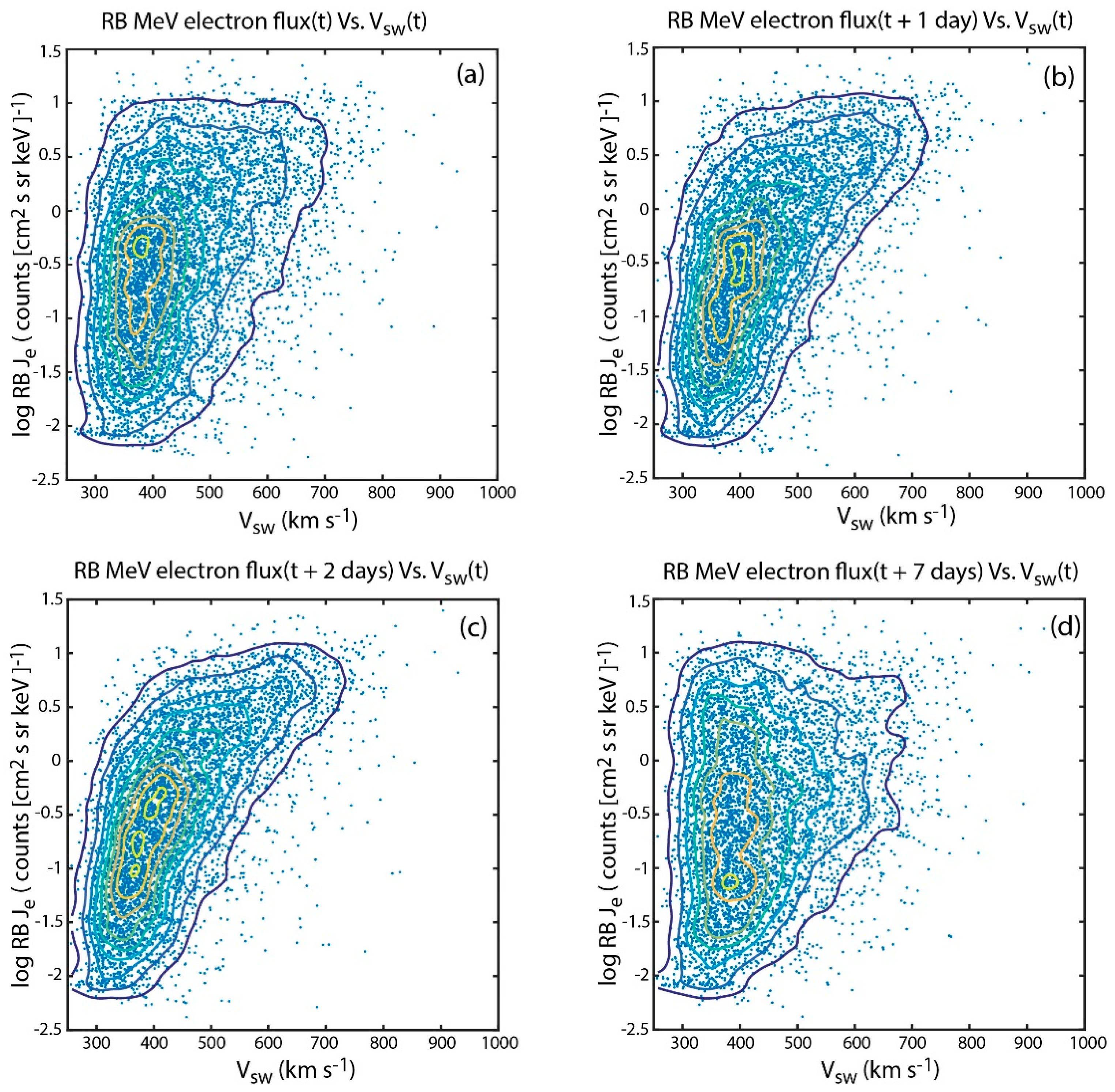
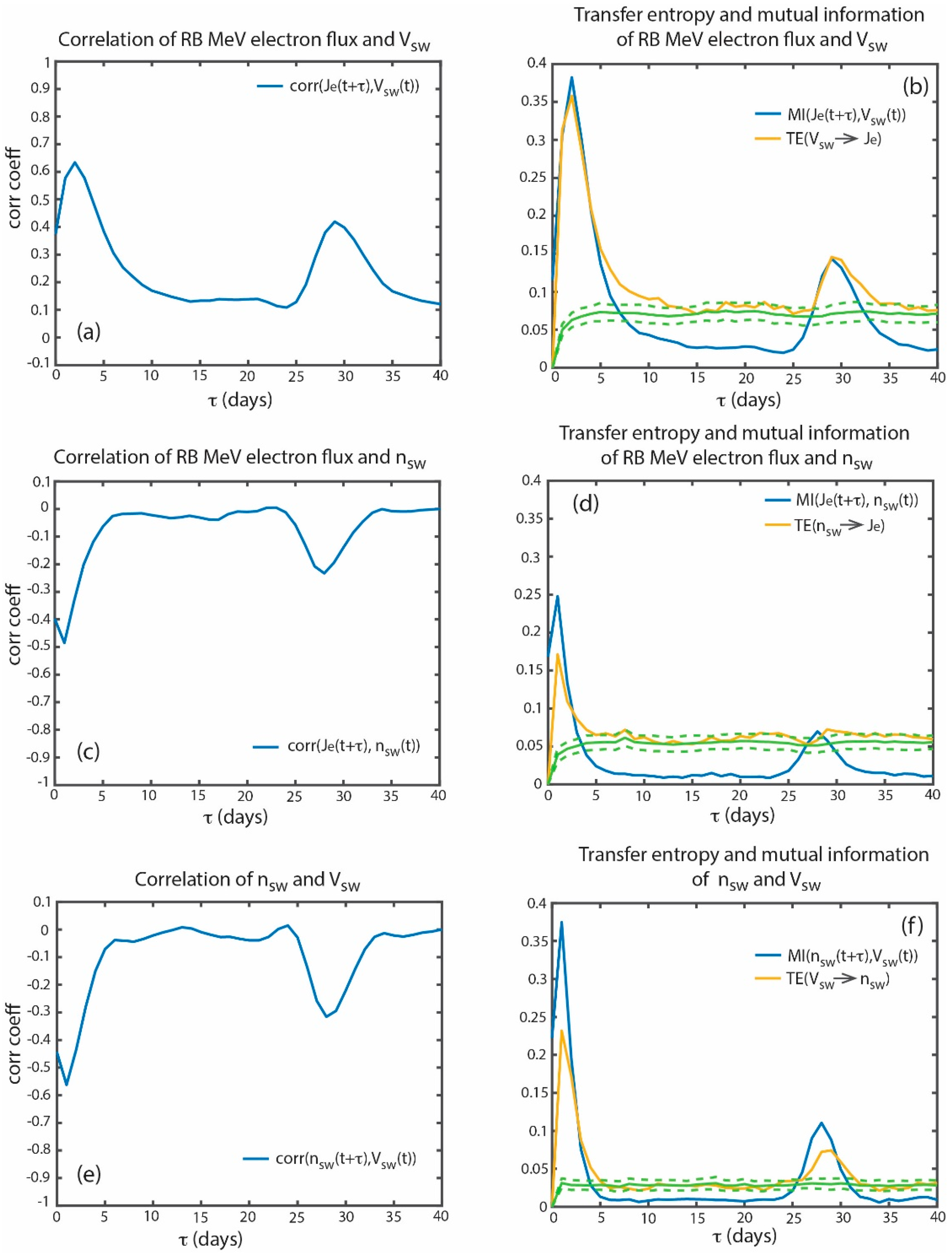
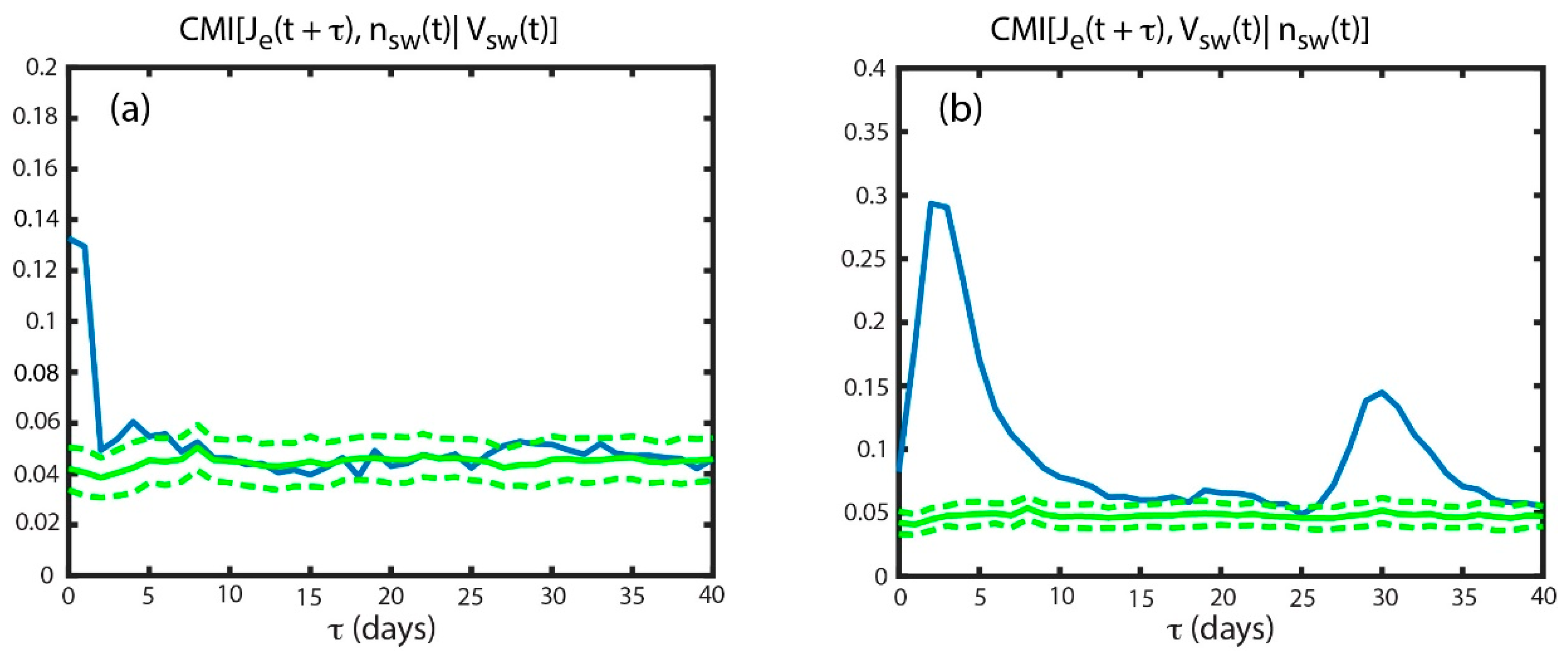
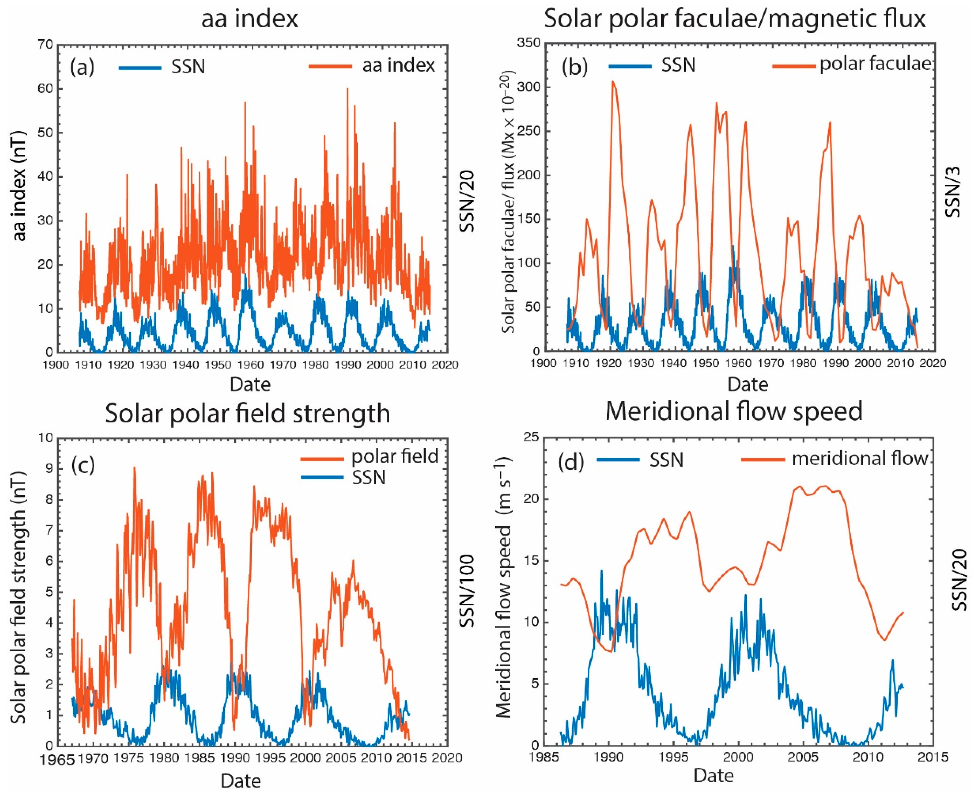
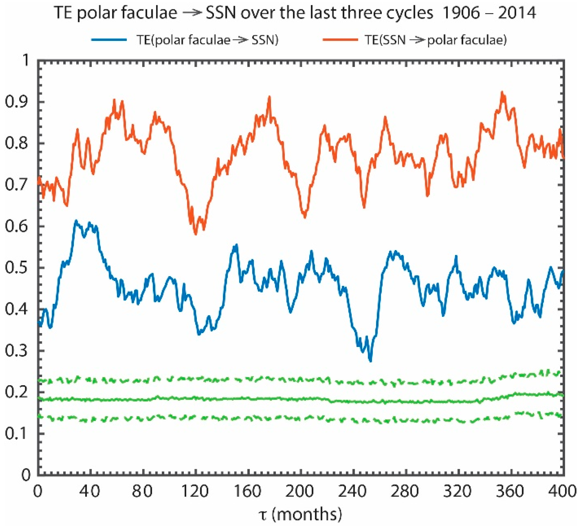
Table 1.
Ranking of the solar wind parameters based on information transfer to geosynchronous Mev electron flux (Je) at τmax, where τmax is the lag time when the information transfer peaks. Parameters 2–9 are calculated from CMI[Je(t + τ), x(t) | Vsw(t)] whereas parameter 1 is calculated from CMI[Je(t + τ), Vsw(t) | nsw(t)], where x = parameter 2–9. The peak information transfer (itmax) = peak – mean noise, the signal to noise ratio = peak/noise, and significance = itmax/σ(noise). Noise is calculated from surrogate data (see Section 4). The prediction horizon gives the lag time when there is no information transfer from the solar wind parameter to Je. Note that nsw and Pdyn are both ranked at number 3 because they have similar itmax (the effect of Vsw has been removed). * excluding the effect of solar rotation. (from [23].)
| Rank | Solar Wind Parameters | Peak Information Transfer (itmax) | Signal to Noise Ratio at τmax | Significance at τmax (σ) | τmax (Days) | Prediction Horizon (Days) |
|---|---|---|---|---|---|---|
| 1 | Vsw | 0.25 | 6.6 | 94 | 2 | 10 * |
| 2 | IMF |B| | 0.12 | 3.9 | 48 | 0 | 2 |
| 3 | Pdyn | 0.092 | 3.4 | 35 | 0 | 2 |
| 3 | nsw | 0.091 | 3.2 | 34 | 0 | 2 |
| 4 | σ(IMF B) | 0.075 | 3.9 | 48 | 0 | 2 |
| 5 | IMF Bz < 0 | 0.064 | 2.7 | 26 | 0 | 2 |
| 6 | Esw | 0.056 | 2.9 | 22 | 1 | 5 |
| 7 | IMF By | 0.052 | 2.3 | 20 | 0 | 2 |
| 8 | IMF Bz > 0 | 0.048 | 3.1 | 22 | 0 | 2 |
| 9 | IMF Bx | 0.044 | 2.2 | 19 | 0 | 2 |
© 2019 by the authors. Licensee MDPI, Basel, Switzerland. This article is an open access article distributed under the terms and conditions of the Creative Commons Attribution (CC BY) license (http://creativecommons.org/licenses/by/4.0/).
Share and Cite
MDPI and ACS Style
Wing, S.; Johnson, J.R. Applications of Information Theory in Solar and Space Physics. Entropy 2019, 21, 140. https://doi.org/10.3390/e21020140
AMA Style
Wing S, Johnson JR. Applications of Information Theory in Solar and Space Physics. Entropy. 2019; 21(2):140. https://doi.org/10.3390/e21020140
Chicago/Turabian StyleWing, Simon, and Jay R. Johnson. 2019. "Applications of Information Theory in Solar and Space Physics" Entropy 21, no. 2: 140. https://doi.org/10.3390/e21020140
Note that from the first issue of 2016, this journal uses article numbers instead of page numbers. See further details here.