Magnetic Otto Engine for an Electron in a Quantum Dot: Classical and Quantum Approach

 ,
,  , ,
, , 
Abstract
:1. Introduction
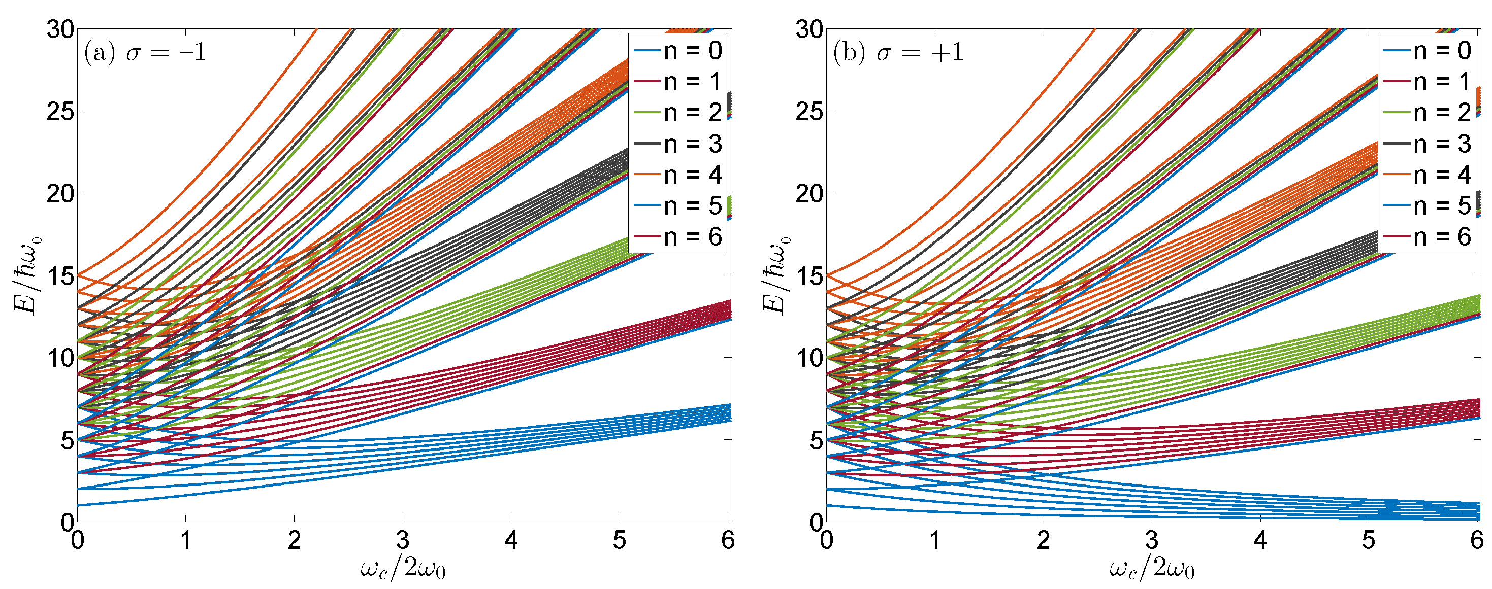
2. Model
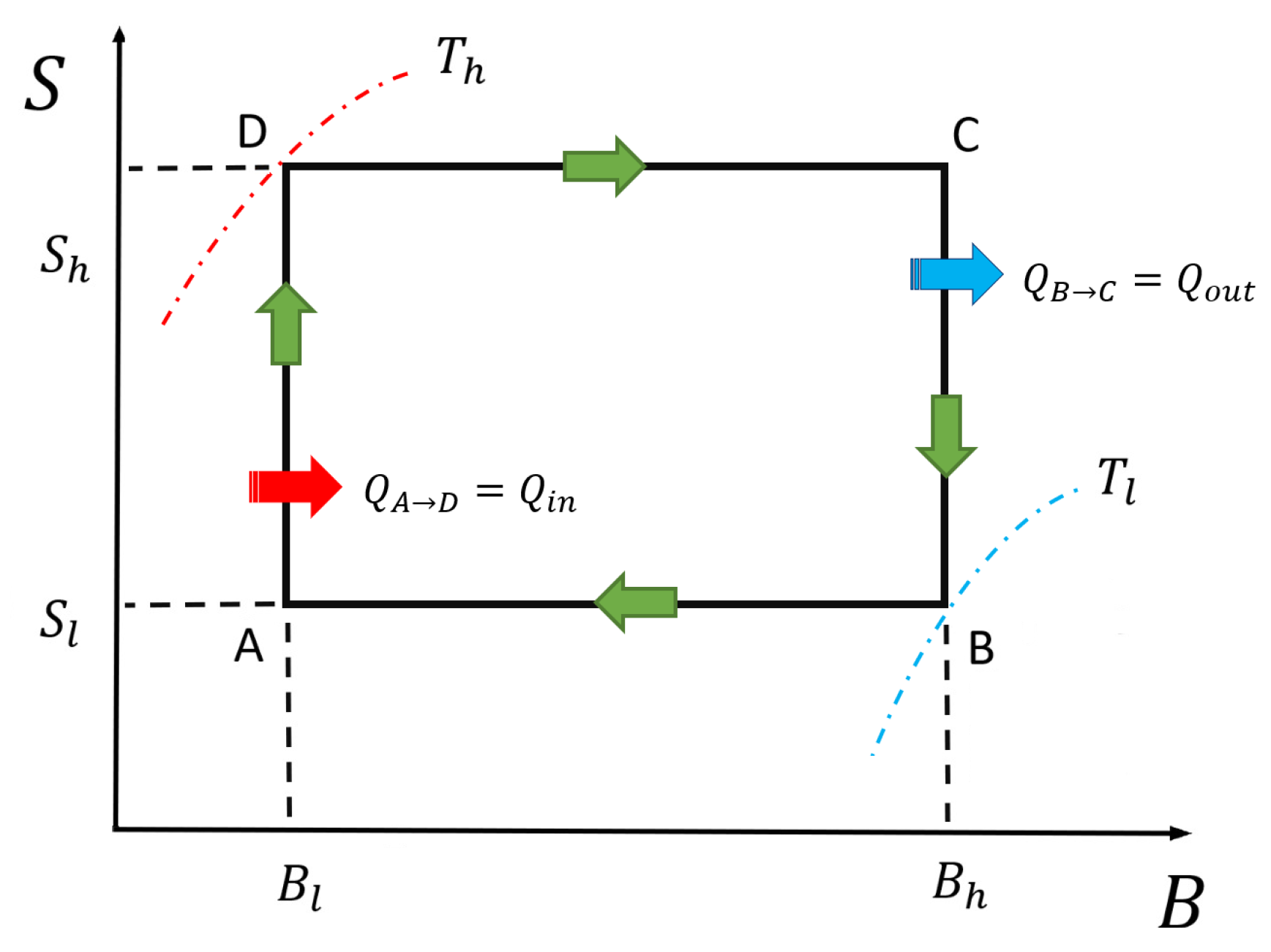
3. First Law of Thermodynamics and the Quantum and Classical Otto Cycle
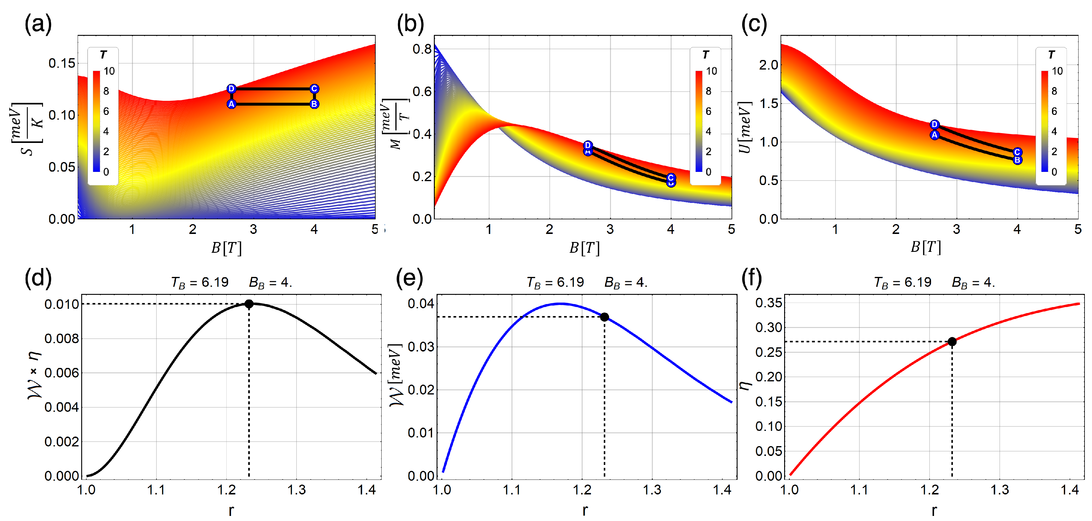
- Finding the relation between the magnetic field and the temperature along an isentropic trajectory by solving the differential equation of first order given bywhich can be written aswhere is the specific heat at constant magnetic field.
- By matching two points within an isentropic trajectoryfinding the magnetic field in terms of the temperature, throughout numerical calculation.
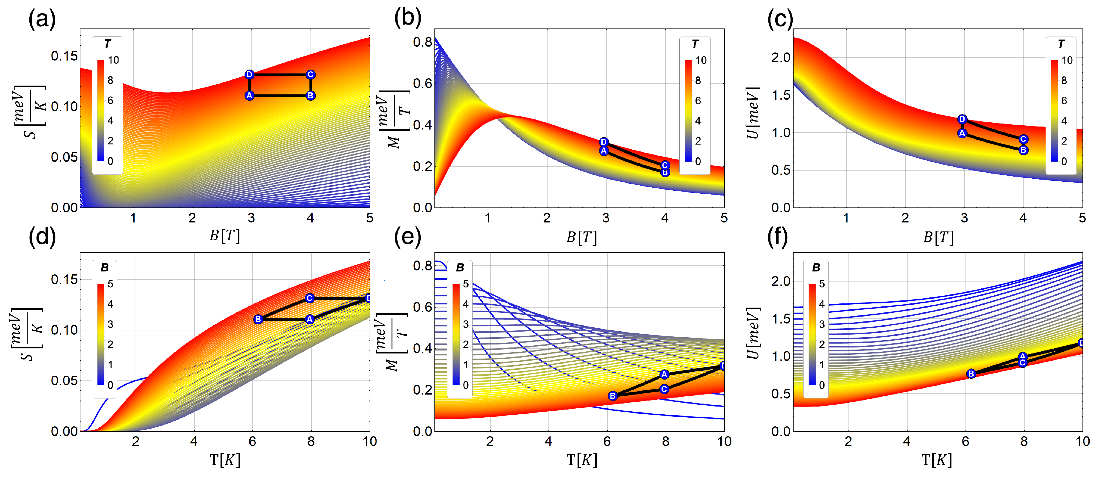
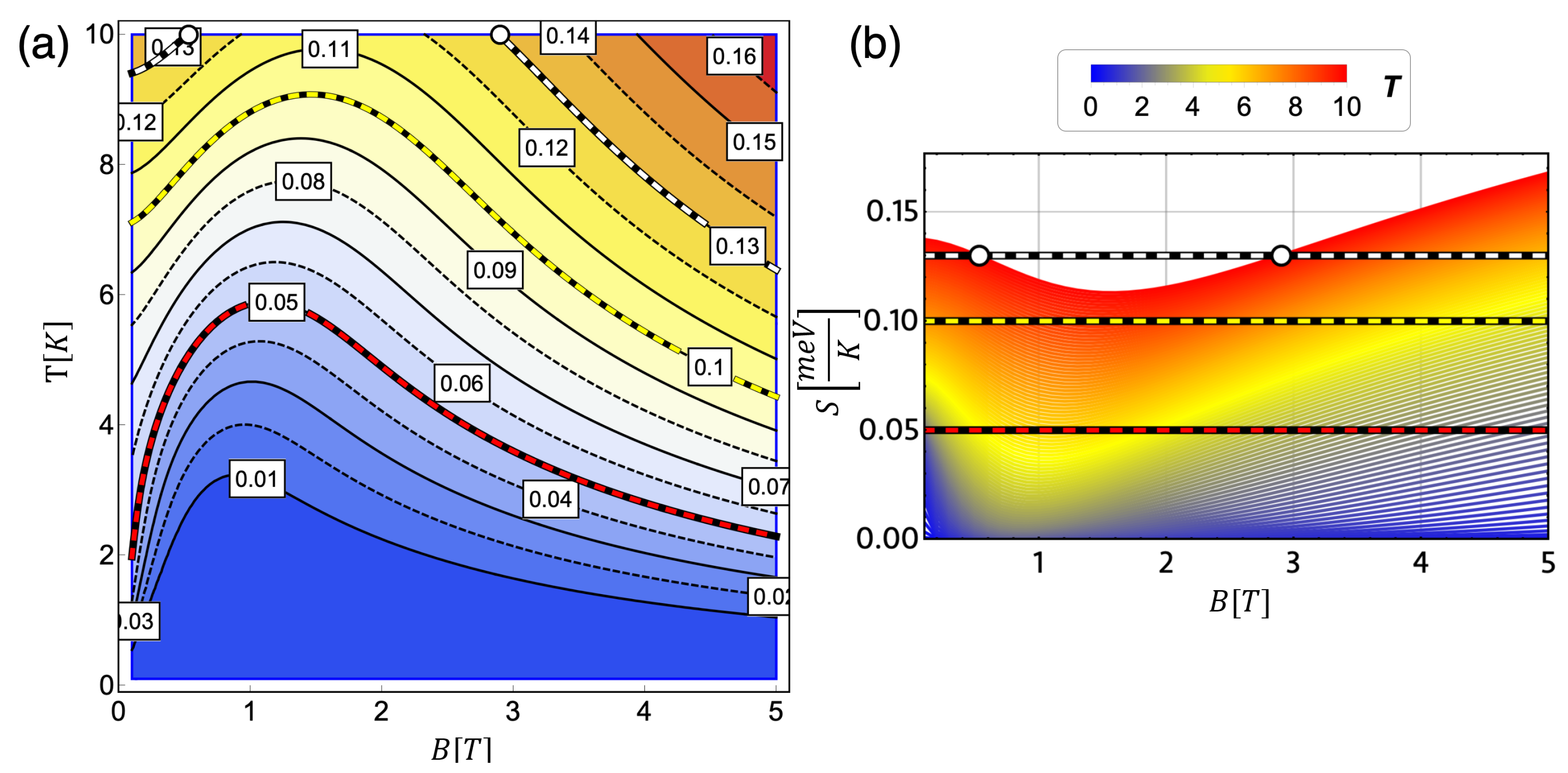
4. Results and Discussions
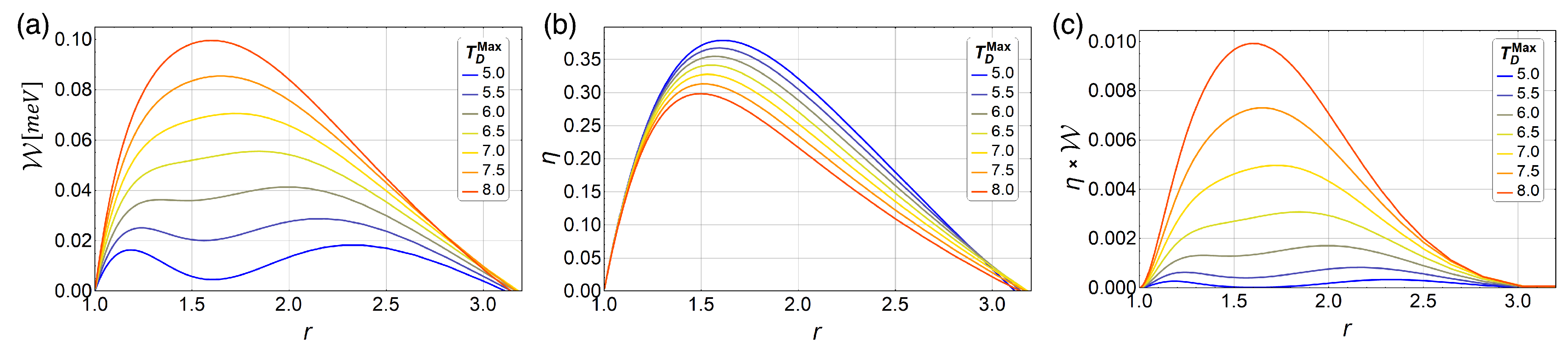
4.1. Classical Magnetic Otto Cycle
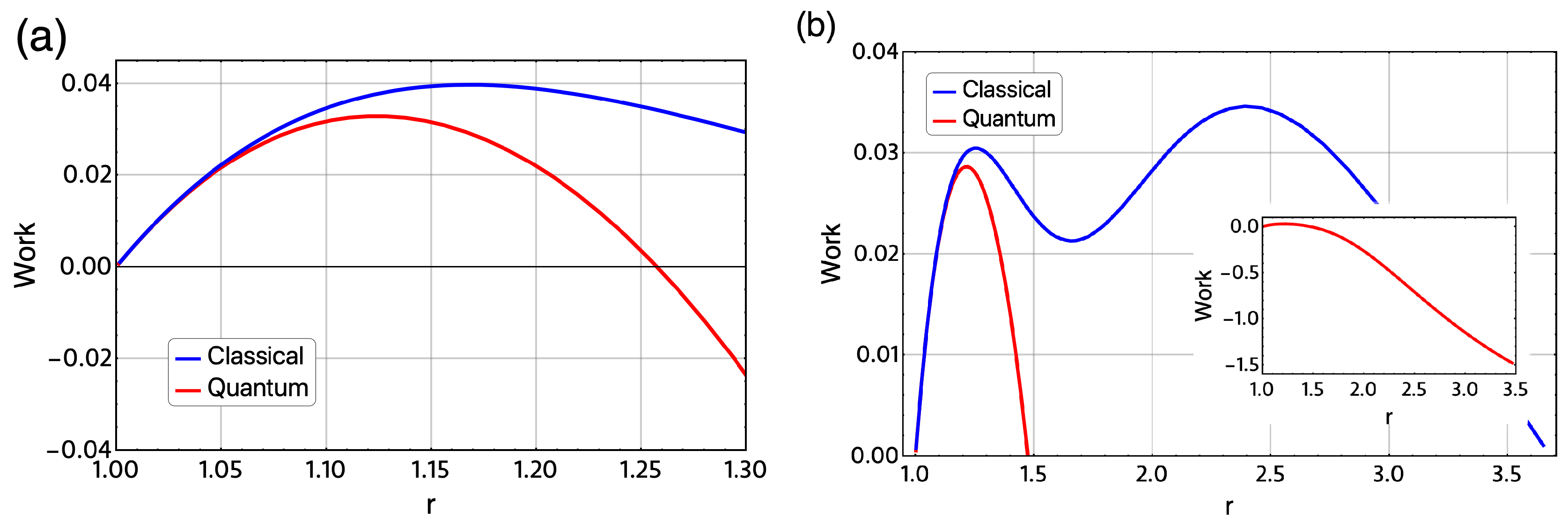
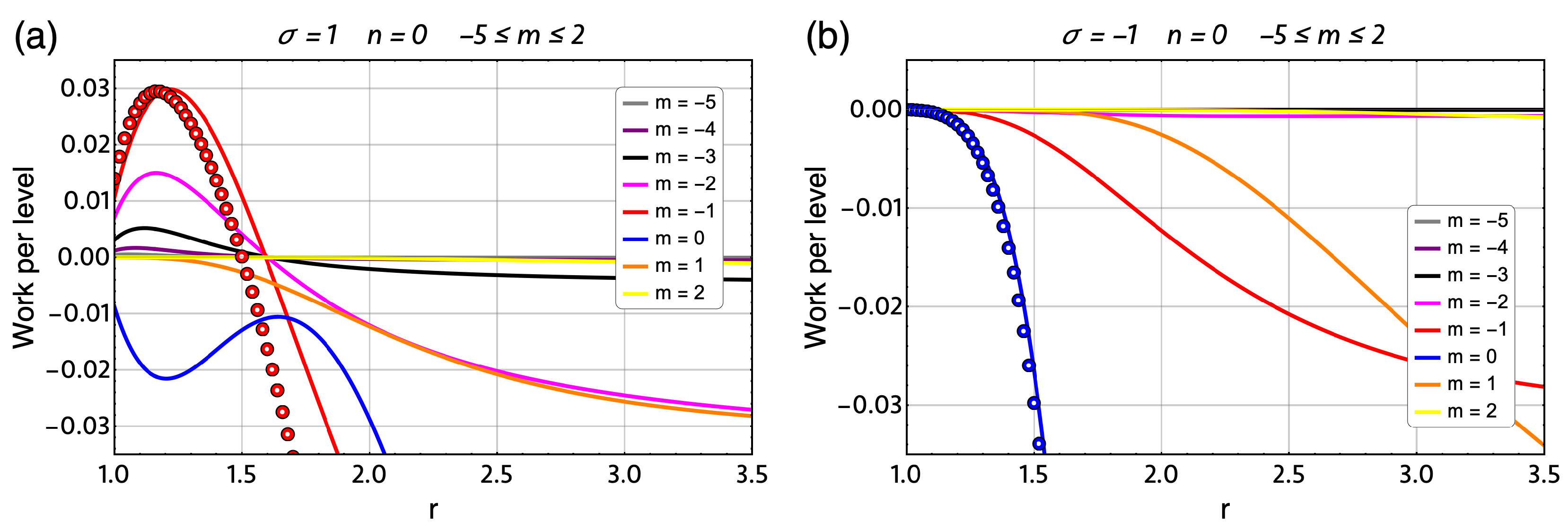
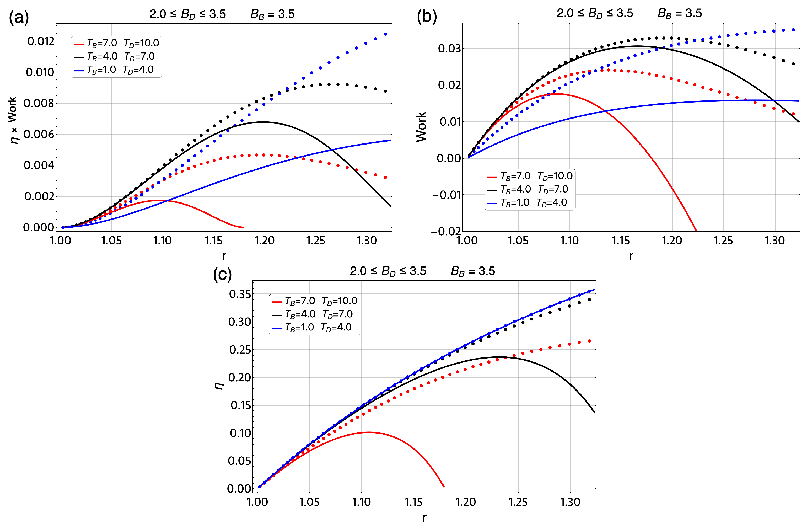
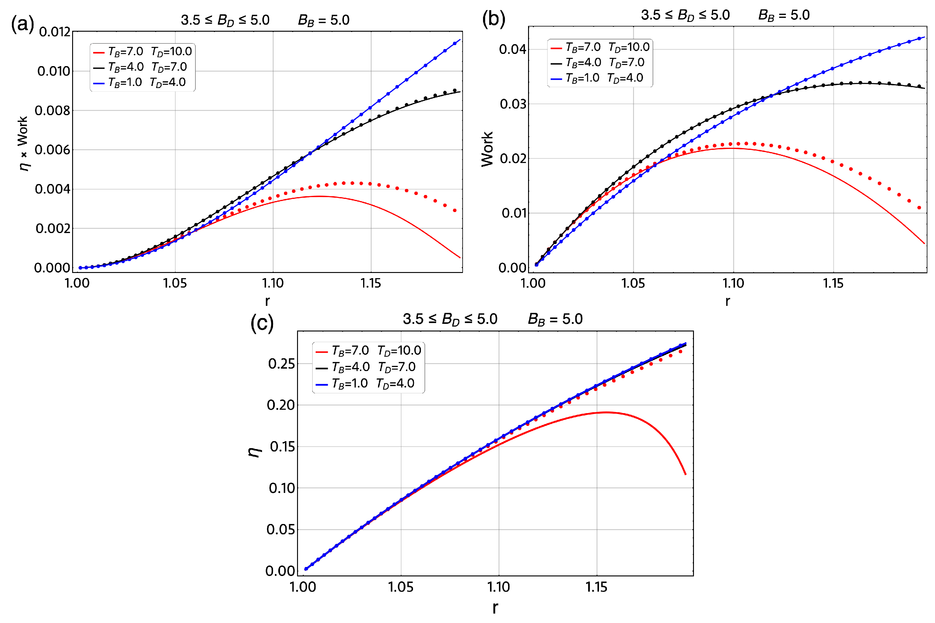
4.2. Magnetic Quantum Otto Cycle
5. Conclusions
Supplementary Materials
Author Contributions
Funding
Acknowledgments
Conflicts of Interest
References
- Scovil, H.E.D.; Schulz-DuBois, D.O. Three-Level masers as a heat engines. Phys. Rev. Lett. 1959, 2, 262–263. [Google Scholar] [CrossRef]
- Feldmann, T.; Geva, E.; Kosloff, R.; Salamon, P. Heat engines in finite time governed by master equations. Am. J. Phys. 1996, 64, 485. [Google Scholar] [CrossRef]
- Feldmann, T.; Kosloff, R. Characteristics of the limit cycle of a reciprocating quantum heat engine. Phys. Rev. E 2004, 70, 046110. [Google Scholar] [CrossRef]
- Rezek, Y.; Kosloff, R. Irreversible performance of a quantum harmonic heat engine. New J. Phys. 2006, 8, 83. [Google Scholar] [CrossRef]
- Henrich, M.J.; Rempp, F.; Mahler, G. Quantum thermodynamic Otto machines: A spin-system approach. Eur. Phys. J. Spec. Top. 2007, 151, 157. [Google Scholar] [CrossRef]
- Quan, H.T.; Liu, Y.-X.; Sun, C.P.; Nori, F. Quantum thermodynamic cycles and quantum heat engines. Phys. Rev. E 2007, 76, 031105. [Google Scholar] [CrossRef]
- He, J.; He, X.; Tang, W. The performance characteristics of an irreversible quantum Otto harmonic refrigeration cycle. Sci. China Ser. G Phy. Mech. Astron. 2009, 52, 1317. [Google Scholar] [CrossRef]
- Liu, S.; Ou, C. Maximum Power Output of Quantum Heat Engine with Energy Bath. Entropy 2016, 18, 205. [Google Scholar] [CrossRef]
- Scully, M.O.; Zubairy, M.S.; Agarwal, G.S.; Walther, H. Extracting work from a single heath bath via vanishing quantum coherence. Science 2003, 299, 862–864. [Google Scholar] [CrossRef]
- Scully, M.O.; Zubairy, M.S.; Dorfmann, K.E.; Kim, M.B.; Svidzinsky, A. Quantum heat engine power can be increased by noise-induced coherence. Proc. Natl. Acad. Sci. USA 2011, 108, 15097–15100. [Google Scholar] [CrossRef]
- Bender, C.M.; Brody, D.C.; Meister, B.K. Quantum mechanical Carnot engine. J. Phys. A Math. Gen. 2000, 33, 4427. [Google Scholar] [CrossRef]
- Bender, C.M.; Brody, D.C.; Meister, B.K. Entropy and temperature of quantum Carnot engine. Proc. R. Soc. Lond. A 2002, 458, 1519. [Google Scholar] [CrossRef]
- Wang, J.H.; Wu, Z.Q.; He, J. Quantum Otto engine of a two-level atom with single-mode fields. Phys. Rev. E 2012, 85, 041148. [Google Scholar] [CrossRef]
- Huang, X.L.; Xu, H.; Niu, X.Y.; Fu, Y.D. A special entangled quantum heat engine based on the two-qubit Heisenberg XX model. Phys. Scr. 2013, 88, 065008. [Google Scholar] [CrossRef]
- Muñoz, E.; Peña, F.J. Quantum heat engine in the relativistic limit: The case of Dirac particle. Phys. Rev. E 2012, 86, 061108. [Google Scholar] [CrossRef] [PubMed]
- Quan, H.T. Quantum thermodynamic cycles and quantum heat engines (II). Phys. Rev. E 2009, 79, 041129. [Google Scholar] [CrossRef]
- Zheng, Y.; Polleti, D. Work and efficiency of quantum Otto cycles in power-law trapping potentials. Phys. Rev. E 2014, 90, 012145. [Google Scholar] [CrossRef]
- Cui, Y.Y.; Chem, X.; Muga, J.G. Transient Particle Energies in Shortcuts to Adiabatic Expansions of Harmonic Traps. J. Phys. Chem. A 2016, 120, 2962. [Google Scholar] [CrossRef] [PubMed]
- Beau, M.; Jaramillo, J.; del Campo, A. Scaling-up Quantum Heat Engines Efficiently via Shortcuts to Adiabaticity. Entropy 2016, 18, 168. [Google Scholar] [CrossRef]
- Deng, J.; Wang, Q.; Liu, Z.; Hänggi, P.; Gong, J. Boosting work characteristics and overall heat-engine performance via shortcuts to adibaticity: Quantum and classical systems. Phys. Rev. E 2013, 88, 062122. [Google Scholar] [CrossRef] [PubMed]
- Wang, J.; He, J.; He, X. Performance analysis of a two-state quantum heat engine working with a single-mode radiation field in a cavity. Phys. Rev. E 2011, 84, 041127. [Google Scholar] [CrossRef]
- Abe, S. Maximum-power quantum-mechanical Carnot engine. Phys. Rev. E 2011, 83, 041117. [Google Scholar] [CrossRef]
- Wang, J.H.; He, J.Z. Optimization on a three-level heat engine working with two noninteracting fermions in a one-dimensional box trap. J. Appl. Phys. 2012, 111, 043505. [Google Scholar] [CrossRef]
- Wang, R.; Wang, J.; He, J.; Ma, Y. Performance of a multilevel quantum heat engine of an ideal N-particle Fermi system. Phys. Rev. E 2012, 86, 021133. [Google Scholar] [CrossRef]
- Jaramillo, J.; Beau, M.; del Campo, A. Quantum supremacy of many-particle thermal machines. New J. Phys. 2016, 18, 075019. [Google Scholar] [CrossRef]
- Del Campo, A.; Goold, J.; Paternostro, M. More bang for your buck: Super-adiabatic quantum engines. Sci. Rep. 2017, 4, 14391. [Google Scholar] [CrossRef]
- Huang, X.L.; Niu, X.Y.; Xiu, X.M.; Yi, X.X. Quantum Stirling heat engine and refrigerator with single and coupled spin systems. Eur. Phys. J. D 2014, 68, 32. [Google Scholar] [CrossRef]
- Su, S.H.; Luo, X.Q.; Chen, J.C.; Sun, C.P. Angle-dependent quantum Otto heat engine based on coherent dipole-dipole coupling. EPL 2016, 115, 30002. [Google Scholar] [CrossRef]
- Kosloff, R.; Rezek, Y. The Quantum Harmonic Otto Cycle. Entropy 2017, 19, 136. [Google Scholar] [CrossRef]
- Klatzow, J.; Becker, J.N.; Ledingham, P.M.; Weinzetl, C.; Kaczmarek, K.T.; Saunders, D.J.; Nunn, J.; Walmsley, I.A.; Uzdin, R.M.; Poem, E. Experimental demonstration of quantum effects in the operation of microscopic heat engines. arXiv 2017, arXiv:1710.08716v2. [Google Scholar] [CrossRef]
- Peterson, J.P.S.; Batalhão, T.B.; Herrera, M.; Souza, A.M.; Sarthour, R.S.; Oliveira, I.S.; Serra, R.M. Experimental characterization of a spin quantum heat engine. arXiv 2018, arXiv:1803.06021v1. [Google Scholar]
- Von Lindenfels, D.; Gräb, O.; Schmiegelow, C.T.; Kaushal, V.; Schulz, J.; Schmidt-Kaler, F.; Poschinger, U.G. A spin heat engine coupled to a harmonic-oscillator flywheel. arXiv 2018, arXiv:1808.02390v1. [Google Scholar]
- Van Horne, N.; Yum, D.; Dutta, T.; Hänggi, P.; Gong, J.; Poletti, D.; Mukherjee, M. Single atom energy-conversion device with a quantum load. arXiv 2018, arXiv:1808.02390v1. [Google Scholar]
- Roßnagel, J.; Dawkins, T.K.; Tolazzi, N.K.; Abah, O.; Lutz, E.; Kaler-Schmidt, F.; Singer, K.A. Single-atom heat engine. Science 2016, 352, 325. [Google Scholar] [CrossRef]
- Dong, C.D.; Lefkidis, G.; Hübner, W. Quantum Isobaric Process in Ni2. J. Supercond. Nov. Magn. 2013, 26, 1589–1594. [Google Scholar] [CrossRef]
- Dong, C.D.; Lefkidis, G.; Hübner, W. Magnetic quantum diesel in Ni2. Phys. Rev. B 2013, 88, 214421. [Google Scholar] [CrossRef]
- Hübner, W.; Lefkidis, G.; Dong, C.D.; Chaudhuri, D. Spin-dependent Otto quantum heat engine based on a molecular substance. Phys. Rev. B 2014, 90, 024401. [Google Scholar] [CrossRef]
- Mehta, V.; Johal, R.S. Quantum Otto engine with exchange coupling in the presence of level degeneracy. Phys. Rev. E 2017, 96, 032110. [Google Scholar] [CrossRef]
- Azimi, M.; Chorotorlisvili, L.; Mishra, S.K.; Vekua, T.; Hübner, W.; Berakdar, J. Quantum Otto heat engine based on a multiferroic chain working substance. New J. Phys. 2014, 16, 063018. [Google Scholar] [CrossRef]
- Chotorlishvili, L.; Azimi, M.; Stagraczyński, S.; Toklikishvili, Z.; Schüler, M.; Berakdar, J. Superadiabatic quantum heat engine with a multiferroic working medium. Phys. Rev. E 2016, 94, 032116. [Google Scholar] [CrossRef]
- Muñoz, E.; Peña, F.J. Magnetically driven quantum heat engine. Phys. Rev. E 2014, 89, 052107. [Google Scholar] [CrossRef]
- Alecce, A.; Galve, F.; Gullo, N.L.; Dell’Anna, L.; Plastina, F.; Zambrini, R. Quantum Otto cycle with inner friction: Finite-time and disorder effects. New J. Phys. 2015, 17, 075007. [Google Scholar] [CrossRef]
- Brandner, K.; Bauer, M.; Seifert, U. Universal Coherence-Induced Power Losses of Quantum Heat Engines in Linear Response. Phys. Rev. Lett. 2017, 119, 170602. [Google Scholar] [CrossRef]
- Feldmann, T.; Koslof, R. Performance of discrete heat engines and heat pumps in finite time. Phys. Rev. E 2000, 61, 4774. [Google Scholar] [CrossRef]
- Feldmann, T.; Koslof, R. Transitions between refrigeration regions in extremely short quantum cycles. Phys. Rev. E 2016, 93, 052150. [Google Scholar] [CrossRef] [PubMed]
- Pekola, J.P.; Karimi, B.; Thomas, G.; Averin, D.V. Supremacy of incoherent sudden cycles cycles. arXiv 2018, arXiv:1812.10933v1. [Google Scholar]
- Jacak, L.; Hawrylak, P.; Wójs, A. Quantum Dots; Springer: New York, NY, USA, 1998. [Google Scholar]
- Muñoz, E.; Barticevic, Z.; Pacheco, M. Electronic spectrum of a two-dimensional quantum dot array in the presence of electric and magnetic fields in the Hall configuration. Phys. Rev. B 2005, 71, 165301. [Google Scholar] [CrossRef]
- Mani, R.G.; Smet, J.H.; von Klitzing, K.; Narayanamurti, V.; Johnson, W.B.; Umansky, V. Zero-resistance states induced by electromagnetic-wave excitation in GaAs/AlGaAs heterostructures. Nature 2002, 420, 646–650. [Google Scholar] [CrossRef]
- Quan, H.T.; Zhang, P.; Sun, C.P. Quantum heat engine with multilevel quantum systems. Phys. Rev. E 2005, 72, 056110. [Google Scholar] [CrossRef]
- Peña, F.J.; Muñoz, E. Magnetostrain-driven quantum heat engine on a graphene flake. Phys. Rev. E 2015, 91, 052152. [Google Scholar] [CrossRef]
- Muñoz, E.; Peña, F.J.; González, A. Magnetically-Driven Quantum Heat Engines: The Quasi-Static Limit of Their Efficiency. Entropy 2016, 18, 173. [Google Scholar] [CrossRef]
- Callen, H.B. Thermodynamics and an Introduction to Thermostatistics; John Wiley & Sons: New York, NY, USA, 1985. [Google Scholar]
- Kumar, J.; Sreeram, P.A.; Dattagupta, S. Low-temperature thermodynamics in the context of dissipative diamagnetism. Phys. Rev. E 2009, 79, 021130. [Google Scholar] [CrossRef]
- Wolfram Research, Inc. Mathematica; Version 11.3; Wolfram Research, Inc.: Champaign, IL, USA, 2018. [Google Scholar]


© 2019 by the authors. Licensee MDPI, Basel, Switzerland. This article is an open access article distributed under the terms and conditions of the Creative Commons Attribution (CC BY) license (http://creativecommons.org/licenses/by/4.0/).
Share and Cite
Peña, F.J.; Negrete, O.; Alvarado Barrios, G.; Zambrano, D.; González, A.; Nunez, A.S.; Orellana, P.A.; Vargas, P. Magnetic Otto Engine for an Electron in a Quantum Dot: Classical and Quantum Approach. Entropy 2019, 21, 512. https://doi.org/10.3390/e21050512
Peña FJ, Negrete O, Alvarado Barrios G, Zambrano D, González A, Nunez AS, Orellana PA, Vargas P. Magnetic Otto Engine for an Electron in a Quantum Dot: Classical and Quantum Approach. Entropy. 2019; 21(5):512. https://doi.org/10.3390/e21050512
Chicago/Turabian StylePeña, Francisco J., Oscar Negrete, Gabriel Alvarado Barrios, David Zambrano, Alejandro González, Alvaro S. Nunez, Pedro A. Orellana, and Patricio Vargas. 2019. "Magnetic Otto Engine for an Electron in a Quantum Dot: Classical and Quantum Approach" Entropy 21, no. 5: 512. https://doi.org/10.3390/e21050512
APA StylePeña, F. J., Negrete, O., Alvarado Barrios, G., Zambrano, D., González, A., Nunez, A. S., Orellana, P. A., & Vargas, P. (2019). Magnetic Otto Engine for an Electron in a Quantum Dot: Classical and Quantum Approach. Entropy, 21(5), 512. https://doi.org/10.3390/e21050512