Ordinal Patterns in Heartbeat Time Series: An Approach Using Multiscale Analysis

Departamento de Matemática Aplicada y Estadística, Universidad Politécnica de Cartagena, 30202 Cartagena, Spain
Entropy 2019, 21(6), 583; https://doi.org/10.3390/e21060583
Submission received: 17 May 2019
/
Revised: 6 June 2019
/
Accepted: 7 June 2019
/
Published: 12 June 2019
(This article belongs to the Special Issue Theoretical Developments and Applications of Entropy and Ordinal Patterns)
Abstract
:In this paper, we simultaneously use two different scales in the analysis of ordinal patterns to measure the complexity of the dynamics of heartbeat time series. Rényi entropy and weighted Rényi entropy are the entropy-like measures proposed in the multiscale analysis in which, with the new scheme, four parameters are involved. First, the influence of the variation of the new parameters in the entropy values is analyzed when different groups of subjects (with cardiac diseases or healthy) are considered. Secondly, we exploit the introduction of multiscale analysis in order to detect differences between the groups.
1. Introduction
Entropy-like measures are a powerful tool in the study of time series. The encoded information in a time series has turned out to be a valuable source of information. Since the seminal paper of Bandt and Pompe in 2002 [1], permutation entropy (PE) has been used to measure the complexity of different types of processes, since the order relation established in the time series allows finding patterns linking with the complexity of the system; see [2] for a review about permutation entropy and its applications. In particular, biomedical time series have been the focus of great interest, including neuronal signals and heart rate series [3]. Nevertheless, new variants of entropy-like measures have arisen in the last years, considering the nature of the series that is object of study [4], since differences appear when we consider different versions of entropy and different values of the parameters. Therefore, the analysis of the behavior of each of them, taking into account the final purpose that has been fixed, is relevant.
A natural approach to the study of possible cardiac problems is the analysis of heartbeat series. The activity of human beings influences heartbeat series, causing non-stationary series in healthy subjects. Cardiac diseases should be revealed in heartbeat series though significant changes in complexity. Difficulties in measuring that complexity have been considered and preliminary results can be found in different papers where the idea of extracting information from the time series is presented. Thus, Pincus and collaborators use approximate entropy (AE) in several papers to quantify the complexity and the regularity of biological time series [5,6]. In [7], symbolic dynamics and renormalized entropy were used to detect abnormalities in heart rate variability (HRV) in patients that had been classified as low-risk using traditional methods. In 2002, [8] a sample entropy analysis of neonatal heart rate variability was considered, taking into account the abnormal heart rate characteristics appearing in neonatal sepsis. Atrial fibrillation (AF) is a common cardiac arrhythmia in which irregular patterns of electrical activation are usually found in the atria [9]. Cammarota and Rogora (2005) studied the independence of non-stationary heartbeat series during atrial fibrillation (AF) comparing two methods, one using a linear Gaussian state space model and the other using symbolic permutation [10].
In [11], a complexity analysis of heart period variability under two different approaches was considered. The typification of complexity in short heart period variability series was done using Shannon entropy (SE) and conditional entropy (CE), the work concluded that the study of complexity can be very useful in the diagnosis of arrhythmias.
Entropy measures, approximate entropy (AE), sample entropy (SamE), fuzzy entropy (FE), and permutation entropy (PE) were computed for short EGG series in [12] in order to separate healthy patients and patients with congestive heart failure. In [13], Zunino and collaborators used permutation min-entropy (PME) in order to discriminate patients with AF. Recently, in 2018, permutation entropy and min-entropy in a heartbeat time series were applied to detect changes in the emotional states of subjects [14].
The quantification of the regularity in time series is the basic idea that underlies in this framework. The advantages of permutation entropy as a good measure of regular behavior and the simple, fast, and easy implementation and robustness and invariance with respect to non-linear monotonous transformations, see [1], makes it a valuable tool to analyze time series. Nevertheless, it is not clear what the best entropy-like measure to incorporate it is. The number of different entropy-like measures and the nature of the heartbeat series means that the election of an entropy-like measure good enough for measuring the complexity of the dynamics is non-trivial. Thus, Costa [15] highlighted that multiple time scales are inherent in healthy physiologic dynamics, and multiscale entropy can be adapted to study these types of processes. In particular, in [15] multiscale sample entropy is applied. On the other hand, other parameters should be taken into account to establish critical points in different groups of subjects for a more accurate discrimination. In fact, the delay parameter is in many situations fixed as and is not included in the analysis, but this parameter can be non-trivial when we are considering heartbeat interval series, as has been highlighted in [13].
Our approach is aimed at analyzing different types of heartbeat series of 24 h for patients of three different groups (a congestive heart failure (CHF) group, healthy (H) group, and atrial fibrillation (AF) group) using multiscale analysis and discarding additional information with additional delay using Rényi permutation entropy (RPE), since this entropy-like measure has reported the best results in some biological processes [16], as well as weighted Rényi entropy. This means that two parameters are added to the original entropy-like measure that needs two parameters, namely, the embedding dimension m and the parameter associated with the Rényi parameter , (recall that privileges rare events while does the same for frequent events). When the parameter tends to 1, we obtain PE entropy. Summing up, four parameters are involved in multiscale Rényi permutation entropy (MRPE): the scale s, the delay , the embedding dimension m, and the Rényi parameter . Analogously, weighted permutation entropy provides more control between the differences in the patterns, thus we include weighted multiscale Rényi entropy (WMRPE) parallel to (MRPE), as has been suggested in [17], where this scheme has been applied to the analysis of economic series; in particular, the analysis was focused on the closing prices of financial stock markets of different areas. Thus, we will simultaneously use two different scales in our analysis.
We consider the data freely available at http://www.physione.org/challenge/chaos, where a challenge entitled “Is the Normal Heart Rate Chaotic?” was launched and heart beat time series from 15 subjects are provided. Five of them correspond to patients suffering congestive heart failure (CHF), five come from subjects suffering atrial fibrillation (AF), and finally a group of five healthy subjects allows us to compare the results (control group). Our efforts are aimed at assessing if it is worth introducing multiscale analysis in heart time series. Hence, we will determine if any change and differences are detected when a multiscale analysis is added.
2. Terminology and Notation: Ordinal Patterns
Although most of the notions are well known, we recall them for the sake of completeness. The definitions that follow, with slightly differences, can be found in the literature; see for instance [1,3,4,18,19]. The starting point is a real time series where ordinal patterns of length m are considered. The length of the series must be big enough, since the procedure of reconstruction of the attractor evaluating the associated probability distribution requires enough data. Following [20], a required condition is .
Let be a fixed natural number, be the group of permutations of length m, and . The vector is said to be -type if
and
if for . Observe that the number of possible ordinal patterns of length m is given by the cardinality of , that is .
The length of the patterns is called the embedding dimension. Following [1], low orders of m are recommended for practical purposes. We will use , and 5.
The following definition, where delay parameter is included, gives the relative frequency of the pattern associated with the permutation .
Definition 1
Permutation entropy (PE) was defined by Bandt and Pompe [1]. Let be a real time series, . Then the permutation entropy (PE) is given by
where and . The Rényi entropy variant [21] generalizes the permutation entropy [22]. The definition follows; see for instance [4] (Definition 4).
Definition 2.
Let be a time series, , . Then, the Rényi permutation entropy of (RPE), is given by
where is given as in Definition 1. When the parameters are fixed, we write RPE for short.
Permutation entropy (PE), also called Shannon entropy (SE), is obtained when tends to 1 in Rényi permutation entropy. Liang [16] reported that the class of permutation entropy with the best results when EEG during different anesthesia states are considered is Rényi entropy. Moreover, the choice of the parameter is not a trivial question; see [23].
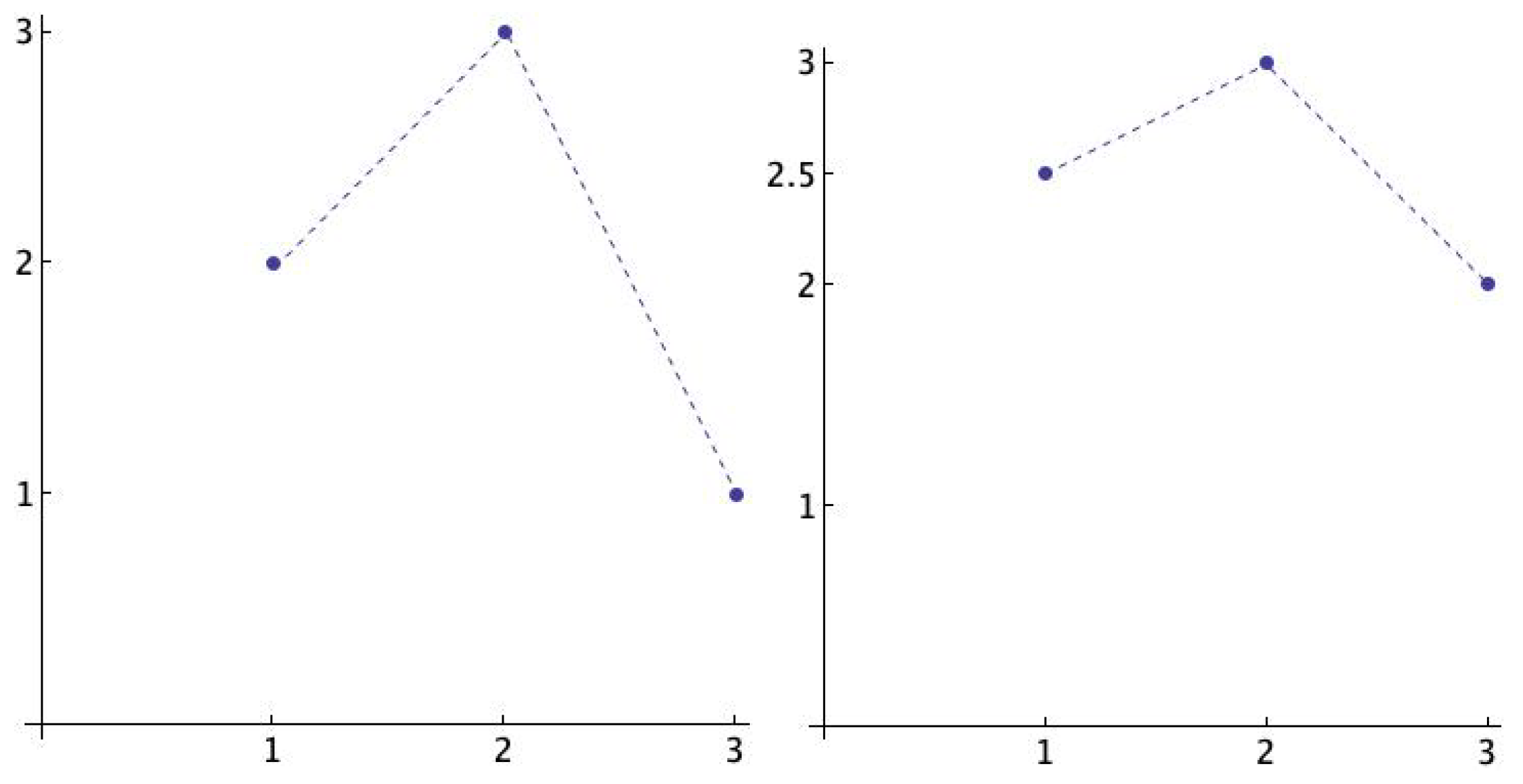
The weighted version of Rényi entropy uses weighted frequencies in which not only the order is considered but also the differences between the values of the pattern. The idea is illustrated in Figure 1. Observe that and are the same pattern, namely , but the distance between the values are different. The definition follows.
Definition 3.
Let be a time series, and , then the weighted relative frequency of π, denoted by , is given by
where for each , and
and .
Now, weighted Rényi entropy (WRPE) is defined by
Normalized versions of entropy-like measures are obtained by dividing by , which is the maximal possible value for PE and RPE. We will consider the normalized versions throughout the paper.
The multiscale process that we will follow has different steps. The description follows. Let be a time series and the scale factor. The coarse-grained time series is given by
for , where denotes the integer part of . We will consider for our analysis the range . Now, fixing the embedding dimension, m, the delay, , and the Rényi parameter, , the multiscale Rényi permutation entropy is given by
whereas, the weighted multiscale Rényi permutation entropy (WMRPE) is given by
Observe that if , then the MRPE (WMRPE) is simply the RPE (WRPE).
3. The Data
The data corresponds to a collection of 15 heart beat intervals (RR-interval) freely available on Physionet (http://www.physionet.org/challenge/chaos). Time series n1rr, n2rr, n3rr, n4rr, and n5rr correspond to healthy subjects, a1rr, a2rr, a3rr, a4rr, and a5rr are time series in atrial fibrillation, and finally c1rr, c2rr, c3rr, c4rr, and c5rr are time series in congestive heart failure. Time series are not filtered and were obtained from continuous ambulatory (Holter) electrocardiograms. Each time series is about 24 h long (roughly 100,000 intervals). More information about the recordings referring to healthy and congestive heart failure subjects can be obtained on the web. No additional details about the time series in atrial fibrillation are given. Figure 2 shows the data for a subject in each group. Although they are different, in some cases is not easy to classify a subject only by visual inspection. One anonymous reviewer has suggested the possibility of analyzing the differences between the groups when the images are similar using a fuzzy technique of quantification of the distances in digital images using fuzzy divergence [24], which is quite a different approach from this one.
4. Numerical Analysis
A preliminary numerical approach computing PE gives us the general idea that entropy values from a subject in the AF group are higher than the other groups (see Figure 3), where (PE) has been computed for each subject, taking and . The delay parameter takes values in the range . The CHF group has been drawn in blue, green has been used for the H group, and the values obtained from the AF group have been represented in red. The deviation of the values of PE entropy with respect to its mean for each subject in the AF group is smaller than the rest of the groups. A simple look at the graphics reveals differences between the groups. We can also observe that entropy values that come from the CHF group and the healthy group are mixed and are not easy to distinguish.
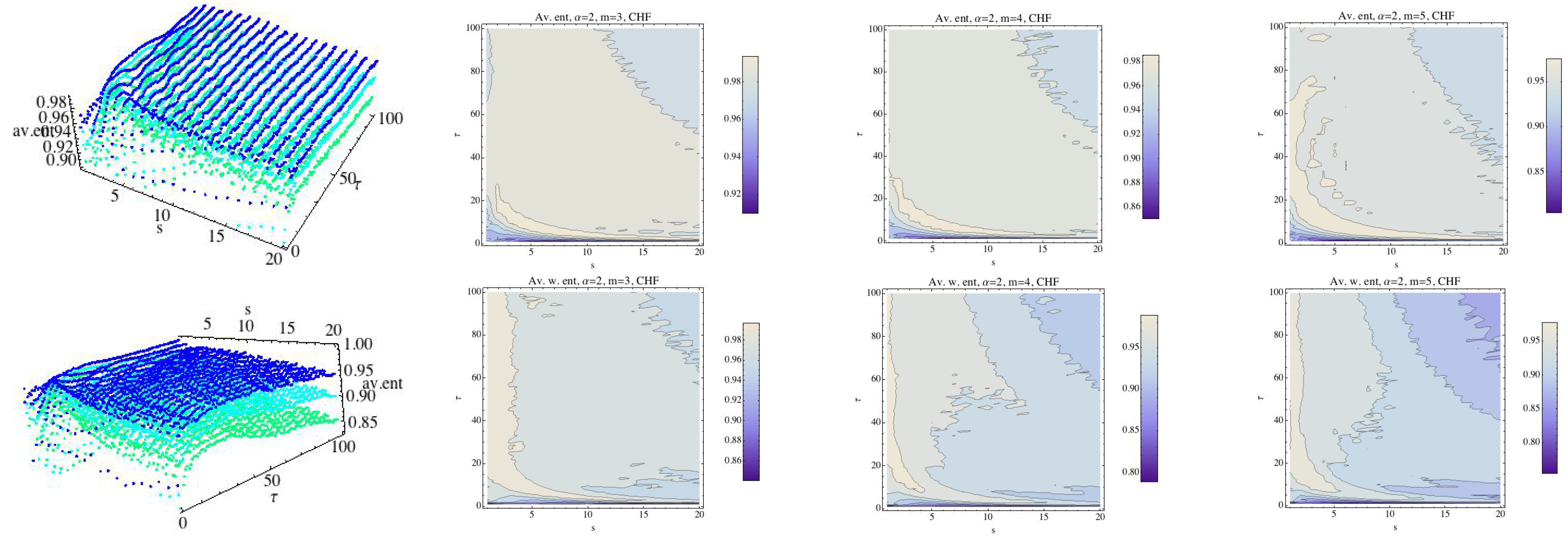
In [13] permutation min-entropy is used to analyze this data collection. Here, we will analyze these series using normalized MRPE and WMRPE entropies. All procedures have been implemented with a code “ad hoc”. First, we analyze the behavior of each group (the mean) for the embedding dimension , , and , taking into account that when the value of m increases, so does the computational time. We fix and as reference values. Regarding the scale factor s, it ranges over the interval and ranges over . The results are shown in Figure 4, Figure 5, Figure 6, Figure 7, Figure 8, Figure 9, Figure 10, Figure 11, Figure 12, Figure 13 and Figure 14. In Figure 4, we have fixed and have computed the average of RPE and WRPE for the CHF group, considering the embedding dimensions (dark blue), (light blue), and (green) in the 3D graph. We can observe in the contour plots that changes in the values of the entropy, that is, changes in the complexity of the dynamics, are presented for values close to the boundary, namely and . When the value of the embedding dimension increases, so does the rate at which the entropy decreases with respect to parameter values and s. We can see that the variability of the values of the entropy for when and s increase is greater when m grows, although the values of the entropy are lower. Finally, for a fixed , changes in the values of the scale parameter s means changes in the values of the RPE and in the values of the WRPE.
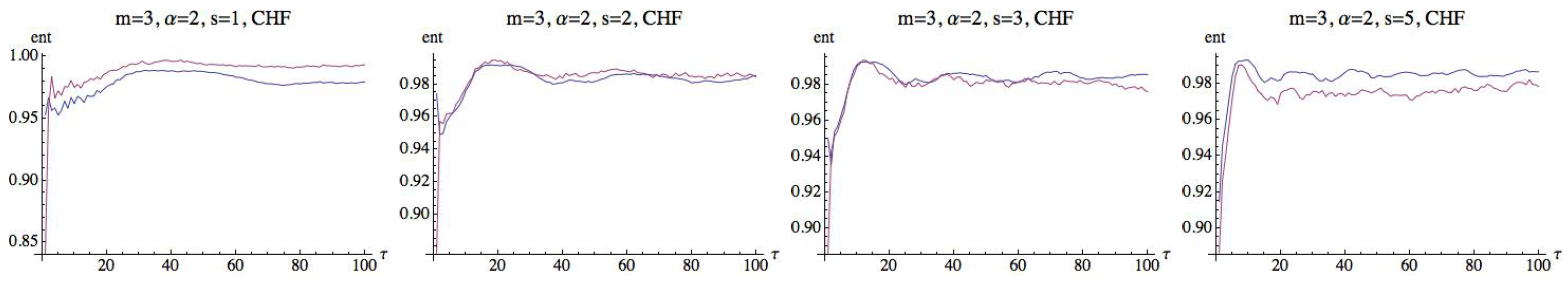
Regarding the relationship between the WRPE and the RPE for a fixed m and , we can observe that it depends on the scale value s; see Figure 5, where the RPE is drawn in blue and the WRPE in red. This relationship can remain unnoticed if multiscale analysis is not involved. Thus, for we can observe that for , the WRPE is greater than or equal to the RPE. Nevertheless, when the order relation changes and there is no rule to determine if an entropy measure is greater than the other one. For values of , the relationship turns around, and the RPE is greater than the WRPE. The limit case and close values of to this gives a different behavior.
Fixing , we compute the average of the RPE and WRPE for the H group. We have drawn RPE in the top row for (dark blue), (light blue), and (green) and the contour plots for each value of the embedding dimension m; see Figure 6. The bottom row shows the results obtained for the WRPE. Again, roughly speaking, as m increases the values of Rényi entropy decreases. We can see that the behavior with respect to the projections for the CHF and H groups are different. Moreover, in the case of the H group, the values of the weighted Rényi entropy are lower than those of the Rényi entropy for most values of , even for the case of , compared to what happened in the case of CHF group; see Figure 7. We recall that the CHF group and the H group were not easy to distinguish. and all the differences must be taken into account.
Finally, we compute the RPE and WRPE for the AF group following the previous schedule. The results are shown in Figure 8, and they are quite different from the results that were obtained for the previous groups. The relationship between the values of RPE and WRPE for are shown in Figure 9. Again, for we can see that there are values of for which the WRPE is greater than the RPE, and the situation changes when s increases. Thus, only the H group has a different behavior in respect to this fact.
The above computations are now made for , and we observe the behavior of each group for this value, which is greater than 1. Results are shown in Figure 10, Figure 11, Figure 12, Figure 13, Figure 14 and Figure 15.
For and there are values of such that the WRPE is greater than the RPE. Figure 11 shows the RPE (blue) and WRPE (red) results for and , , , and .
Following the previous analysis, we have been able to observe some differences between them. Now, we are interested in comparing the groups by analyzing what are the best parameter values to differentiate the three groups. For that, we compute the entropies of each subject and take the maximum and the minimum value in each group for each fixed parameter value. More concretely, fixing the parameter values s, m, , and , we say that two groups are differentiated by the entropy measure if the intervals limited by their corresponding maximum and minimum values are disjoint, and the difference between two groups is the minimum distance between any two values belonging to different groups. Namely, fixing m, , s, and , we compute for a group G
Fixing s, , m, and , we say that group and group are differentiated by the MRPE (resp. WMRPE) if
(resp. ).
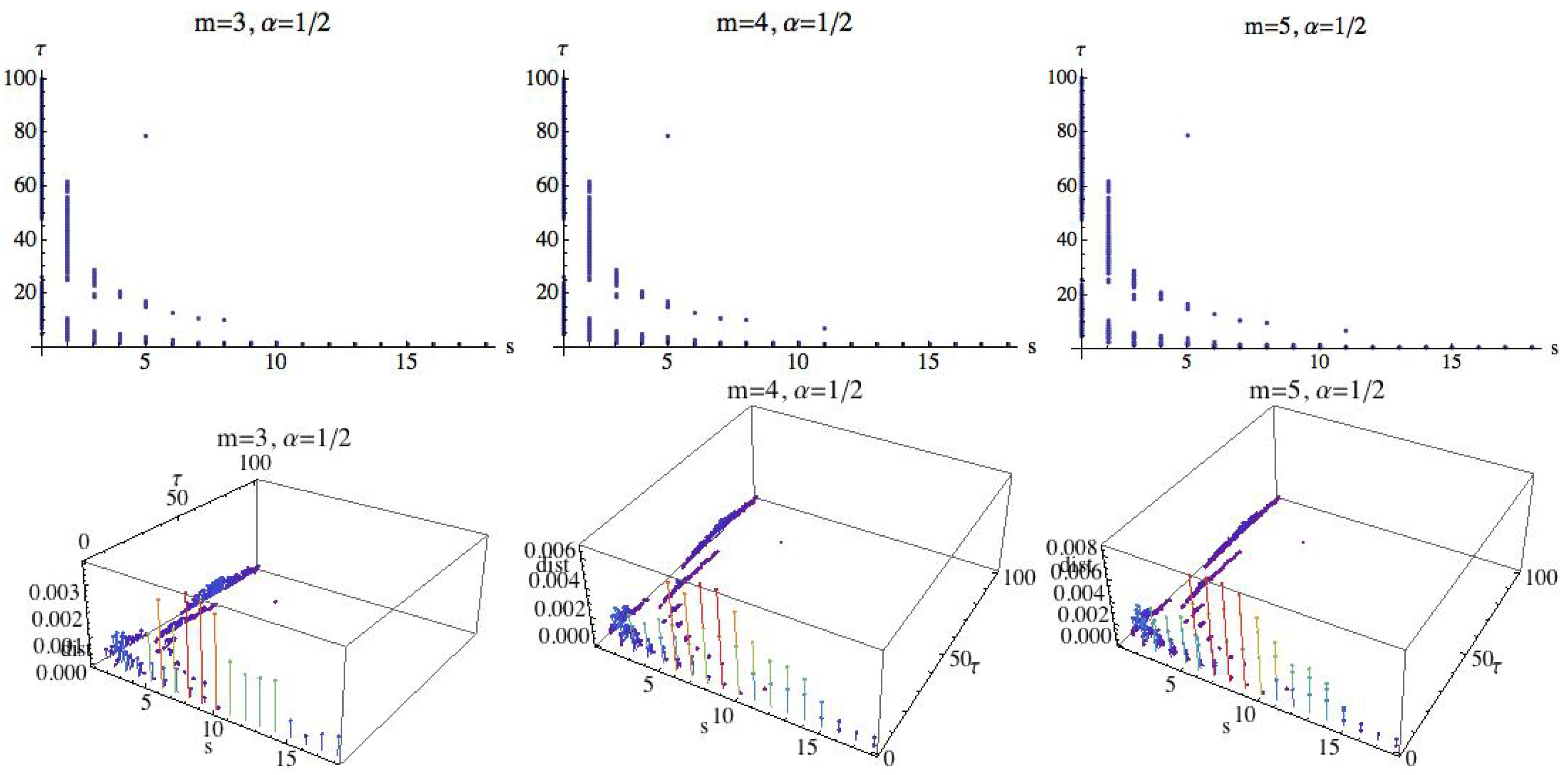
We will investigate the existence of parameter values in which the three groups are differentiated simultaneously. It means that a relationship of order should be given. In addition, in those situations we will compute the difference between and and the difference between and , and we will compute the minimum of both. This value will be called the difference between the three groups. We are interested in finding the parameter values by which the groups are differentiated and the difference is maximal. Observe that although the number of subjects is small, a negative answer to this question also gives valuable information. For this, we fix and consider three different cases: , , and . Figure 16 shows the results for . In 3D graphs (Figure 16), the OX axis represents the parameter s, where , in the OY axis is represented the parameter , , and finally in the OZ axis is represented the difference between the three groups, when the groups are differentiated by MRPE. The 2D graphs show the values for which the three groups are disjoint in the sense described above. Whereas in the 3D plots we can see not only the parameter values in which the three groups are disjoint but also the difference between them. When m changes, the shape of the distribution of the points is similar although the number of points increases, namely for there are 168 points, for there are 283 points, and for there are 348 points. The maximum difference increases with the parameter m, as we can see in Figure 16. The difference attains its maximum values when . The relation of order between the three groups is, in all cases, AF > H > CHF. More details are given in Table 1, where the results for and are shown.
When we compute the WMRPE instead of the MRPE, the results are different. The values that appear in Table 2 show that in general terms, the WMRPE is worse than the MRPE for differentiating the three groups.
Now we consider a fixed value of greater than 1; we follow with the reference value . Figure 17 shows the results. The shape and the distribution of the points for a fixed embedding dimension is similar to the results obtained for , but we can observe that the maximum difference is greater than the one obtained in the above case.
For , when the weighted version is considered, we obtain the points and the differences that have been collected in Table 3, taking , , and .
Following the previous results, we see that the maximum value has been attained for and . To see the influence of the parameter , we set and , and we compute the RPE values in the OY axis for each value of (represented in the OX axis); see Figure 18. We can see that when increases, the entropy values tend to a limit value.
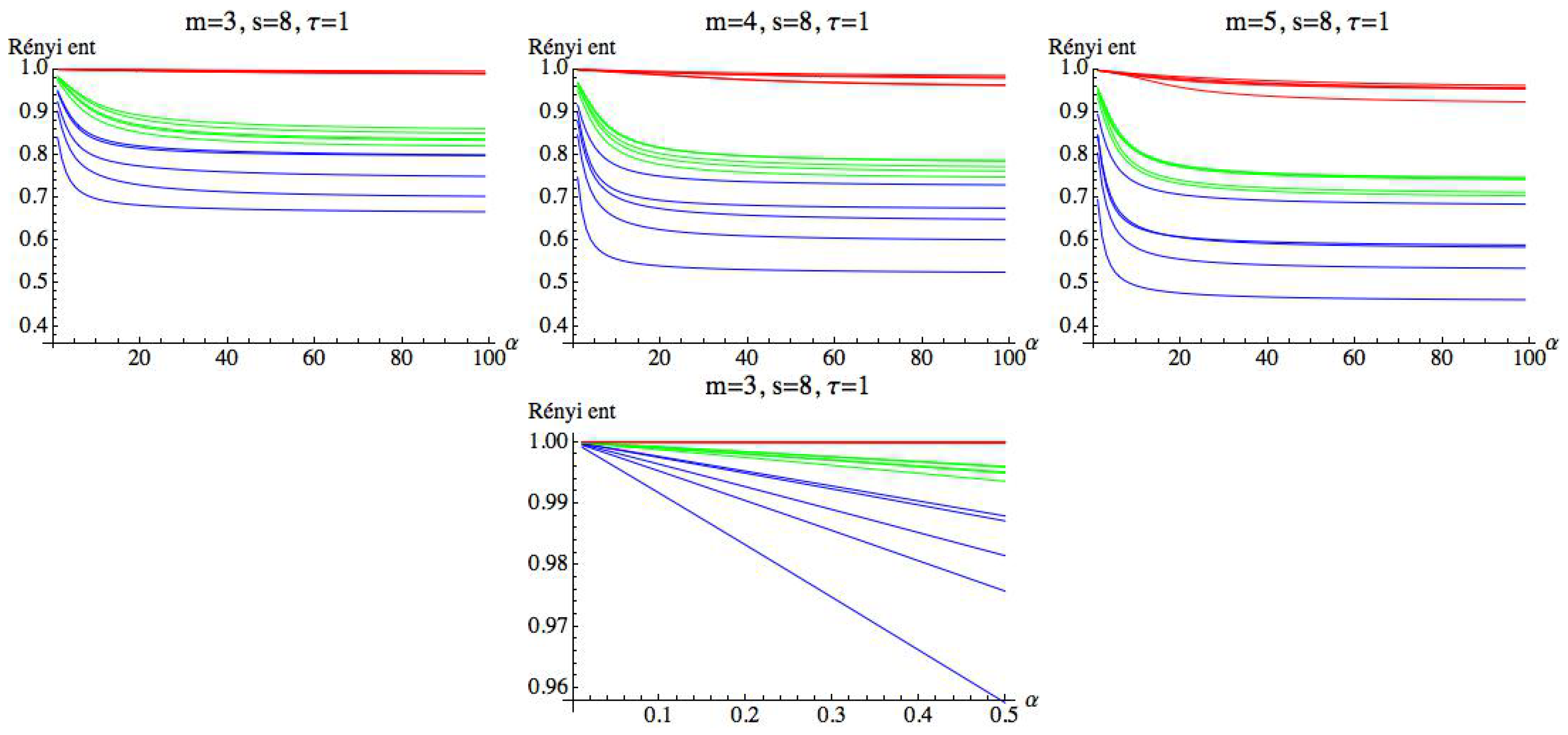
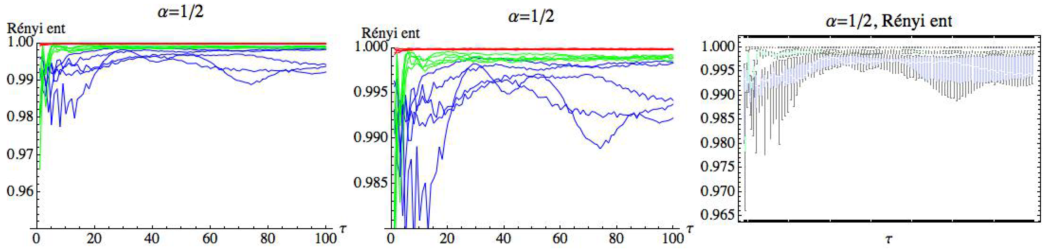
For , we can observe that there is a large quantity of values of for which the three groups are differentiated, although the differences in these values are significantly lower than in the previous case. For , we simply get RPE with delay, , that now runs over a set of cardinality equal to 100. This means that for a fixed m, we have two parameters and . Fixed the embedding dimension , we compute the Rényi entropy for taking values in the interval . Figure 19, Figure 20 and Figure 21 show the results for , , and , respectively. We can see that the AF group has a different behavior from the healthy and CHF groups. It is possible to find values of for which the three groups can be differentiated. More details are included in the Appendix A (Table A1 and Table A2), where different values of have been considered for and . It is observed that when decreases, the entropy values of the different groups are closer.
5. Conclusions
In this paper, we propose a multiscale analysis with RPE and WRPE to analyze heartbeat time series, where four parameters are considered in the study of the behavior of a heartbeat time series. Our purposes are twofold. On the one hand, we have considered the behavior of the entropy measure when parameters change in a range. The introduction of new parameters makes the analysis more difficult and more expensive in computational terms, but on the other hand, when we add new parameters, this allows a better fit to the research objective. From this point of view, it is natural to ask if the introduction of two additional scales gives non-redundant information. In this direction, numerical analysis shows differences between the three groups considered, namely a congestive heart failure (CHF) group, healthy (H) group, and atrial fibrillation (AF) group. Moreover, an additional characteristic for the healthy group is obtained, as we can see that this group has a different behavior in the relationship between the RPE and WRPE when s changes. On the other hand, we compare the results obtained for the RPE and WRPE, and we find the values for which the three groups can be differentiated using segments limited by the minimum and maximum values that have been attained in each group. The groups are called differentiated if the intervals are disjoint. In addition, we compute the values of s and that simultaneously differentiate the three groups, taking the two reference values of and and embedding dimensions and 5. The numerical approach shows that even the RPE is better to differentiate than the WRPE.
The results look promising in the sense that they show that the introduction of multiscale analysis of Rényi entropy reveals more details about the behavior of each group and highlights non-redundant differences between them. The results that have been obtained are a first step in the idea that multiscale analysis should be taken into account to obtain an adequate interpretation of ordinal patterns in physiological terms, in order to consider all of the potential information that they can reveal.
Funding
The author has been supported by the Grant MTM2017-84079-P from Agencia Estatal de Investigación (AEI) y Fondo Europeo de Desarrollo Regional (FEDER).
Acknowledgments
The author thanks anonymous reviewers for their helpful suggestions and comments that have contributed to improving and clarifying this manuscript.
Conflicts of Interest
The author declares no conflict of interest.
Appendix A

Table A1.
PE for and .
| c1rr | c2rr | c3rr | c4rr | c5rr | ||||||
| s | Mean | Mean | Mean | Mean | Mean | |||||
| 1 | ||||||||||
| 25 | ||||||||||
| 50 | ||||||||||
| 75 | ||||||||||
| 100 | ||||||||||
| n1rr | n2rr | n3rr | n4rr | n5rr | ||||||
| s | Mean | Mean | Mean | Mean | Mean | |||||
| 1 | ||||||||||
| 25 | ||||||||||
| 50 | ||||||||||
| 75 | ||||||||||
| 100 | ||||||||||
| a1rr | a2rr | a3rr | a4rr | a5rr | ||||||
| s | Mean | Mean | Mean | Mean | Mean | |||||
| 1 | ||||||||||
| 25 | ||||||||||
| 50 | ||||||||||
| 75 | ||||||||||
| 100 | ||||||||||
Table A2.
Mean and standard deviation for Rényi entropy taking and for different values of .
| Rényi Entropy, | ||||||||||
| Mean | Mean | Mean | Mean | Mean | ||||||
| c1 | 0.99375 | 0.0016742 | 0.995901 | 0.00108809 | 0.997573 | 0.000639407 | 0.998799 | 0.000314675 | 0.999881 | 0.0000310164 |
| c2 | 0.992373 | 0.00440852 | 0.994975 | 0.00288105 | 0.997013 | 0.00170015 | 0.998518 | 0.00083924 | 0.999853 | 0.0000829394 |
| c3 | 0.995505 | 0.00135784 | 0.997034 | 0.000876451 | 0.998235 | 0.000512168 | 0.999123 | 0.000250985 | 0.999913 | 0.0000246431 |
| c4 | 0.997599 | 0.00231847 | 0.998417 | 0.00151459 | 0.999059 | 0.000893696 | 0.999533 | 0.000441177 | 0.999954 | 0.0000436064 |
| c5 | 0.996863 | 0.00300583 | 0.997932 | 0.00197033 | 0.998771 | 0.00116577 | 0.99939 | 0.000576648 | 0.999939 | 0.0000570993 |
| n1 | 0.998866 | 0.00217053 | 0.999249 | 0.00143686 | 0.999552 | 0.000856727 | 0.999777 | 0.000426199 | 0.999978 | 0.0000424152 |
| n2 | 0.998122 | 0.00255504 | 0.99876 | 0.00168197 | 0.999262 | 0.000998495 | 0.999633 | 0.000495129 | 0.999963 | 0.0000491351 |
| n3 | 0.99842 | 0.00220677 | 0.998955 | 0.00145612 | 0.999377 | 0.000865973 | 0.99969 | 0.000429973 | 0.999969 | 0.0000427177 |
| n4 | 0.99882 | 0.00108625 | 0.999219 | 0.000717013 | 0.999535 | 0.000426684 | 0.999768 | 0.000211997 | 0.999977 | 0.000021077 |
| n5 | 0.998207 | 0.00337506 | 0.998817 | 0.00221474 | 0.999296 | 0.00131093 | 0.99965 | 0.000648507 | 0.999965 | 0.0000642098 |
| a1 | 0.999883 | 0.0000746988 | 0.999922 | 0.0000496687 | 0.999953 | 0.0000297382 | 0.999977 | 0.0000148454 | 0.999998 | |
| a2 | 0.99982 | 0.0000692071 | 0.99988 | 0.0000460782 | 0.999928 | 0.0000276183 | 0.999964 | 0.0000137984 | 0.999996 | |
| a3 | 0.999918 | 0.0000260503 | 0.999945 | 0.0000173427 | 0.999967 | 0.0000103941 | 0.999984 | 0.999998 | ||
| a4 | 0.999821 | 0.0000319789 | 0.999881 | 0.0000213546 | 0.999929 | 0.0000128298 | 0.999964 | 0.999996 | ||
| a5 | 0.999809 | 0.0000419525 | 0.999873 | 0.0000279582 | 0.999924 | 0.0000167702 | 0.999962 | 0.999996 | ||
| Mean | Mean | Mean | Mean | Mean | ||||||
| c1 | 0.971488 | 0.00810825 | 0.954373 | 0.0131568 | 0.919262 | 0.022572 | 0.857684 | 0.0325554 | 0.782297 | 0.0321941 |
| c2 | 0.96679 | 0.0200377 | 0.948698 | 0.0309635 | 0.915286 | 0.049456 | 0.864263 | 0.072046 | 0.800394 | 0.0849372 |
| c3 | 0.980388 | 0.00696758 | 0.969188 | 0.0117617 | 0.945976 | 0.0220604 | 0.90024 | 0.0384958 | 0.82708 | 0.0428283 |
| c4 | 0.989489 | 0.0106662 | 0.983489 | 0.0166264 | 0.970898 | 0.0267743 | 0.941862 | 0.0390777 | 0.871617 | 0.0415113 |
| c5 | 0.986294 | 0.0134194 | 0.978577 | 0.0205494 | 0.962802 | 0.0320426 | 0.928468 | 0.0437329 | 0.85563 | 0.0435773 |
| n1 | 0.995255 | 0.00885824 | 0.992754 | 0.0129209 | 0.987708 | 0.0191147 | 0.975157 | 0.0261347 | 0.918917 | 0.0280182 |
| n2 | 0.991919 | 0.0109831 | 0.987451 | 0.0164899 | 0.978208 | 0.0251411 | 0.955622 | 0.0341087 | 0.887612 | 0.0347691 |
| n3 | 0.993263 | 0.00924895 | 0.989563 | 0.0136436 | 0.981805 | 0.0203264 | 0.961995 | 0.0276005 | 0.896366 | 0.0297364 |
| n4 | 0.994969 | 0.00465057 | 0.992169 | 0.00711745 | 0.98615 | 0.011609 | 0.970086 | 0.0179958 | 0.907732 | 0.0205302 |
| n5 | 0.992308 | 0.0144336 | 0.988136 | 0.0209432 | 0.979637 | 0.0296429 | 0.958767 | 0.0378302 | 0.892409 | 0.0385716 |
| a1 | 0.999529 | 0.00030556 | 0.99929 | 0.000464605 | 0.998802 | 0.000792727 | 0.997539 | 0.00164017 | 0.980157 | 0.00615212 |
| a2 | 0.999274 | 0.000280116 | 0.998906 | 0.000423513 | 0.998161 | 0.000716948 | 0.996254 | 0.00148206 | 0.974081 | 0.00573953 |
| a3 | 0.999669 | 0.000105529 | 0.9995 | 0.000159653 | 0.999158 | 0.00027073 | 0.998272 | 0.00056533 | 0.984414 | 0.00439242 |
| a4 | 0.999277 | 0.000126117 | 0.998908 | 0.000187545 | 0.998155 | 0.000307843 | 0.996192 | 0.000600026 | 0.972335 | 0.00283459 |
| a5 | 0.999225 | 0.000168423 | 0.998827 | 0.000253341 | 0.998015 | 0.000424909 | 0.995882 | 0.000865272 | 0.970802 | 0.00409266 |
References
- Bandt, C.; Pompe, B. Permutation entropy, a natural complexity measure for time series. Phys. Rev. Lett. 2002, 88, 174102. [Google Scholar] [CrossRef] [PubMed]
- Zanin, M.; Zunino, L.; Rosso, O.A.; Papo, D. Permutation Entropy and its Main Biomedical and Econophysics Applications: A Review. Entropy 2012, 14, 1553–1577. [Google Scholar] [CrossRef]
- Amigó, J.M.; Keller, K.; Unakafova, V.A. Ordinal symbolic analysis and its applications to biomedical recordings. Phil. Trans. R. Soc. A 2015, 373, 20170091. [Google Scholar] [CrossRef] [PubMed]
- Keller, K.; Mangold, T.; Stolz, I.; Werner, J. Permutation entropy: New ideas and challenges. Entropy 2017, 19, 134. [Google Scholar] [CrossRef]
- Pincus, S.M.; Gladstone, I.M.; Ehrenkranz, R.A. A regularity statistic for medical data analysis. J. Clin. Monit. 1991, 7, 335–345. [Google Scholar] [CrossRef]
- Pincus, S.M.; Goldberger, A.L. Physiological time-series analysis: What does regularity quantify? Am. J. Physiol. 1994, 266, 1643–1656. [Google Scholar] [CrossRef]
- Kurths, J.; Voss, A.; Saparin, P.; Witt, A.; Kleiner, H.J.; Wessel, N. Quantitative analysis of heart rate variability. Chaos 1995, 5, 88–94. [Google Scholar] [CrossRef]
- Lake, D.E.; Richman, J.S.; Griffin, M.P.; Moorman, J.R. Sample entropy analysis of neonatal heart rate variability. Am. J. Physiol. Regul. Integr. Comp. Physiol. 2002, 283, R789–R797. [Google Scholar] [CrossRef] [Green Version]
- Zeng, W.; Glass, L. Statistical properties of heartbeat intervals during atrial fibrillation. Phys. Rev. E 1996, 52, 1779–1784. [Google Scholar] [CrossRef]
- Cammarota, C.; Rogora, E. Independence and symbolic independence of nonstationary heartbeat series during atrial fibrillation. Phys. A 2005, 353, 323–335. [Google Scholar] [CrossRef]
- Porta, A.; Guzzetti, S.; Montano, N.; Furlan, R.; Pagani, R.; Malliani, A.; Cerutti, S. Entropy, Entropy Rate, and Pattern Classification as tools to typify complexity in short heart period variability series. IEEE Trans. Biomed. Eng. 2001, 48, 1282–1291. [Google Scholar] [CrossRef] [PubMed]
- Graff, B. Entropy measures of heart rate variability for short ECG datasets in patients with congestive heart failure. Acta Phys. Pol. B Proc. Suppl. 2012, 5, 153–158. [Google Scholar] [CrossRef]
- Zunino, L.; Olivares, F.; Rosso, O.A. Permutation min-entropy: An improved quantifier for unveiling subtle temporal correlations. EPL 2015, 109, 10005. [Google Scholar] [CrossRef]
- Xia, Y.; Yang, L.; Zunino, L.; Shi, H.; Zhuang, Y.; Liu, C. Application of Permutation Entropy and Permutation Min-Entropy in Multiple Emotional States Analysis of RRI Times Series. Entropy 2018, 20, 148. [Google Scholar] [CrossRef]
- Costa, M.; Goldberger, A.L.; Peng, C.K. Multiscale Entropy Analysis of Complex Physiologic Time Series. Phys. Rev. Lett. 2002, 89, 068102. [Google Scholar] [CrossRef] [PubMed]
- Liang, Z.; Wang, Y.; Sun, X.; Li, D.; Voss, L.J.; Sleigh, J.W.; Hagihira, S.; Li, X. EEG entropy measures in anesthesia. Front. Comput. Neurosci. 2015, 9, 00016. [Google Scholar] [CrossRef] [PubMed]
- Chen, S.; Shang, P.; Wu, Y. Weighted multiscale Rényi permutation entropy of nonlinear time series. Phys. A 2018, 496, 548–570. [Google Scholar] [CrossRef]
- Cánovas, J.S.; Guillamón, A.; Ruíz, M.C. Using permutations to detect dependence between time series. Phys. D Nonlinear Phenom. 2011, 240, 1199–1204. [Google Scholar] [CrossRef]
- Cánovas, J.S.; García-Clemente, G.; Muñoz-Guillermo, M. Comparing permutation entropy functions to detect structural changes in times series. Phys. A 2018, 507, 153–174. [Google Scholar] [CrossRef]
- Amigó, J.M.; Zambrano, S.; Sanjuán, M.A.F. Combinatorial detection of determinism in noisy time series. EPL 2008, 83, 60005. [Google Scholar] [CrossRef]
- Rényi, A. On measures of entropy and information. Proc. Fourth Berkeley Symp. Math. Stat. Probab. 1961, 1, 547–561. [Google Scholar]
- Zunino, L.; Pérez, D.G.; Kowalski, A.; Martín, M.T.; Caravaglia, M.; Plastino, A.; Rosso, O.A. Brownian motion, fractional Gaussian noise and Tsallis permutation entropy. Phys. A 2008, 387, 6057–6068. [Google Scholar] [CrossRef]
- Tsallis, C. Generalized entropy-based criterion for consistent testing. Phys. Rev. E 1998, 58, 1442–1445. [Google Scholar] [CrossRef]
- Versaci, M.; La Foresta, F.; Morabito, F.C.; Angiulli, G. A fuzzy divergence approach for solving electrostatic identification problems for NDT applications. Int. J. Appl. Electrom. 2018, 57, 133–146. [Google Scholar] [CrossRef]
Figure 1.
The ordinal pattern is represented by two different vectors, (left) and (right). The distance between the values is clearly different.
Figure 1.
The ordinal pattern is represented by two different vectors, (left) and (right). The distance between the values is clearly different.

Figure 2.
Heart beat interval series n1 (left), a1 (middle), and c1 (right). In each figure, heart beat (RR) intervals (in seconds) are plotted.
Figure 2.
Heart beat interval series n1 (left), a1 (middle), and c1 (right). In each figure, heart beat (RR) intervals (in seconds) are plotted.

Figure 3.
In the left, the permutation entropy (PE) for and is represented for each subject. The blue color represents the congestive heart failure (CHF) group, green has been used for the healthy (H) group, and red for the atrial fibrillation (AF) group. The delay parameter has been represented in the axis. In the middle, the same situation has been represented using box plots, grouping the subjects belonging to the same group. Finally, in the right, we have taken the mean with respect to when for each subject and have represented the corresponding box plot.

Figure 4.
Average of Rényi entropy and average weighted Rényi entropy for the CHF group and . We have fixed (dark blue), (light blue), and (green). The top row is for the Rényi permutation entropy (RPE) and the bottom one for the weighted Rényi entropy (WRPE). The projection of the values (contour plot) of the entropy for each fixed embedding dimension for the CHF group have been drawn in 2D graphs.

Figure 5.
Average Rényi entropy (RPE) (blue) and average weighted Rényi entropy (WRPE) (red) for the CHF group with , , and , and 5. Observe that for , the WRPE is higher than the RPE for most values of . Nevertheless, for the situation changes.
Figure 5.
Average Rényi entropy (RPE) (blue) and average weighted Rényi entropy (WRPE) (red) for the CHF group with , , and , and 5. Observe that for , the WRPE is higher than the RPE for most values of . Nevertheless, for the situation changes.

Figure 6.
Average Rényi entropy in the top row and average weighted Rényi entropy in the bottom row for the H group and . We have fixed (dark blue), (light blue), and (green). The projections of the entropy for each fixed embedding dimension for the H group have been drawn in 2D graphs.
Figure 6.
Average Rényi entropy in the top row and average weighted Rényi entropy in the bottom row for the H group and . We have fixed (dark blue), (light blue), and (green). The projections of the entropy for each fixed embedding dimension for the H group have been drawn in 2D graphs.

Figure 7.
Average Rényi entropy (blue) and average weighted Rényi entropy (red) for the H group and , , and , and 5.
Figure 7.
Average Rényi entropy (blue) and average weighted Rényi entropy (red) for the H group and , , and , and 5.

Figure 8.
Average Rényi entropy in the top row and average weighted Rényi entropy in the bottom row for the AF group and . We have fixed (dark blue), (light blue), and (green). The contour of the entropy for each fixed embedding dimension for the AF group has been drawn In 2D graphs.
Figure 8.
Average Rényi entropy in the top row and average weighted Rényi entropy in the bottom row for the AF group and . We have fixed (dark blue), (light blue), and (green). The contour of the entropy for each fixed embedding dimension for the AF group has been drawn In 2D graphs.

Figure 9.
Average Rényi entropy (RPE) (blue) and average weighted Rényi entropy (WRPE) (red) for the AF group and , , and , and 5.
Figure 9.
Average Rényi entropy (RPE) (blue) and average weighted Rényi entropy (WRPE) (red) for the AF group and , , and , and 5.

Figure 10.
Average Rényi entropy in the top row and average weighted Rényi entropy in the bottom row for the CHF group and . We have fixed (dark blue), (light blue), and (green). The projections of the entropy for each fixed embedding dimension for the CHF group have been drawn in 2D graphs.
Figure 10.
Average Rényi entropy in the top row and average weighted Rényi entropy in the bottom row for the CHF group and . We have fixed (dark blue), (light blue), and (green). The projections of the entropy for each fixed embedding dimension for the CHF group have been drawn in 2D graphs.

Figure 11.
Average Rényi entropy (RPE, blue) and average weighted Rényi entropy (WRPE, red) for the CHF group and , , and , and 5. Observe that for , the WRPE is higher for most values of ; nevertheless, for the situation changes.
Figure 11.
Average Rényi entropy (RPE, blue) and average weighted Rényi entropy (WRPE, red) for the CHF group and , , and , and 5. Observe that for , the WRPE is higher for most values of ; nevertheless, for the situation changes.

Figure 12.
Average Rényi entropy and average weighted Rényi entropy for the H group and . We have fixed (dark blue), (light blue), and (green). The projections of the entropy for each fixed embedding dimension for the H group have been drawn in 2D graphs.
Figure 12.
Average Rényi entropy and average weighted Rényi entropy for the H group and . We have fixed (dark blue), (light blue), and (green). The projections of the entropy for each fixed embedding dimension for the H group have been drawn in 2D graphs.

Figure 13.
Average Rényi entropy (RPE, blue) and average weighted Rényi entropy (WRPE, red) for the H group and , , and , and 5.
Figure 13.
Average Rényi entropy (RPE, blue) and average weighted Rényi entropy (WRPE, red) for the H group and , , and , and 5.

Figure 14.
Average Rényi entropy in the top row and average weighted Rényi entropy in the bottom row for the AF group and . We have fixed (dark blue), (light blue), and (green). The contour plots of the entropy for each fixed embedding dimension for the AF group have been drawn in 2D graphs.
Figure 14.
Average Rényi entropy in the top row and average weighted Rényi entropy in the bottom row for the AF group and . We have fixed (dark blue), (light blue), and (green). The contour plots of the entropy for each fixed embedding dimension for the AF group have been drawn in 2D graphs.

Figure 15.
Average of Rényi entropy (RPE, blue) and average of weighted Rényi entropy (WRPE, red) for the AF group and , , and , and 5.
Figure 15.
Average of Rényi entropy (RPE, blue) and average of weighted Rényi entropy (WRPE, red) for the AF group and , , and , and 5.

Figure 16.
For , values of s and for which the three groups are separated by the multiscale Rényi permutation entropy (MRPE). In the 3D graphs, the OX axis represents the parameter s, where , in the OY axis is represented the parameter , , and finally in the OZ axis is represented the difference between the three groups, when the groups are differentiated by the MRPE.

Figure 17.
Fixing , values of s and for which the three groups are separated by the MRPE are shown. In the 3D graphs, the OX axis represents the parameter s, where , in the OY axis is represented the parameter , , and finally in the OZ axis is represented the difference between the three groups, when the groups are differentiated by the MRPE.

Figure 18.
The top row shows the RPE for , and (left), (middle), and (right). In red is the AF group, in green is the H group, and the CHF results are in blue. The OX axis represents . and the RPE is represented in the OY axis. The bottom graph shows the results for , , and for .
Figure 18.
The top row shows the RPE for , and (left), (middle), and (right). In red is the AF group, in green is the H group, and the CHF results are in blue. The OX axis represents . and the RPE is represented in the OY axis. The bottom graph shows the results for , , and for .

Figure 19.
Rényi entropy for and embedding dimension . We have drawn the Rényi entropy for the CHF group in blue, for the healthy group in green, and for the AF group in red, on the left. A zoomed-in view of the right figure is shown in the middle, where the differences between the three groups when runs over the range can be appreciated. Finally, box plots for each group have been represented on the right.

Figure 20.
Rényi entropy for and embedding dimension . We have drawn the Rényi entropy for the CHF group in blue, for the healthy group in green, and for the AF group in red on the left.
Figure 20.
Rényi entropy for and embedding dimension . We have drawn the Rényi entropy for the CHF group in blue, for the healthy group in green, and for the AF group in red on the left.

Figure 21.
Rényi entropy for and embedding dimension . We have drawn the Rényi entropy for the CHF group in blue, for the healthy group in green, and for the AF group in red on the left. A zoomed-in view of the right figure is shown in the middle, where the differences between the three groups when runs over the range can be appreciated. Finally, box plots for each group have been represented on the right.

Table 1.
For and , values of s and for which the three groups are disjoint.
| s | |
|---|---|
| 1 | 5, 7, 8, 9, 10, 11, 12, 13, 14, 15, 16, 17, 18, 19, 20, 21, 22, 23, 24, 26, 48, 49, 50, 51, 52, 53, 54, 55, 56, 57, 58, 59, 60, 61, 62, 63, 64, 65, 66, 67, 68, 69, 70, 71, 72, 73, 74, 75, 76, 77, 78, 79, 80, 81, 82, 83, 84, 85, 86, 87, 88, 89, 90, 91, 92, 93, 94, 95, 96, 97, 98, 99, 100 |
| 2 | 3, 4, 5, 6, 7, 8, 9, 10, 11, 25, 26, 28, 29, 30, 31, 32, 33, 34, 35, 36, 37, 38, 39, 40, 41, 42, 43, 44, 45, 46, 47, 48, 49, 50, 51, 52, 53, 54, 55, 56, 58, 59, 60, 61, 62 |
| 3 | 2, 3, 4, 5, 6, 19, 20, 23, 24, 25, 26, 27, 28, 29 |
| 4 | 2, 3, 4, 5, 19, 20, 21 |
| 5 | 2, 3, 4, 15, 16, 17, 79 |
| 6 | 1, 2, 3, 13 |
| 7 | 1, 2, 11 |
| 8 | 1, 2, 10 |
| 9 | 1, 2 |
| 10 | 1, 2 |
| 11 | 1 |
| 12 | 1 |
| 13 | 1 |
| 14 | 1 |
| 15 | 1 |
| 16 | 1 |
| 17 | 1 |
| 18 | 1 |
Table 2.
Fixing , values for the parameters in the ranges , , and such that the CHF group, H group, and AF group are disjoint. The difference is included, as well as the order relation between them.
Table 2.
Fixing , values for the parameters in the ranges , , and such that the CHF group, H group, and AF group are disjoint. The difference is included, as well as the order relation between them.
| m | s | Difference | Relation | |
|---|---|---|---|---|
| 3 | 1 | 3 | 0.000111612 | |
| 4 | 1 | 3 | 0.000111612 | |
| 5 | 1 | 3 | 0.000111612 | |
| 5 | 11 | 1 | 0.0018635 | |
| 5 | 6 | 2 | 0.00249138 |
Table 3.
Fixing , values for the parameters in the ranges , , and such that the CHF group, H group, and AF group are disjoint. The difference and the order relation between them are also included.
Table 3.
Fixing , values for the parameters in the ranges , , and such that the CHF group, H group, and AF group are disjoint. The difference and the order relation between them are also included.
| m | s | Difference | Relation | |
|---|---|---|---|---|
| 3 | 1 | 3 | 0.000435339 | |
| 4 | 11 | 1 | 0.00213423 | |
| 4 | 6 | 2 | 0.00461844 | |
| 4 | 1 | 3 | 0.000435339 | |
| 5 | 11 | 1 | 0.00213423 | |
| 5 | 6 | 2 | 0.00461844 | |
| 5 | 9 | 1 | 0.0105166 | |
| 5 | 10 | 1 | 0.00585264 | |
| 5 | 5 | 2 | 0.00935592 | |
| 5 | 1 | 3 | 0.000435339 |
© 2019 by the author. Licensee MDPI, Basel, Switzerland. This article is an open access article distributed under the terms and conditions of the Creative Commons Attribution (CC BY) license (http://creativecommons.org/licenses/by/4.0/).
Share and Cite
MDPI and ACS Style
Muñoz-Guillermo, M. Ordinal Patterns in Heartbeat Time Series: An Approach Using Multiscale Analysis. Entropy 2019, 21, 583. https://doi.org/10.3390/e21060583
AMA Style
Muñoz-Guillermo M. Ordinal Patterns in Heartbeat Time Series: An Approach Using Multiscale Analysis. Entropy. 2019; 21(6):583. https://doi.org/10.3390/e21060583
Chicago/Turabian StyleMuñoz-Guillermo, María. 2019. "Ordinal Patterns in Heartbeat Time Series: An Approach Using Multiscale Analysis" Entropy 21, no. 6: 583. https://doi.org/10.3390/e21060583
Note that from the first issue of 2016, this journal uses article numbers instead of page numbers. See further details here.