Small Order Patterns in Big Time Series: A Practical Guide

Abstract
1. Order Patterns Fit Big Data
1.1. The Need for New Methods
- Basic methods should be simple and transparent.
- Few assumptions should be made on the underlying process.
- Algorithms should be resilient with respect to outliers and artifacts.
- Computations should be very fast.
1.2. Contents of the Paper
1.3. A Typical Example
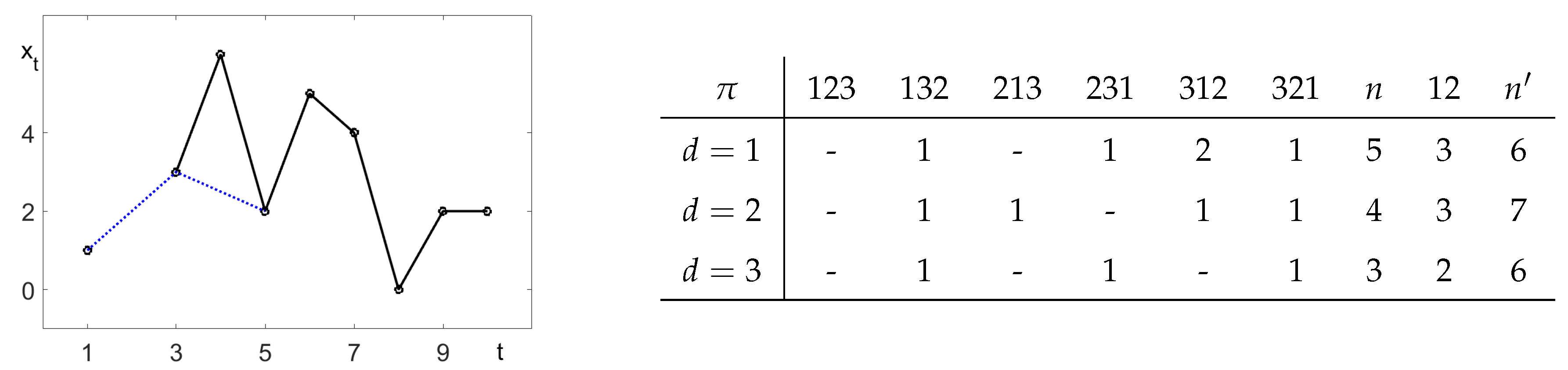
2. Pattern Frequencies
2.1. Basic Idea
2.2. Stationarity
2.3. Calculation of Pattern Frequencies
3. Key Concepts and Viewpoints
3.1. Permutation Entropy and
3.2. Order Correlation Functions
3.3. Relative Order Correlation Functions
3.4. Two Types of Data
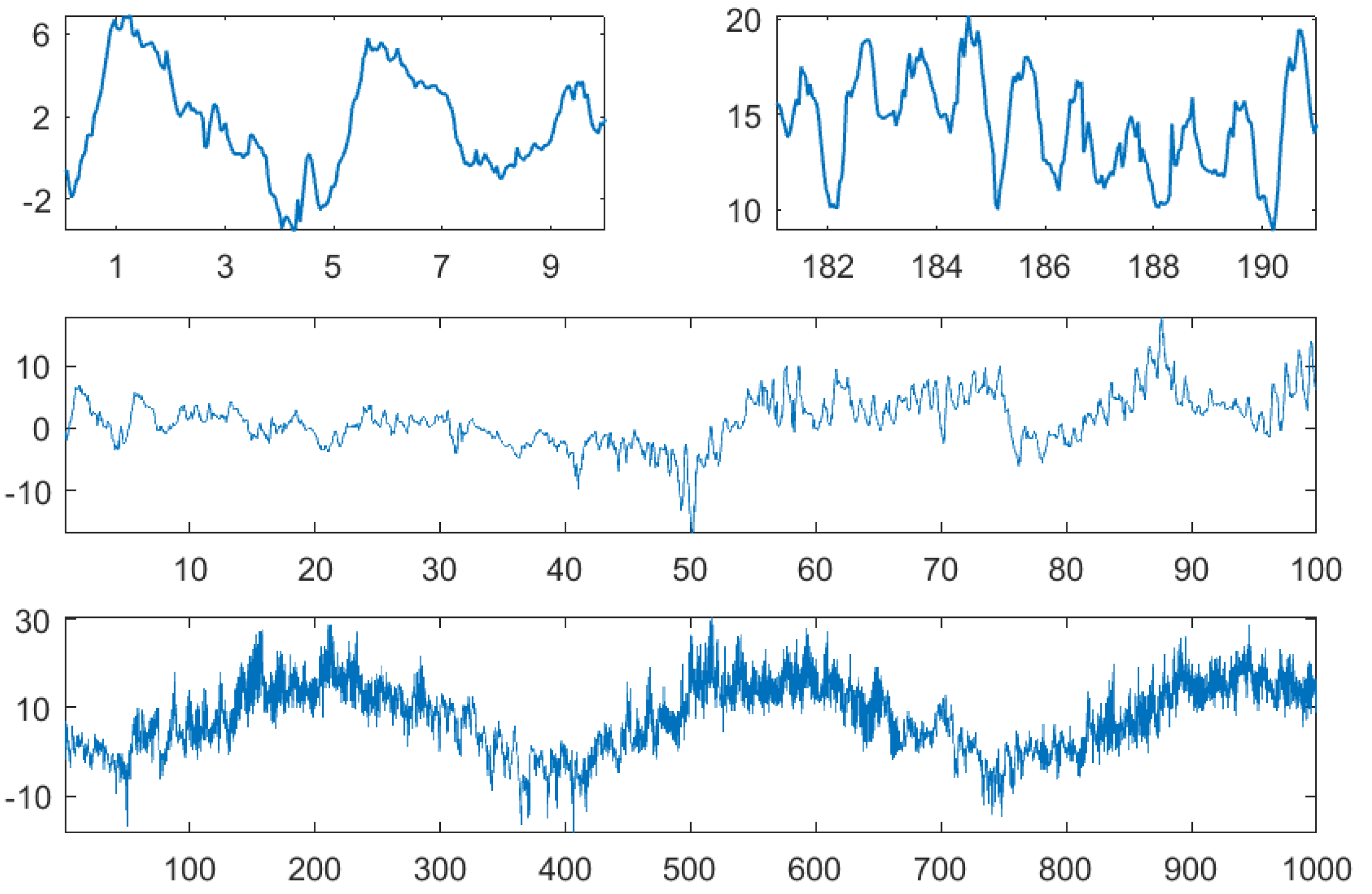
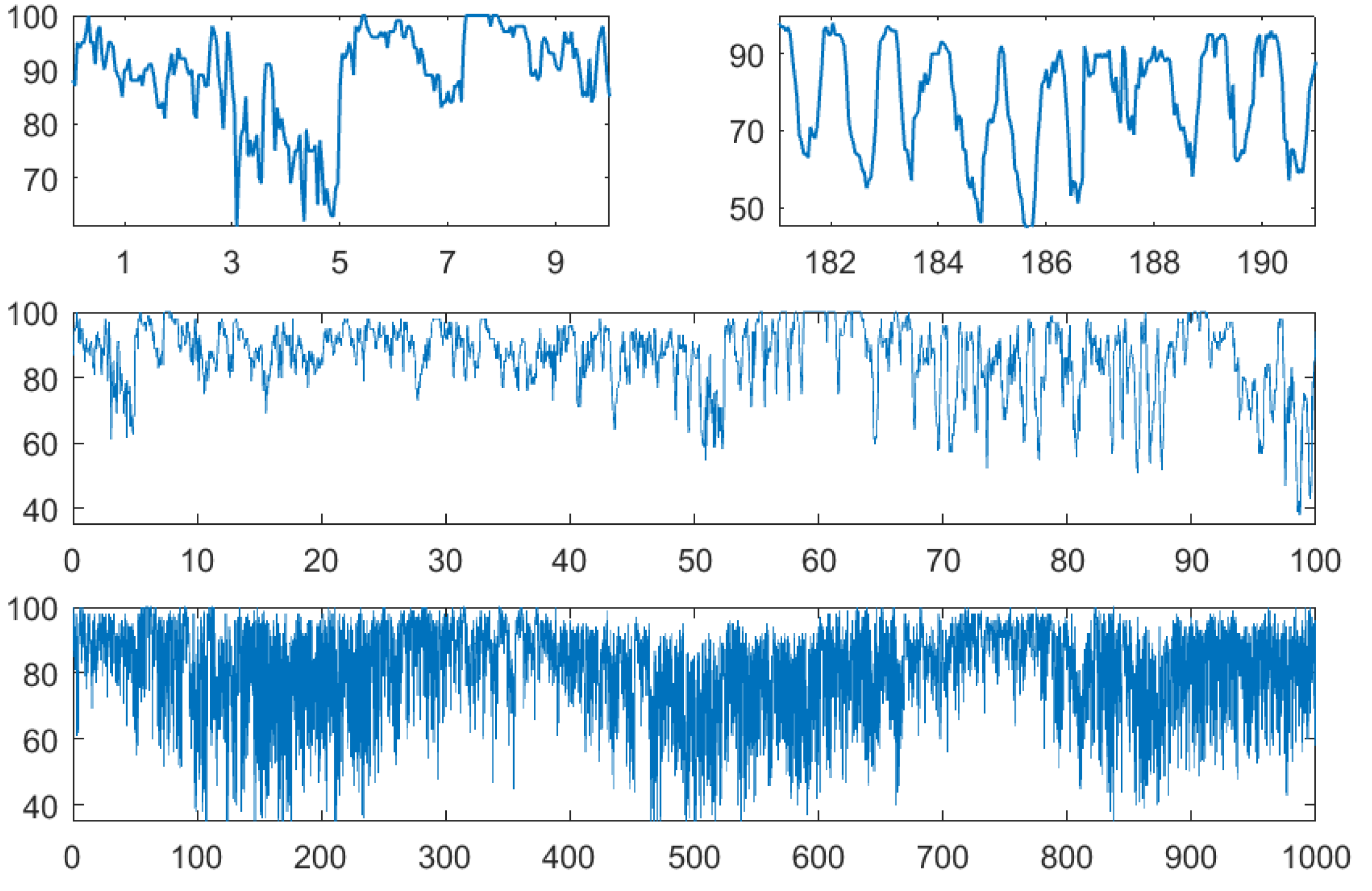
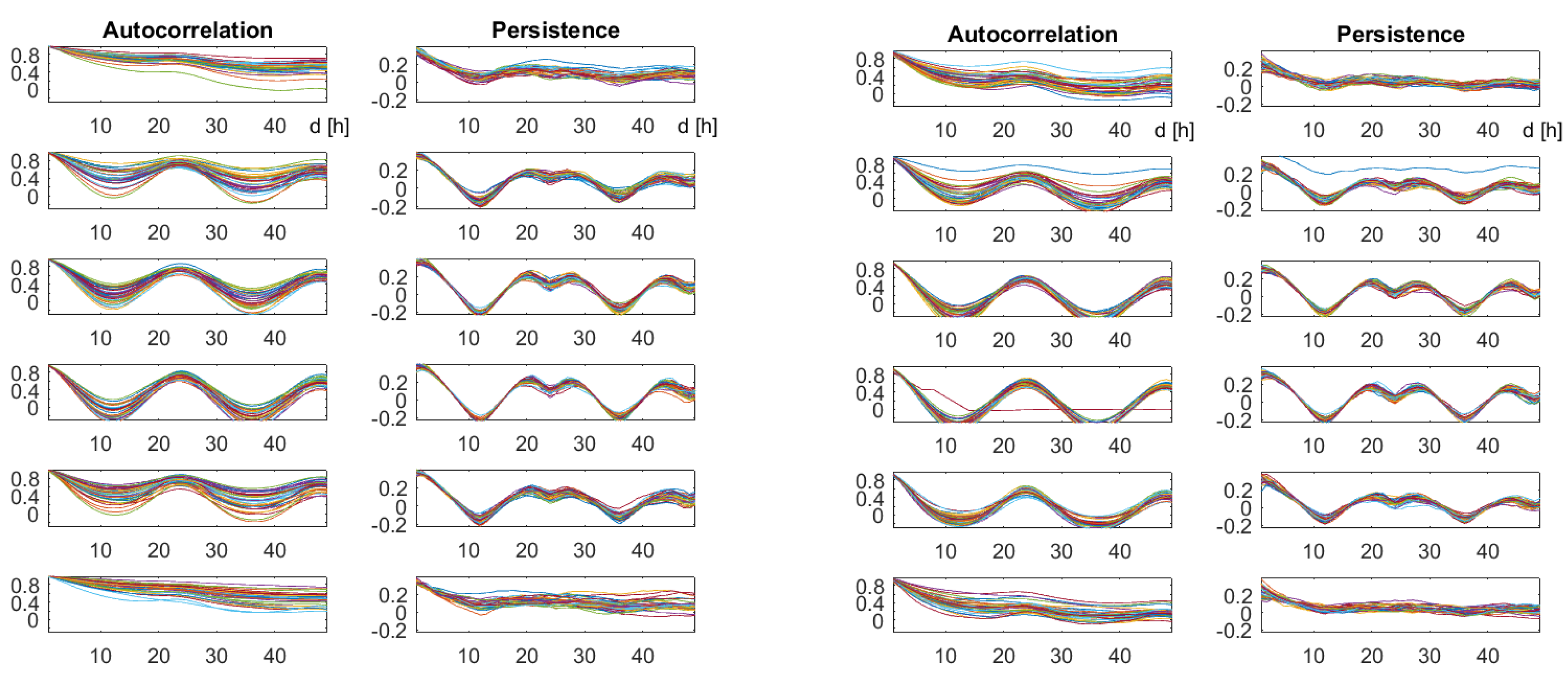
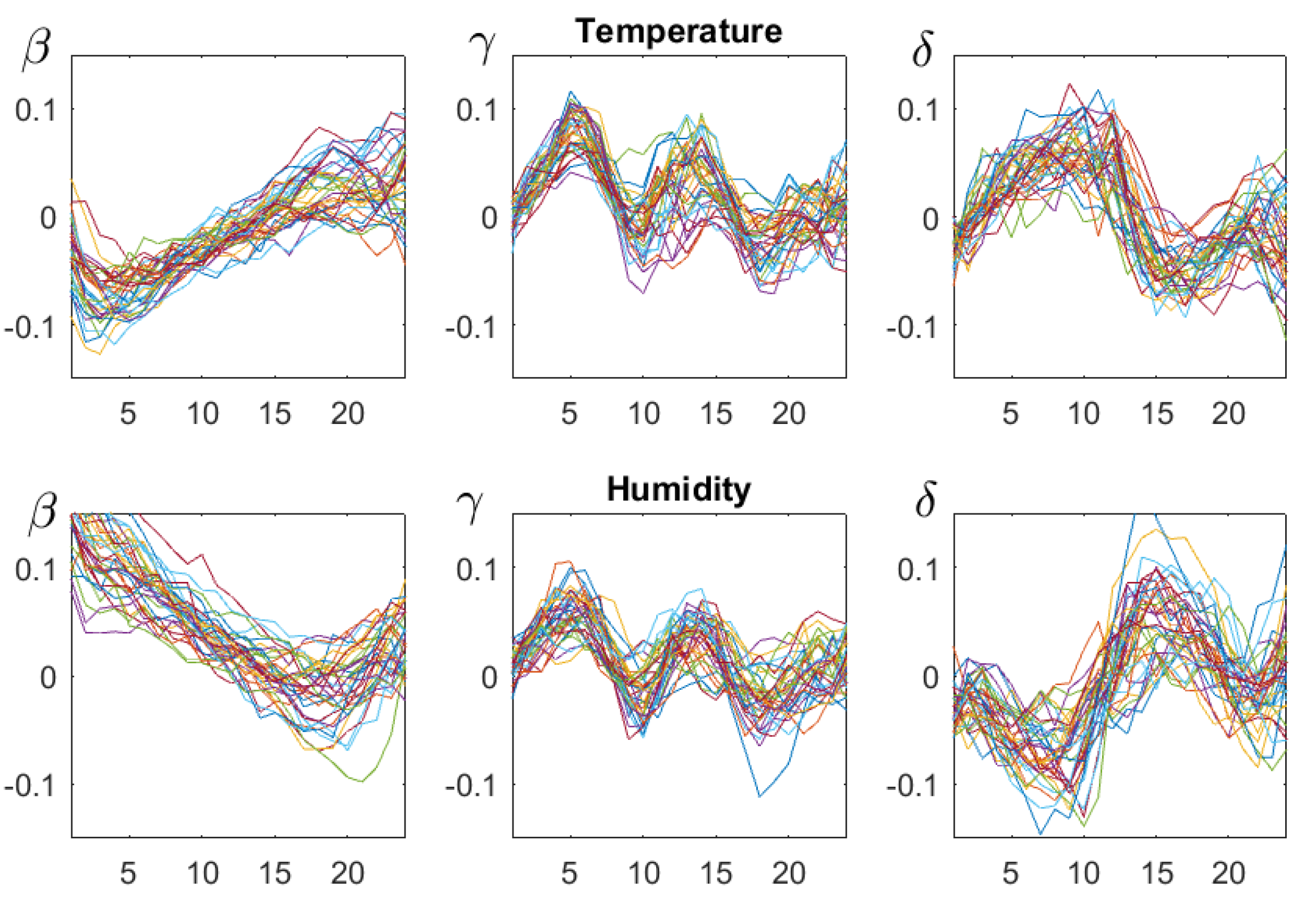
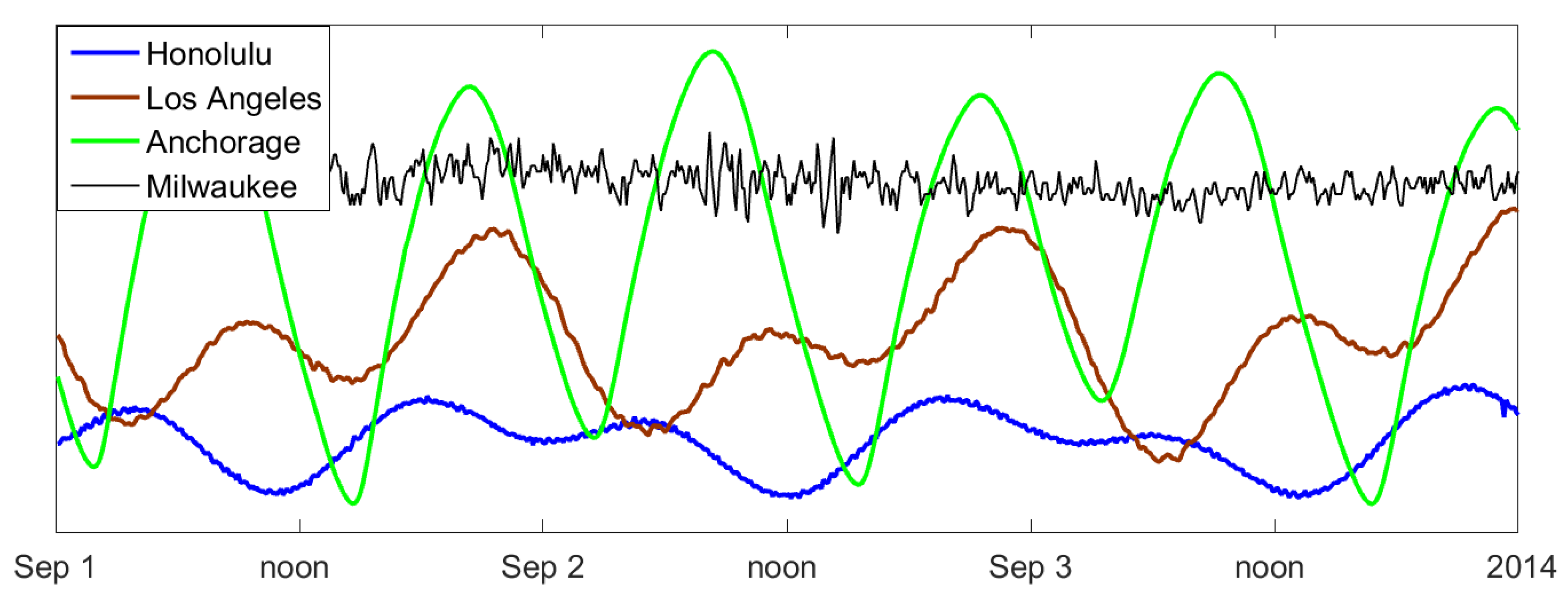
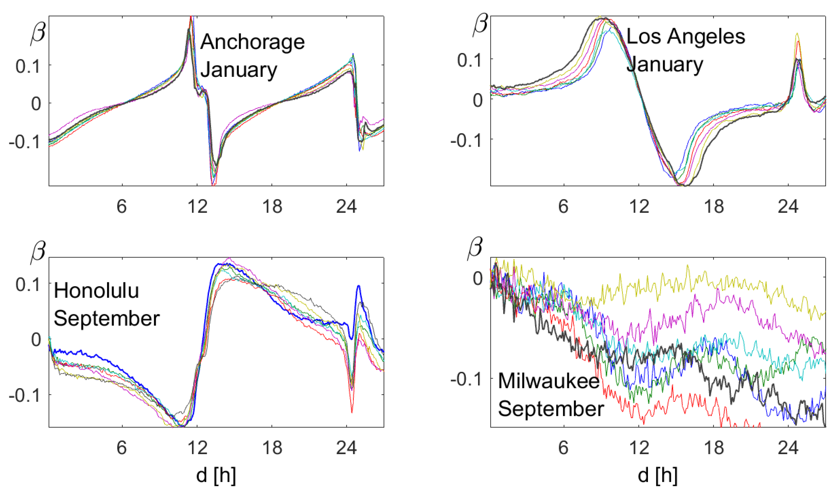
4. First Examples: Weather Data
4.1. The Data
4.2. Autocorrelation and Persistence
4.3. and
5. Properties of Correlation Functions
5.1. Two Pattern Identities
5.2. Marginal Errors
5.3. Classical Autocorrelation
5.4. Interpretation of
5.5. Persistence and Turning Rate
5.6. Symmetries of Order Functions
5.7. Periodicities
5.8. The Decomposition Theorem
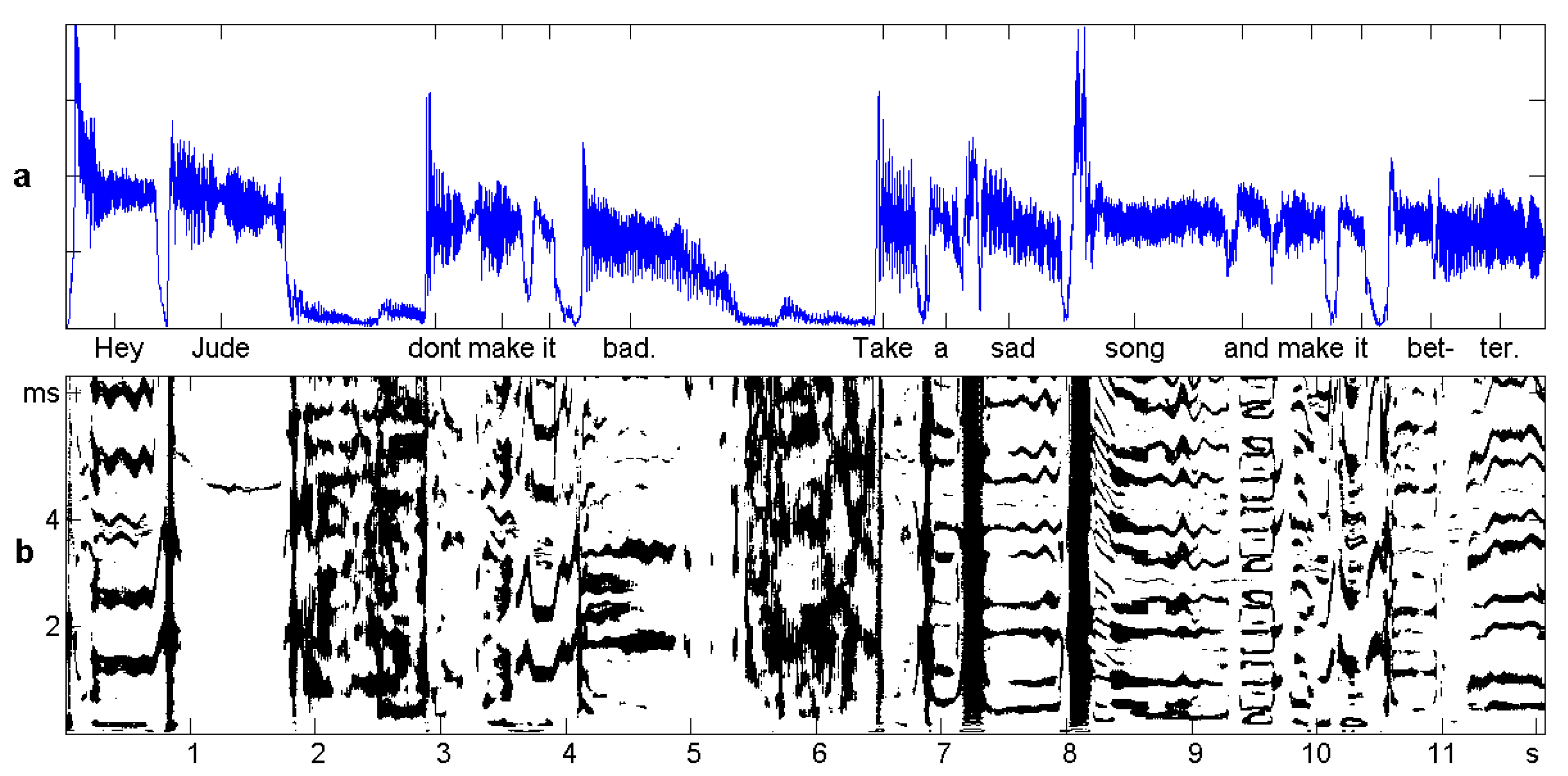
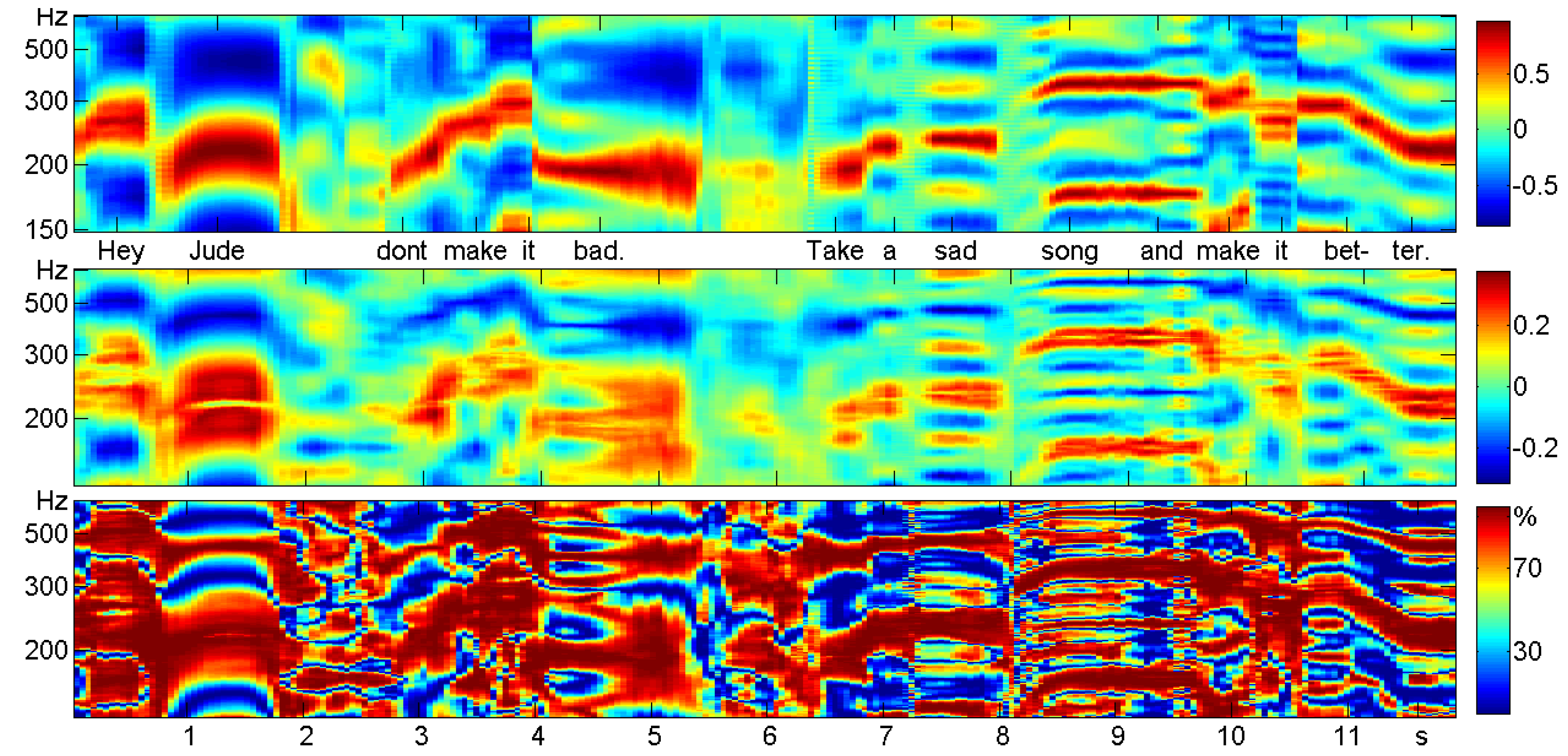
6. Case Study: Speech and Music
Sliding Windows
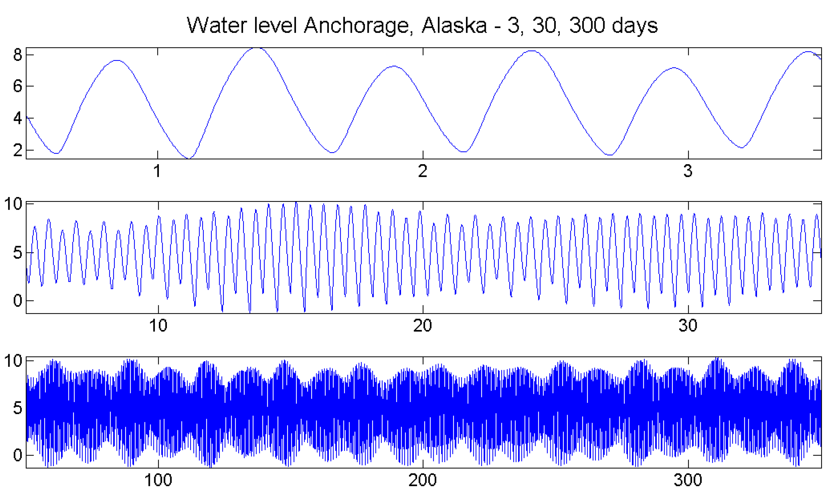
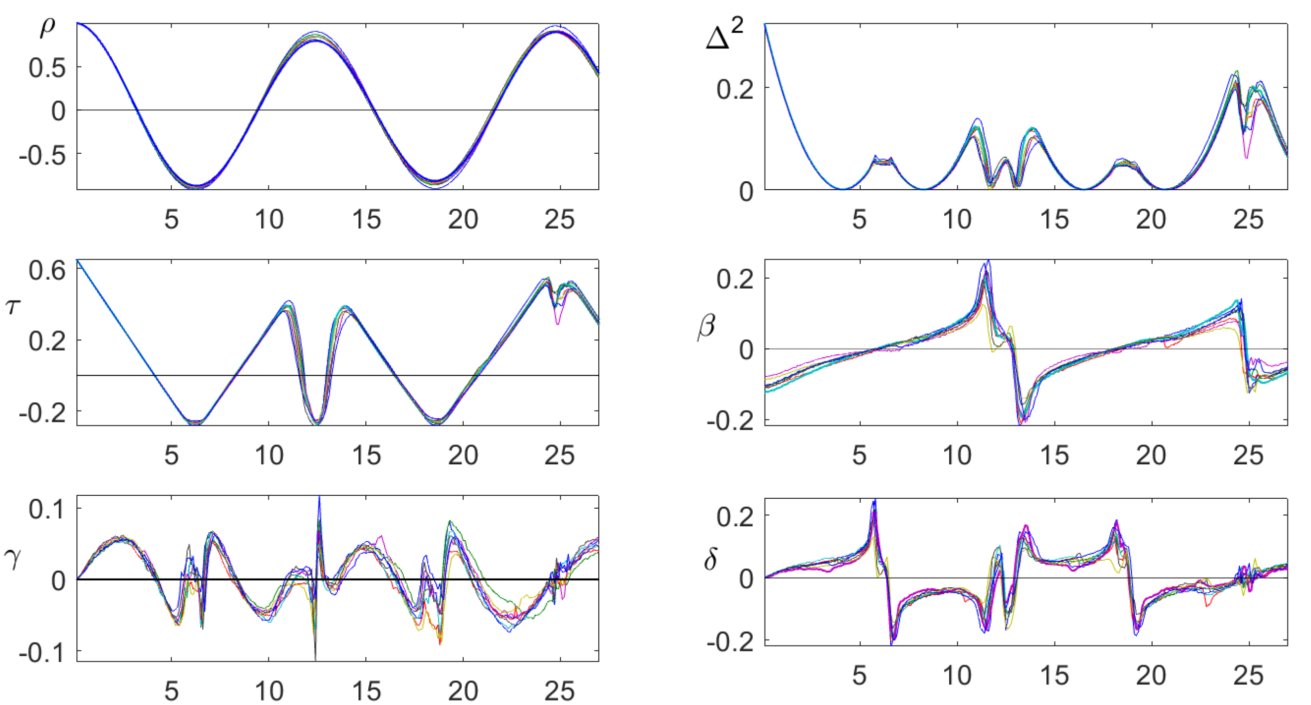
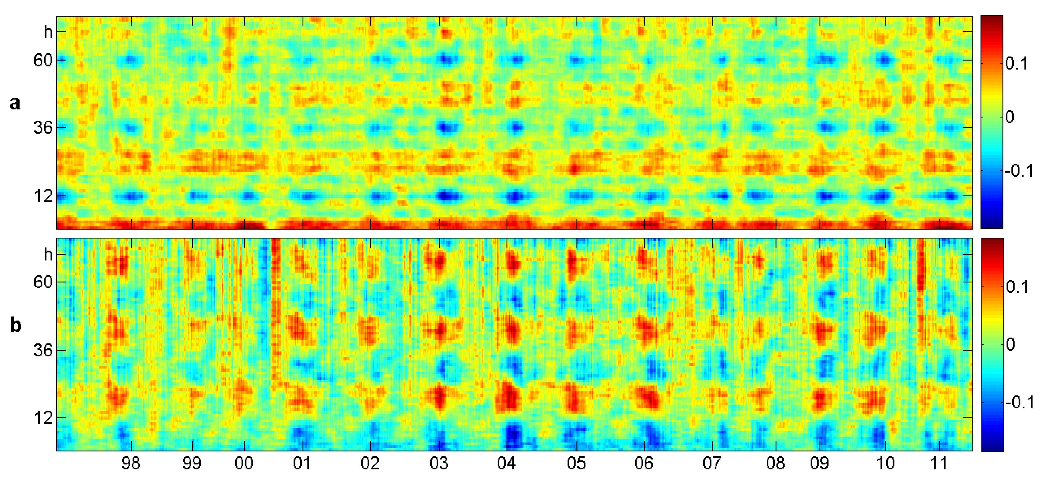
7. Case Study: Tides
7.1. The Data
7.2. Order Correlation
7.3. Relative Order Correlation
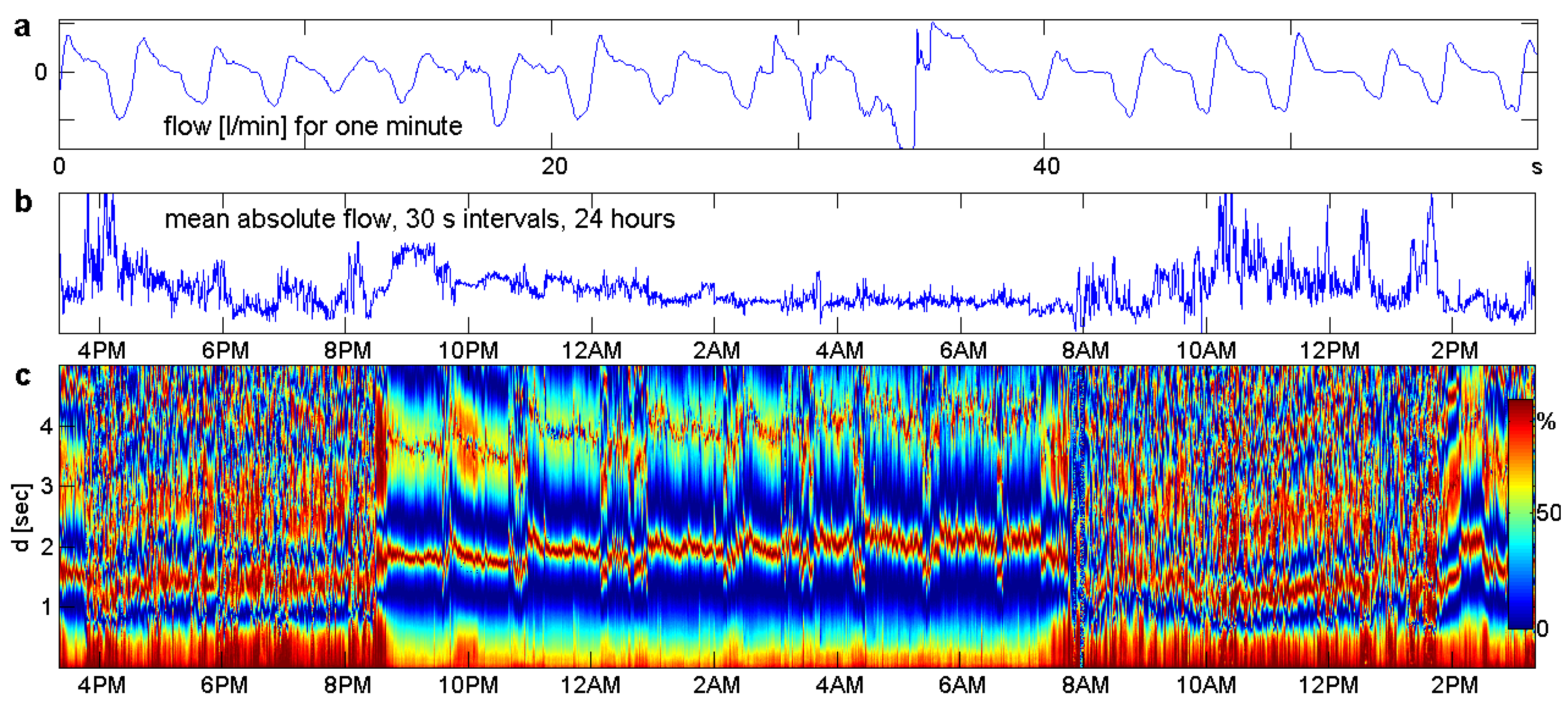
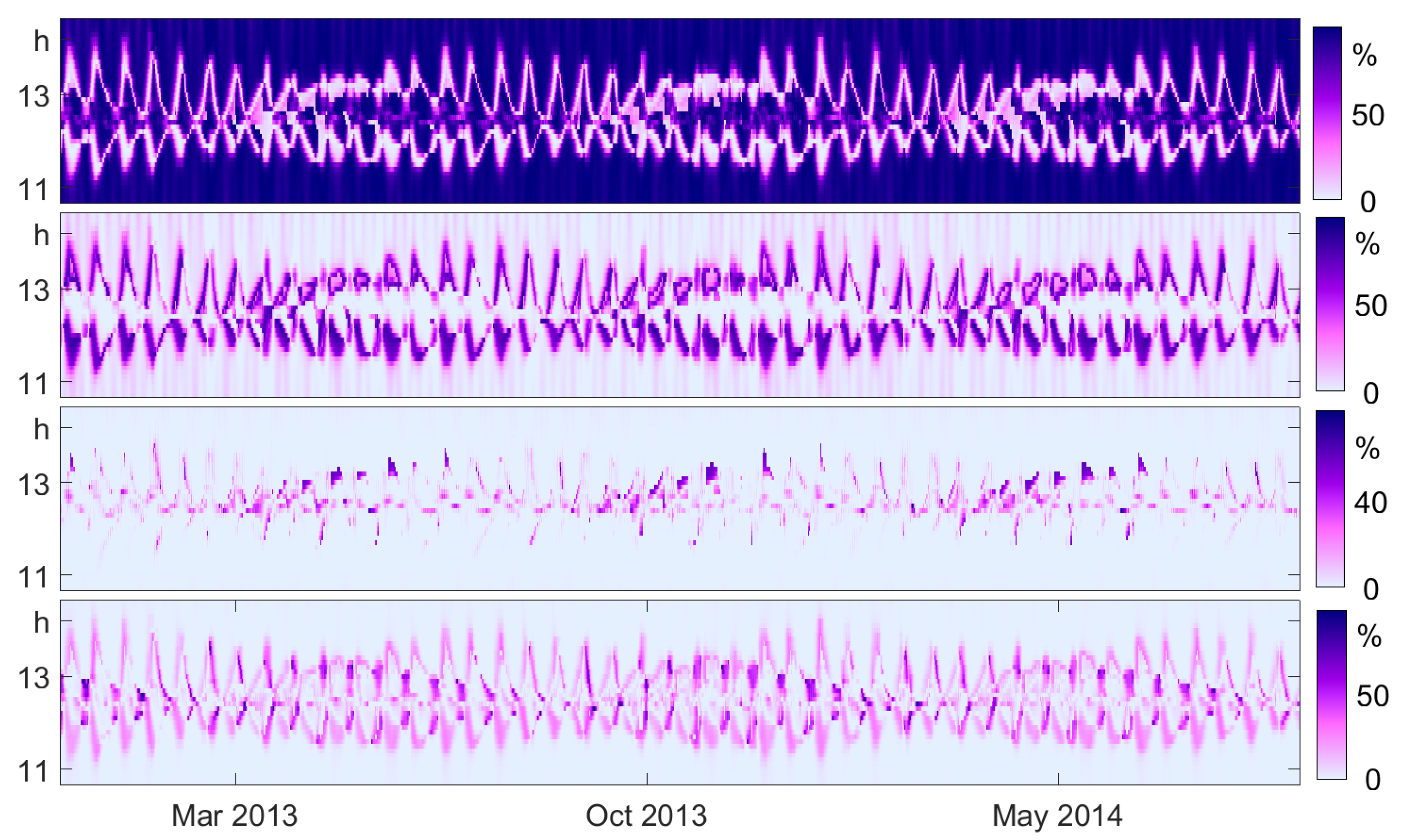
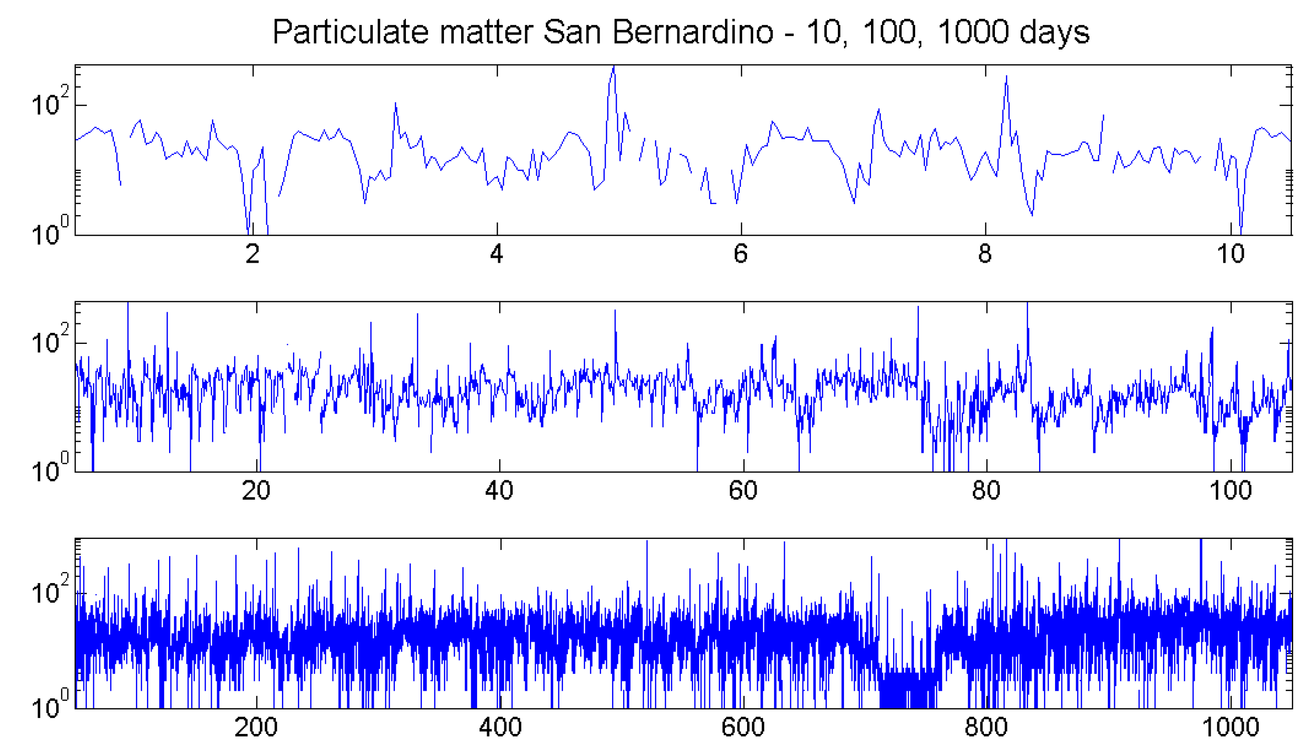
8. Case Study: Particulates
8.1. The Data
8.2. Sliding Windows Analysis
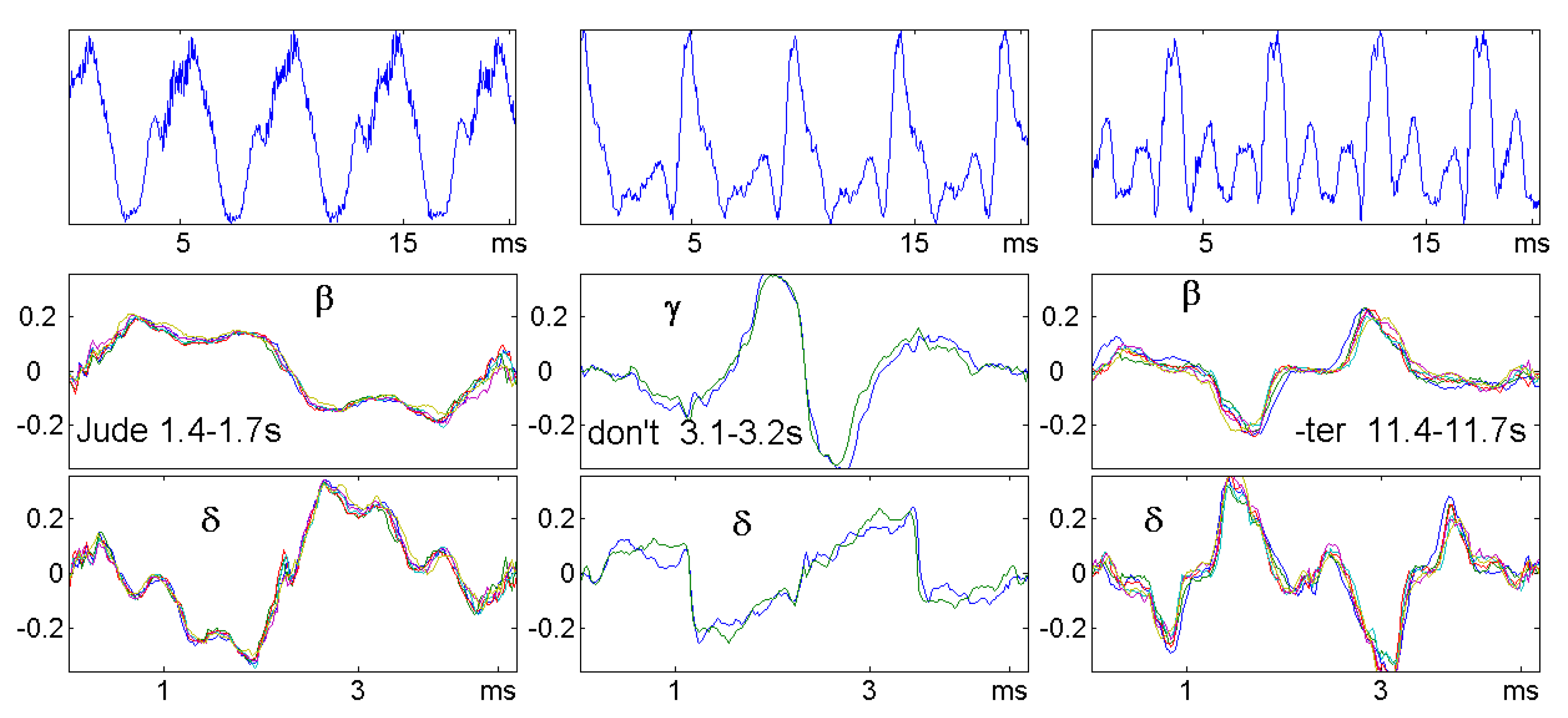
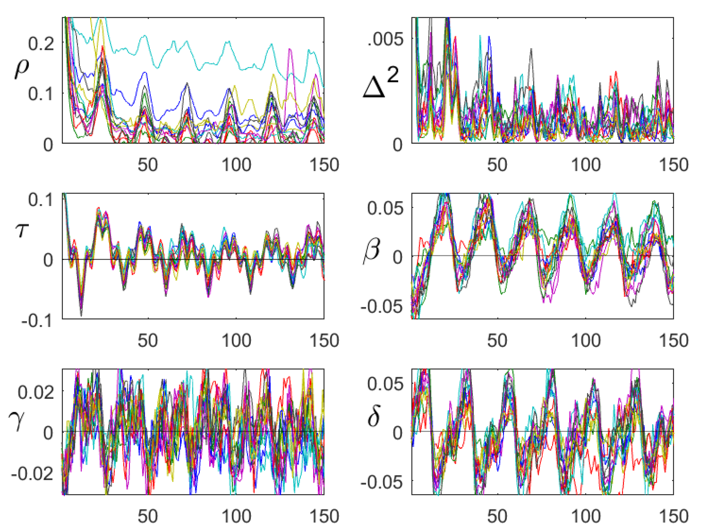
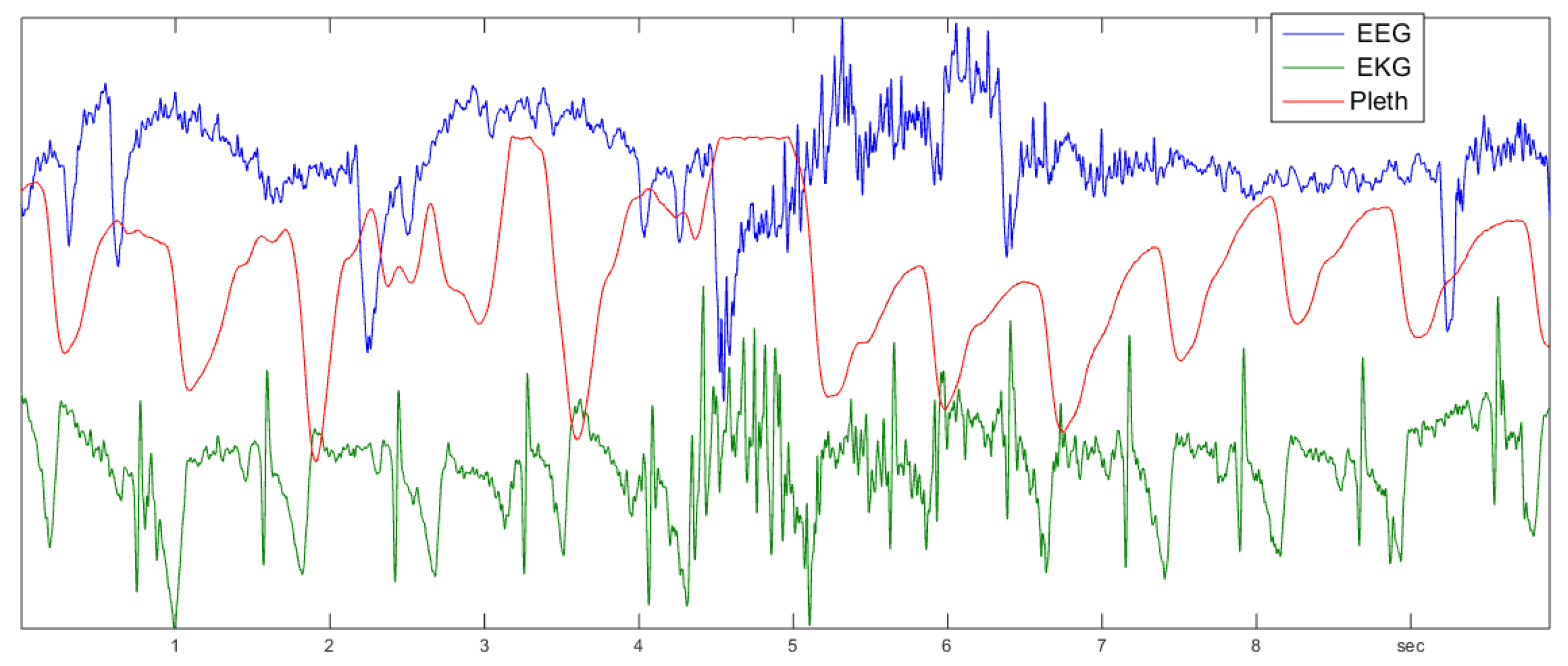
9. Brain and Heart Signals
9.1. The Data
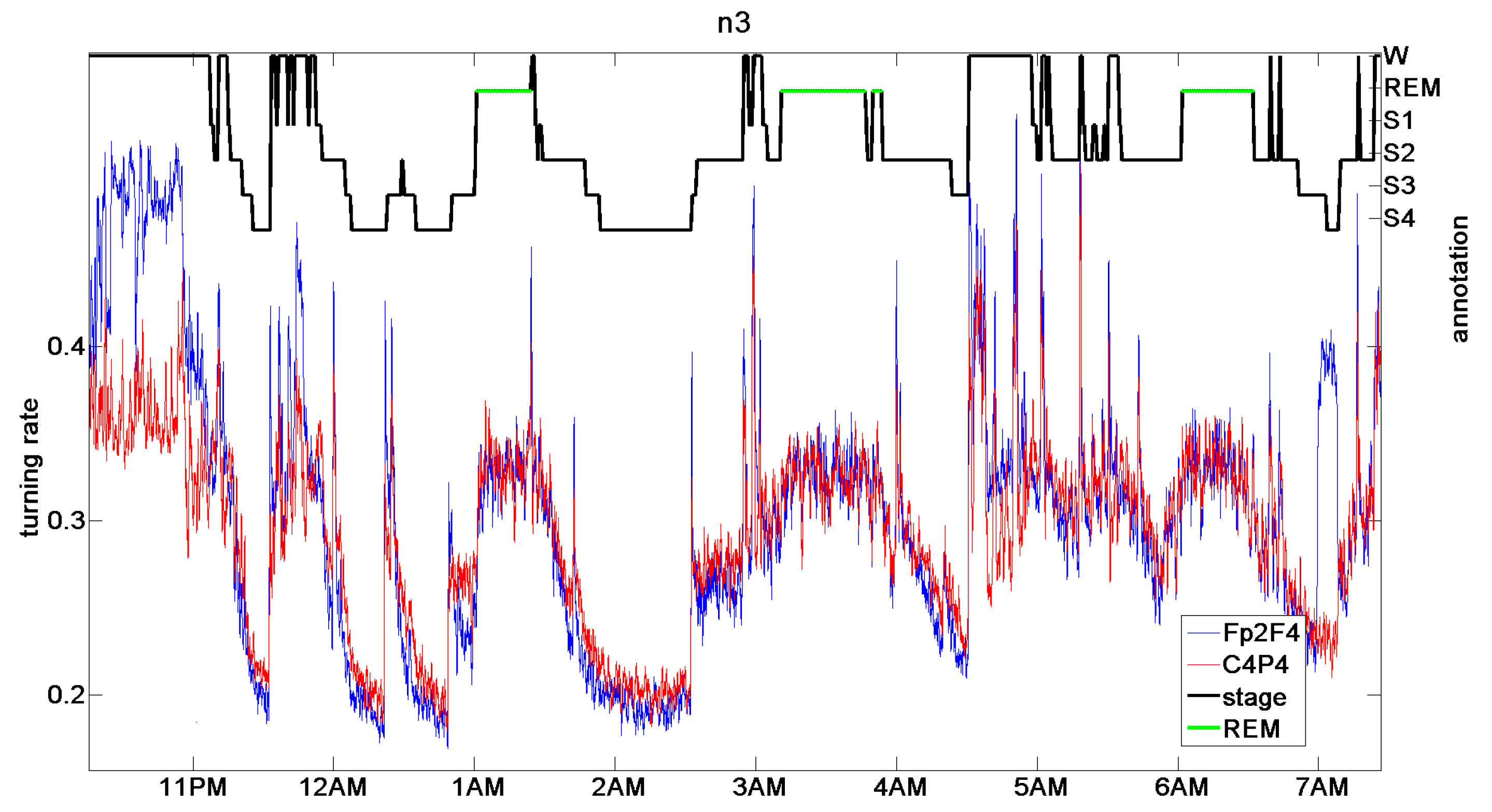
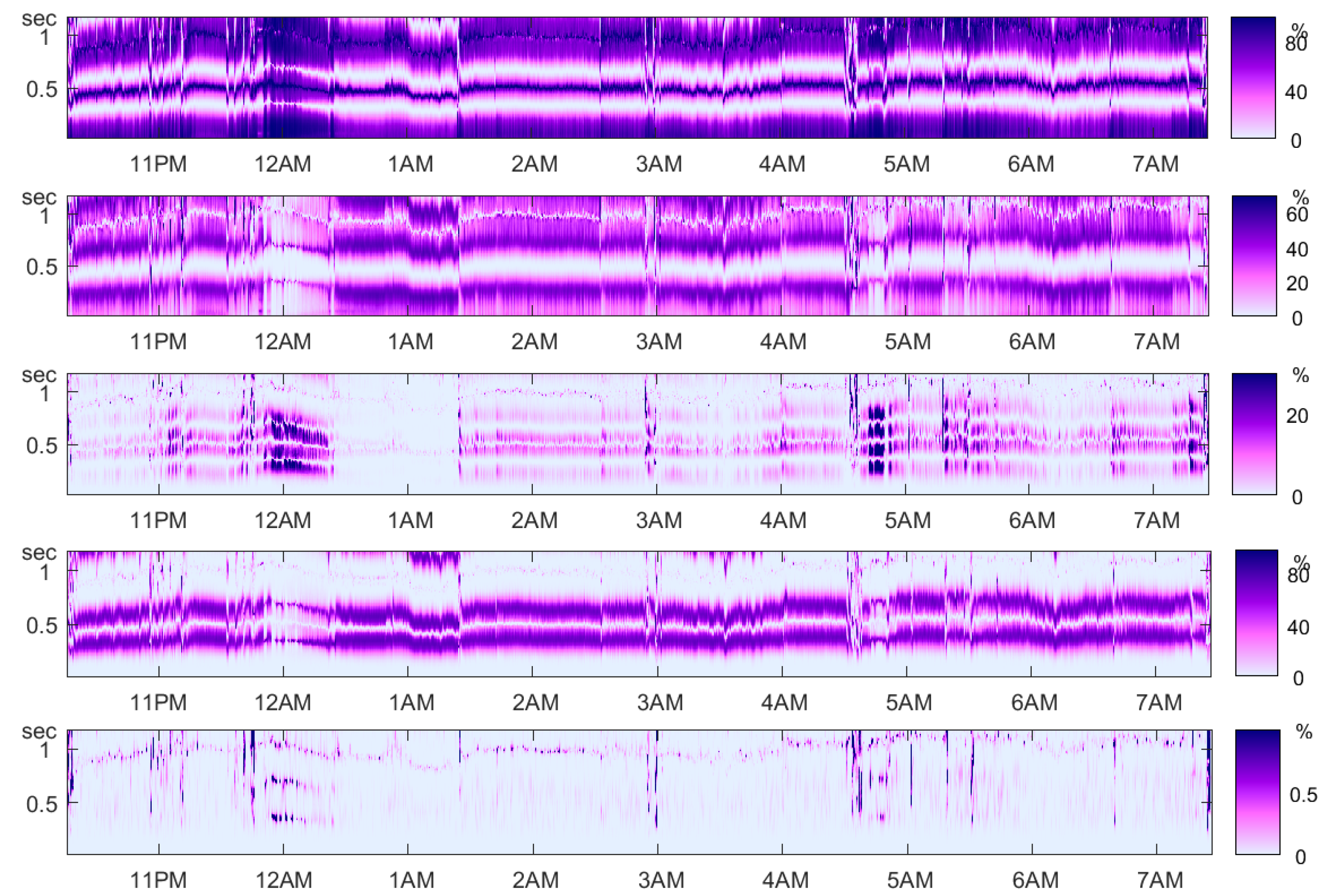
9.2. Sleep Stages
10. Conclusions
Funding
Acknowledgments
Conflicts of Interest
References
- Amigo, J.; Keller, K.; Kurths, J. Recent progress in symbolic dynamics and permutation complexity. Ten years of permutation entropy. Eur. Phys. J. Spec. Top. 2013, 222, 247–257. [Google Scholar]
- Amigo, J.M. Permutation Complexity in Dynamical Systems; Springer Series in Synergetics; Springer: Berlin, Germany, 2010. [Google Scholar]
- Zanin, M.; Zunino, L.; Rosso, O.; Papo, D. Permutation entropy and its main biomedical and econophysics applications: A review. Entropy 2012, 14, 1553–1577. [Google Scholar] [CrossRef]
- Carpi, L.C.; Saco, P.M.; Rosso, O.A. Missing ordinal patterns in correlated noises. Phys. A 2010, 389, 2020–2029. [Google Scholar] [CrossRef]
- Martinez, J.H.; Herrera-Diestra, J.L.; Chavez, M. Detection of time reversibility in time series by ordinal patterns analysis. Chaos 2018, 28, 123111. [Google Scholar] [CrossRef] [PubMed]
- Zanin, M.; Rodríguez-González, A.; Menasalvas Ruiz, E.; Papo, D. Assessing time series reversibility through permutation patterns. Entropy 2018, 20, 665. [Google Scholar]
- Parlitz, U.; Berg, S.; Luther, S.; Schirdewan, A.; Kurths, J.; Wessel, N. Classifying cardiac biosignals using ordinal pattern statistics and symbolic dynamics. Comput. Biol. Med. 2012, 42, 319–327. [Google Scholar] [CrossRef] [PubMed]
- McCullough, M.; Small, M.; Iu, H.; Stemler, T. Multiscale ordinal network analysis of human cardiac dynamics. Philos. Trans. R. Soc. A Math. Phys. Eng. Sci. 2017, 375, 20160292. [Google Scholar] [CrossRef]
- Bandt, C.; Shiha, F. Order patterns in time series. J. Time Ser. Anal. 2007, 28, 646–665. [Google Scholar] [CrossRef]
- Bandt, C. Permutation entropy and order patterns in long time series. In Time Series Analysis and Forecasting; Rojas, I., Pomares, H., Eds.; Contributions to Statistics; Springer: Berlin, Germany, 2015. [Google Scholar]
- Bandt, C. A new kind of permutation entropy used to classify sleep stages from invisible EEG microstructure. Entropy 2017, 19, 197. [Google Scholar] [CrossRef]
- Bandt, C.; Pompe, B. Permutation entropy: A natural complexity measure for time series. Phys. Rev. Lett. 2001, 88, 174102. [Google Scholar] [CrossRef] [PubMed]
- Bandt, C. Autocorrelation type functions for big and dirty data series. arXiv 2014, arXiv:1411.3904. [Google Scholar]
- Rosso, O.; Larrondo, H.; Martin, M.T.; Plastino, A.; Fuentes, M. Distinguishing Noise from Chaos. Phys. Rev. Lett. 2007, 99, 154102. [Google Scholar] [CrossRef] [PubMed]
- López-Ruiz, R.; Nagy, Á.; Romera, E.; Sañudo, J. A generalized statistical complexity measure: Applications to quantum systems. J. Math. Phys. 2009, 50, 123528. [Google Scholar] [CrossRef]
- Deutscher Wetterdienst. Climate Data Center. Available online: ftp://ftp-cdc.dwd.de/pub/CDC/observations_germany (accessed on 20 May 2019).
- Brockwell, P.; Davies, R. Time Series, Theory and Methods, 2nd ed.; Springer: New York, NY, USA, 1991. [Google Scholar]
- Shumway, R.; Stoffer, D. Time Series Analysis and Its Applications, 2nd ed.; Springer: New York, NY, USA, 2006. [Google Scholar]
- Bandt, C. Crude EEG parameter provides sleep medicine with well-defined continuous hypnograms. arXiv 2017, arXiv:1710.00559. [Google Scholar]
- Ferguson, S.; Genest, C.; Hallin, M. Kendall’s tau for serial dependence. Can. J. Stat. 2000, 28, 587–604. [Google Scholar] [CrossRef]
- National Oceanic and Atmospheric Administration. National Water Level Observation Network. Available online: https://www.tidesandcurrents.noaa.gov/nwlon.html (accessed on 20 May 2019).
- California Air Resources Board. Available online: www.arb.ca.gov/adam (accessed on 20 May 2019).
- Terzano, M.; Parrino, L.; Sherieri, A.; Chervin, R.; Chokroverty, S.; Guilleminault, C.; Hirshkowitz, M.; Mahowald, M.; Moldofsky, H.; Rosa, A.; et al. Atlas, rules, and recording techniques for the scoring of cyclic alternating pattern (CAP) in human sleep. Sleep Med. 2001, 2, 537–553. [Google Scholar] [CrossRef]
- Goldberger, A.; Amaral, L.; Glass, L.; Hausdorff, J.; Ivanov, P.; Mark, R.; Mietus, J.; Moody, G.; Peng, C.K.; Stanley, H. PhysioBank, PhysioToolkit, and PhysioNet: Components of a new research resource for complex physiologic signals. Circulation 2000, 101, e215–e220. [Google Scholar] [CrossRef] [PubMed]


| Function | Range | Min Assumed for | Max Assumed for |
|---|---|---|---|
| Autocorrelation | linear decreasing series | linear increasing series | |
| Spearman rank autocorr. | decreasing series | increasing series | |
| Up-down balance | decreasing series | increasing series | |
| Persistence | alternating series | monotone series | |
| Turning rate | monotone series | alternating series | |
| Up-down scaling | |||
| Rotational asymmetry |
| Function | Time Reversal | Negative Function | Rotation |
|---|---|---|---|
| Spearman, | + | − | − |
| and | − | − | + |
| Rotational asymmetry | − | + | − |
| Function | Half Period | Period L | Symmetry Type |
|---|---|---|---|
| Spearman, | minimum | maximum | vertical line |
| Persistence | minimum | bumped maximum | vertical line |
| and | zero | zero or discontinuity | symmetry center |
© 2019 by the author. Licensee MDPI, Basel, Switzerland. This article is an open access article distributed under the terms and conditions of the Creative Commons Attribution (CC BY) license (http://creativecommons.org/licenses/by/4.0/).
Share and Cite
Bandt, C. Small Order Patterns in Big Time Series: A Practical Guide. Entropy 2019, 21, 613. https://doi.org/10.3390/e21060613
Bandt C. Small Order Patterns in Big Time Series: A Practical Guide. Entropy. 2019; 21(6):613. https://doi.org/10.3390/e21060613
Chicago/Turabian StyleBandt, Christoph. 2019. "Small Order Patterns in Big Time Series: A Practical Guide" Entropy 21, no. 6: 613. https://doi.org/10.3390/e21060613
APA StyleBandt, C. (2019). Small Order Patterns in Big Time Series: A Practical Guide. Entropy, 21(6), 613. https://doi.org/10.3390/e21060613