Structural Characteristics of Two-Sender Index Coding

Abstract

This paper studies index coding with two senders. In this setup, source messages are distributed among the senders possibly with common messages. In addition, there are multiple receivers, with each receiver having some messages a priori, known as side-information, and requesting one unique message such that each message is requested by only one receiver. Index coding in this setup is called two-sender unicast index coding (TSUIC). The main goal is to find the shortest aggregate normalized codelength, which is expressed as the optimal broadcast rate. In this work, firstly, for a given TSUIC problem, we form three independent sub-problems each consisting of the only subset of the messages, based on whether the messages are available only in one of the senders or in both senders. Then, we express the optimal broadcast rate of the TSUIC problem as a function of the optimal broadcast rates of those independent sub-problems. In this way, we discover the structural characteristics of TSUIC. For the proofs of our results, we utilize confusion graphs and coding techniques used in single-sender index coding. To adapt the confusion graph technique in TSUIC, we introduce a new graph-coloring approach that is different from the normal graph coloring, which we call two-sender graph coloring, and propose a way of grouping the vertices to analyze the number of colors used. We further determine a class of TSUIC instances where a certain type of side-information can be removed without affecting their optimal broadcast rates. Finally, we generalize the results of a class of TSUIC problems to multiple senders.

1. Introduction

Consider a communication scenario over a noiseless channel where a sender is required to broadcast messages to multiple receivers, each caching some messages requested by other receivers a priori. The messages cached at each receiver is known as its side-information. In this scenario, if the sender is informed about the side-information available at all receivers, then it can leverage that information whilst encoding to reduce the required number of broadcast transmissions, in comparison with a naive approach of transmitting all requested messages uncoded and separately. Such an encoding process is called index coding, and the resulting sequence of coded messages is known as an index code. Moreover, each receiver upon receiving the index code will be able to decode its required message by utilizing its side-information. The main aim of index coding is to find the optimal (shortest) codelength and the corresponding coding scheme. Index coding was introduced by Birk and Kol [1,2], and further studied in subsequent works [3,4,5,6,7,8,9,10,11,12,13].

Most existing works on index coding deal only with a single sender, capturing scenarios with centralized transmissions. However, many communication scenarios such as the following have messages distributed among multiple senders:

• Macro-cell networks with caching helpers [14]—cellular networks deploying dedicated nodes, called helpers, with large storage capacity instead of femto-cell access points to reduce backhaul loads,
• cooperative data exchange [15]—peer-to-peer networks with data exchange within a group of closely-located wireless nodes, and
• distributed storage—storage networks where data are distributed over multiple storage devices/locations.

In addition, each sender can be constrained to know only a subset of the total messages due to reasons such as limited storage, or error whilst receiving some messages over noisy channels, or server failure to deliver all messages. In this case, distributed transmissions are required, where multiple senders broadcast messages to the receivers. One metric to maximize the transmission efficiency in this scenario is to minimize the aggregate number of transmissions from all senders in such a way that all receivers’ demands can be fulfilled. As this problem is more general than an index-coding problem with a single sender and is of practical interest (e.g., reducing delay in content delivery, and energy efficient broadcasting), it is a useful research avenue to study index-coding problems with multiple senders, known as multi-sender index-coding problems.

1.1. Prior Works

The multi-sender index-coding problem was first studied by Ong et al. [16]. They considered the problems where multiple senders are connected to receivers via noiseless broadcast links (orthogonal to each other) with flexible capacities. In their setup, each sender knows only a subset of the messages; each receiver knows only one message requested by some receiver a priori, but may request multiple messages; in addition, one message is known to only one receiver. For this setup, they aimed to characterize the optimal aggregate codelengths, also known as the optimal broadcast rates, of the problems. This problem formulation model is called broadcast-rate formulation of the problems. In their work, they devised lower and upper bounds on the optimal broadcast rate by implementing a graph-theoretic approach. The results were established using information-flow graphs, which represent receivers’ request, and message graphs, which represent senders’ message setting. Furthermore, they showed problem instances for which the upper and lower bounds coincide. A class of such instances is where no two senders have messages in common.

In another work, Thapa et al. [17] considered a model similar to Ong et al. [16] but with the unicast message setting, meaning each message is requested by only one receiver, each receiver requests only one message, and each receiver knows a subset of messages requested by other receivers a priori. Based on graph-theoretic approaches, they established upper bounds on the optimal broadcast rate. In particular, they focused on the two-sender case, called two-sender unicast index coding (TSUIC). They extended existing single-sender index-coding schemes, namely the cycle-cover scheme [18,19], the clique-cover scheme [1,2] and the local-chromatic scheme [10] to the corresponding schemes in TSUIC.

Sadeghi et al. [20] considered multi-sender index-coding problems where the senders are connected to receivers via noiseless broadcast links of arbitrary but fixed capacities. They aimed to characterize the closure of the set of all achievable rate tuples of messages, known as the capacity region. The rate of a message is the number of message bits per encoded/broadcast bits. They devised inner bounds on the capacity region using random-coding approaches (which requires infinitely long messages), and outer bounds using Shannon-type inequalities. In particular, the first general inner bound was attained by a partitioned distributed-composite-coding scheme, built on the single-sender composite-coding scheme (an existing single-sender scheme that is based on a random-coding approach [7]). This scheme was further enhanced to a fractional distributed-composite-coding scheme by Liu et al. [21]. Preliminary and improved polymatroidal outer bounds were also developed in the work by Sadeghi et al. [20] and Liu et al. [21], respectively. As a result, the capacity region was established for all problem instances up to three receivers, and the sum capacity is established for all instances with four receivers and with unit link capacity from each sender. Independent of and in parallel with the work by Liu et al. [21], Li et al. [22,23] introduced new techniques of joint link-and-sender partitioning and cooperative compression of composite messages and developed a multi-sender cooperative composite-coding scheme.

In a recent work by Li et al. [24], a new rank-minimization framework for multiple-sender index coding with the unicast message setting, i.e., MSUIC, was developed on the classic single-sender minrank concept. The framework enabled the authors to establish the optimal broadcast rate for all critical MSUIC instances up to four receivers. In addition, they presented a heuristic algorithm to study MSUIC instances with more receivers. Wan et al. [25] introduced decentralized data shuffling problems in which the receivers/workers can communicate with one another via a shared link. The decentralized data shuffling phase with uncoded storage (which stores a subset of bits of the data set) is equivalent to a multi-sender index coding problem. For this problem, they proposed converse and achievable bounds that are to within a factor of 3/2 of one another. Moreover, the proposed schemes were shown to be optimal for some classes of the problem. Recently, Porter et al. [26] introduced a special case of multi-sender index coding, called embedded index coding (EIC), in which each node acts as both sender and receiver. With the help of several results, they showed the relationship between single-sender index coding and EICs. Furthermore, they developed heuristics to solve EIC problems efficiently.

1.2. Our Work and Contributions

Different approaches have been attempted to solve the multi-sender index-coding problems. However, the problems are more difficult and computationally complex than their single-sender counterparts, and we know very little about the characteristics of the problems. This paper studies the broadcast-rate formulation of TSUIC problems by implementing a graph-theoretic approach. More precisely, in the same spirit of studying structural properties of index-coding capacity in the single-sender case by Arbabjolfaei et al. [8], we examine the structural characteristics of TSUIC problems. This kind of study embraces the “divide-and-conquer” approach and provides us an insight into the problems where we can solve a larger problem by solving its smaller sub-problems. Note that, in the work by Arbabjolfaei et al. [8,27], the capacity region of a given single-sender index-coding problem is shown to be a simple function of the capacity regions of its independent sub-problems by generalizing the notion of lexicographic graph product. In the TSUIC setup, due to the distributed message setting among senders, we cannot directly implement the notion of graph products and the existing approaches of single-sender index coding. In this work, we consider interactions between three independent sub-problems at a time in the TSUIC setup. By applying the notion of confusion graphs in index coding [28] along with the introduction of a two-sender graph coloring and a code-forming technique, we bound the optimal broadcast rate in both asymptotic and non-asymptotic regimes, and show it to be tight for some classes of TSUIC instances. Moreover, even for the single-sender cases, the non-asymptotic cases (especially index coding in nonlinear, finite fields) are less explored. For an index coding instance in the unicast message setting and the non-asymptotic regime in the message size, our techniques in this paper can be used to upper bound the optimal broadcast rate of this instance by a function of the optimal broadcast rates of its sub-instances in single-sender unicast index coding.

The contributions of this paper are summarized as follows:

• Proposing a new coloring concept for confusion graphs in TSUIC, called two-sender graph coloring (Definition 8, Section 4.3): For SSUIC, the chromatic number of its confusion graph gives the optimal broadcast rate and the corresponding index code (for a specific message size). However, for TSUIC, as the two senders (encoders) contain some messages in common, the standard method of graph coloring of the confusion graph may not lead us to an index code. In this regard, we need a different kind of coloring function in TSUIC, and thus, in this paper, we propose a novel coloring technique to color the confusion graphs in TSUIC, and its optimization gives the optimal broadcast rate and optimal index code.
• Presenting a way of grouping the vertices of confusion graphs in TSUIC (Appendix B): By exploiting the symmetry of the confusion graph, we propose a way of grouping its vertices for analysis purposes mainly in its two-sender graph coloring. In particular, this grouping helps us to analyze the number of colors used in two-sender graph coloring of a confusion graph.
• Deriving the optimal broadcast rates of TSUIC problems as a function of the optimal broadcast rates of its sub-problems (Theorems 4–8): We divide a TSUIC problem into three independent sub-problems based on the requested messages by receivers, specifically whether the messages are present in only one of the senders or in both senders. Now in TSUIC, considering the interactions (defined by side-information available at the receivers) between these three independent sub-problems, we derive the optimal broadcast rate (in both asymptotic and non-asymptotic regimes in the message size) of the problem as a function of the optimal broadcast rates of its sub-problems. Moreover, we bound the optimal broadcast rate, and show that the bounds are tight for several classes of TSUIC instances (sometimes with conditions). Furthermore, we find a class of TSUIC instances where a TSUIC scheme can achieve the same optimal broadcast rate as the same instances when the two senders form a single sender having all messages.
• Characterizing a class of TSUIC instances where a certain type of side-information is not critical (Corollary 1): For a class of TSUIC instances, we prove that certain interactions between the three independent sub-problems can be removed without affecting the optimal broadcast rate (in the asymptotic regime). This means that those interactions are not critical.
• Generalizing the results of some classes of TSUIC problems to multiple senders (Section 6): For some classes of TSUIC problems, we generalize the two-sender graph coloring of confusion graphs and the proposed grouping of their vertices. Then, we compute the optimal broadcast rates of those problems as a function of the optimal broadcast rates of their sub-problems.

After posting the first draft of this paper [29] on Arxiv, this work had led to the following works in TSUIC. Arunachala et al. [30,31] claimed that they derived the optimal linear broadcast rates of classes of TSUIC problems as a function of their sub-problems by analyzing special matrices and linear code constructions. In another work by Arunachala et al. [32], the optimal asymptotic broadcast rates (asymptotic in the message size) of TSUIC problems were derived as a function of their sub-problems with fully-participated interactions. They affirmed that, for some classes of TSUIC problems, the upper bounds of the optimal broadcast rates presented in our paper are tight. For their results, they used a similar graph-based technique as presented in our first draft ([29]). In this paper, we consider general broadcast rates (which includes both linear and nonlinear, broadcast rates) for both asymptotic and non-asymptotic regimes in the message size.

2. Problem Definitions and Graphical Representation

2.1. Problem Setup

In this paper, we consider unicast index coding. There are N independent messages $\mathcal{M}=\{x_1,x_2,\cdots ,x_N\}$, where $x_i\in {\{0,1\}}^t$ for all $i\in \{1,2\cdots ,N\}$ and some integer $t\ge 1$, i.e., each message consists of t binary bits. There are N receivers $\{1,2,\cdots ,N\}$, where each receiver $r\in \{1,2,\cdots ,N\}$ requests a message $x_r$, and has an ordered set ${\mathcal{H}}_r\subseteq \mathcal{M}\backslash \left\{x_r\right\}$ of messages as its side-information a priori. In the ordered set, the elements are arranged in increasing indices. This paper deals with the following two types of unicast index coding (UIC) based on the number of senders: (i) Single-sender unicast index coding (SSUIC)—it has only one sender, denoted S, having all N messages $\mathcal{M}$, and (ii) two-sender unicast index coding (TSUIC)—it has two senders, denoted by $S_1$ and $S_2$, having (ordered) message sets ${\mathcal{M}}_1\subseteq \mathcal{M}$ and ${\mathcal{M}}_2\subseteq \mathcal{M}$, respectively, such that ${\mathcal{M}}_1\cup {\mathcal{M}}_2=\mathcal{M}$ (i.e., each message is available at some sender(s)). In other words, the total messages are distributed over the two senders in TSUIC. Figure 1 illustrates an example of TSUIC problems with four receivers. Given an index-coding problem, a two-sender index code is defined as follows:

Definition 1 (Two-sender index code).

A two-sender index code ($\left\{{\mathcal{F}}_s\right\},\left\{{\mathcal{G}}_r\right\}$), for $s\in \{1,2\}$, $r\in \{1,2,\cdots ,N\}$, is defined by

(i) 

an encoding function for each sender $S_s$, ${\mathcal{F}}_s:{\{0,1\}}^{|{\mathcal{M}}_s|\times t}\to {\{0,1\}}^{p_s}$ such that ${\mathcal{C}}_s={\mathcal{F}}_s({\mathcal{M}}_s)$, and

(ii) 

a decoding function for every receiver r, ${\mathcal{G}}_r:{\{0,1\}}^{({\Sigma }_{s=1}^2{p}_s+|{\mathcal{H}}_r|\times t)}\to {\{0,1\}}^t$ such that $x_r={\mathcal{G}}_r({\mathcal{C}}_1,{\mathcal{C}}_2,{\mathcal{H}}_r)$.

This means that each sender $S_s$ encodes its known messages to a $p_s$-bit sub-codeword, for some non-negative integer $p_s$. We assume that each receiver r receives sub-codewords from both senders without any noise, and decodes $x_r$ from the received sub-codewords and ${\mathcal{H}}_r$. The sub-codewords $({\mathcal{C}}_1,{\mathcal{C}}_2)$ form an index code in TSUIC.

Now, we define the aggregate normalized codelength, which measures the performance of a code $({\mathcal{C}}_1,{\mathcal{C}}_2)$, in the following.

Definition 2 (Broadcast rate or aggregate normalized codelength).

The broadcast rate of an index code (with a single sender or two senders) is the total number of transmitted bits (if two senders, then it is a sum of transmitted bits by both senders) per received message bit. In TSUIC, it is denoted by ${\ell }_{\mathsf{TSUIC}}\triangleq \frac{(p_1+p_2)}{t}$ for an index code ($\left\{{\mathcal{F}}_s\right\},\left\{{\mathcal{G}}_r\right\}$). The broadcast rate is also referred to as the aggregate normalized codelength of the index code. We say that ℓ is achievable for a UIC problem if there exists an index code of normalized length ℓ.

For the rest of the paper, we refer to normalized codelength simply as codelength.

Definition 3 (Optimal broadcast rate).

The optimal broadcast rate for a given index-coding problem with t-bit messages is ${\beta }_t\triangleq \underset{\mathcal{E}}{\min }\ell$, where $\mathcal{E}=\mathcal{F}$ for SSUIC and $\mathcal{E}=\left\{{\mathcal{F}}_s\right\}$ for TSUIC. The optimal broadcast rate over all t is defined as $\beta \triangleq \underset{t}{\inf }{\beta }_t=\underset{t\to \infty }{\lim }{\beta }_t$. The limit exists and is equal to the infimum due to the subadditivity of $t{\beta }_t=p_1+p_2$ and Fekete’s lemma [33].

Remark 1.

With the (optimal) broadcast rate as a performance metric, we can treat SSUIC as a special case of TSUIC when ${\mathcal{M}}_1=\mathcal{M}$ or ${\mathcal{M}}_2=\mathcal{M}$. Furthermore, for this case, the sender with $\mathcal{M}$ alone will be responsible for fulfilling the demands made by all receivers.

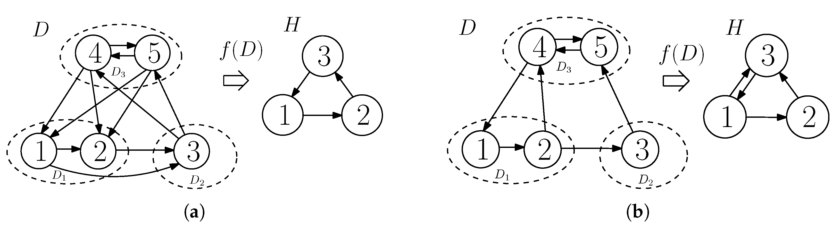
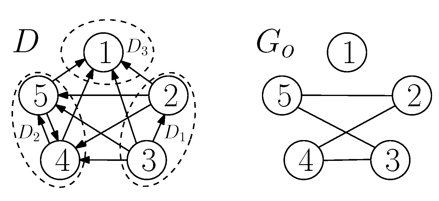
2.2. Representation of the Receivers’ Side-Information and the Senders’ Message Setting in TSUIC Problems

An index-coding problem can be modeled by graphs, which are defined as follows:

Definition 4 (Directed graphs and undirected graphs).

A directed graph is an ordered pair $D=(V(D),A(D))$, where $V(D)$ is a set of vertices, and $A(D)$, usually called an arc set, is a set of ordered pairs of vertices. An undirected graph is an ordered pair $G=(V(G),E(G))$, where $V(G)$ is a set of vertices, and $E(G)$, usually called an edge set, is a set of unordered pairs of vertices.

From now on in this paper, we call directed graphs simply digraphs, and undirected graphs simply graphs.

The receivers’ message setting of a UIC problem is represented by a side-information digraph $D=(V(D),A(D))$, where $V(D)=\{1,2,\cdots ,N\}$ represents the N receivers, and the arc set $A(D)$ represents the side-information available at each receiver. More precisely, an arc $(i,j)\in A(D)$ exists from vertex i to vertex j if and only if receiver i has message $x_j$ (the message requested by receiver j) in its side-information. Thus, in a side-information digraph, ${\mathcal{H}}_i\triangleq \{x_j:j\in N_D^{+}(i)\}$, where $N_D^{+}(i)$ is the out-neighborhood of a vertex i in D. In this paper, for convenience, a receiver i is also referred to as a vertex i, and vice versa. We also use the compact form of representation of an instance of UIC problems as used by Arbabjolfaei et al. [7], where a sequence $(i|N_D^{+}(i))$, for all $i\in V(D)$, represents a UIC problem.

In TSUIC, $S_1$ (sender one) encodes the messages in ${\mathcal{M}}_1$, and $S_2$ (sender two) encodes the messages in ${\mathcal{M}}_2$. In general, each sender has private messages and common messages defined as follows: Let ${\mathcal{P}}_1\triangleq {\mathcal{M}}_1\backslash {\mathcal{M}}_2$ and ${\mathcal{P}}_2\triangleq {\mathcal{M}}_2\backslash {\mathcal{M}}_1$ be the set of private messages at senders $S_1$ and $S_2$, respectively, and ${\mathcal{P}}_3\triangleq {\mathcal{M}}_1\cap {\mathcal{M}}_2$ be the set of common messages at both senders. Now, for a given side-information digraph D, without loss of generality, we define the following sub-digraphs induced by the following vertex subsets that partition $V(D)$: For $i\in \{1,2,3\}$, let $D_i$ be the sub-digraph of D induced by vertices $\{j:x_j\in {\mathcal{P}}_i\}$. We refer to $D_1$, $D_2$ and $D_3$ as per this definition throughout this paper unless stated otherwise. From the definition, it is clear that $D_1$, $D_2$ and $D_3$ are the three sub-digraphs of D such that $V(D)=V(D_1)\cup V(D_2)\cup V(D_3)$ and $V(D_i)\cap V(D_k)=\varnothing$ for any $i\ne k$, $i,k\in \{1,2,3\}$. In TSUIC, the senders are limited to transmit only their messages, and this limitation is defined formally as a constraint due to the two senders as follows:

Definition 5 (Constraint due to the two senders).

The constraint due to the two senders is the following: whilst encoding, any two private messages $x_i\in {\mathcal{P}}_1$ and $x_j\in {\mathcal{P}}_2$ should not be encoded together (with or without other messages) to construct one coded symbol, or alternatively any two-sender index code can be written as $({\mathcal{C}}_1,{\mathcal{C}}_2)$ such that ${\mathcal{C}}_1={\mathcal{F}}_1(\mathcal{M}\backslash {\mathcal{P}}_2)$ and ${\mathcal{C}}_2={\mathcal{F}}_2(\mathcal{M}\backslash {\mathcal{P}}_1)$.

In TSUIC, to reflect the senders’ message setting, we introduce an undirected graph, denoted by $G_o=(V(G_o),E(G_o))$ that is constructed in the following way: (i) $V(G_o)=V(D)$, and (ii) for all $i,j\in V(G_o)$, an undirected arc, i.e., an edge $(i,j)\in E(G_o)$ exists if and only if $x_i\in {\mathcal{P}}_1$ and $x_j\in {\mathcal{P}}_2$, or vice versa. This means, there is an edge connecting two vertices in $G_o$ if and only if no sender has both the corresponding messages. We call the graph $G_o$ the sender-constraint graph.

As a TSUIC problem is described by D and $G_o$, it is represented by $(D,G_o)$ in this paper. For a given $(D,G_o)$, let $\ell (D,G_o)$ denote the index codelength, ${\beta }_t(D,G_o)$ and $\beta (D,G_o)$ represent the optimal broadcast rate for a fixed t, and over all t, respectively. $\ell (D)$, ${\beta }_t(D)$ and $\beta (D)$ are the respective terms used for single-sender problems.

3. A New Way of Classifying TSUIC Problems and Main Results

In a TSUIC problem, if there is no common message, i.e., ${\mathcal{P}}_3=\varnothing$, then in our earlier work, we have proved that the problem is equivalent to two separate SSUIC problems ([17], Theorem 1). However, if ${\mathcal{P}}_3\ne \varnothing$, then the problem is less well understood. We propose to tackle this problem by dividing it into three sub-problems based on the type of messages at the senders (whether they are common or private), and then study the interactions among these sub-problems due to the side-information present at the receivers. In this way, we can devise the structural characteristics of TSUIC problems. For a given problem D, three sub-problems based on the type of messages are $D_1$, $D_2$ and $D_3$. The side-information present at receivers of one sub-problem about messages requested by receivers of other sub-problems are formally referred to as an interaction between those sub-problems, defined in the following. We will see that this allows us to derive ${\beta }_t(D,G_o)$ in terms of the single-sender characterizations $\{{\beta }_t(D_i):i\in \{1,2,3\}\}$ for a number of TSUIC instances.

3.1. Interactions between $D_1$, $D_2$ and $D_3$

Arcs between $V(D_1)$, $V(D_2)$ and $V(D_3)$, each originating from some vertices of $V(D_i)$, $i\in \{1,2,3\}$, and terminating at some vertices of $V(D)\backslash V(D_i)$ in D are called an interaction between $D_1$, $D_2$ and $D_3$. It is called a fully-participated interaction between $D_1$, $D_2$ and $D_3$ if and only if we have the following: If there exists an arc from a vertex of $D_i$ to a vertex of $D_j$ for any $i,j\in \{1,2,3\},i\ne j$, then $V(D_j)\subseteq N_D^{+}(r)$ for every $r\in V(D_i)$. In other words, all the vertices of the sub-digraph $D_i$ interact in the same way to all the vertices of the sub-digraph $D_j$. For an example of a fully-participated interaction, see Figure 2a. If an interaction between the sub-digraphs is not a fully-participated interaction, then it is called a partially-participated interaction among the sub-digraphs of the digraph. For example of a partially-participated interaction, see Figure 2b. For the sub-digraphs of D, if some vertices in $V(D_i)$ have out-going arcs to some vertices in $V(D_j)$, $i\ne j,i,j\in \{1,2,3\}$, then it is denoted as $D_i\to D_j$. If we write $D_i\rightleftarrows D_j$, then it means $D_i\to D_j$ and $D_j\to D_i$. These representations are used for the indication of interaction, which does not explicitly specify the type of interactions.

3.2. A Compact Representation of Interactions

For simplicity, an interaction between the sub-digraphs $D_1$, $D_2$ and $D_3$ of D can be viewed as an interaction between three vertices, where each vertex represents one of the sub-digraphs. In this regard, we define a function that maps a digraph D (with its sub-digraphs $D_1$, $D_2$ and $D_3$) to a digraph having three vertices, denoted H, in the following: $f:D\to H$ such that (i) all the vertices in $V(D_i)$ are mapped to a single vertex i of H, so $V(H)=\{1,2,3\}$, and (ii) $(i,j)\in A(H)$ if and only if there exist an arc $(u,v)\in A(D)$ for some $u\in V(D_i)$ and some $v\in V(D_j)$. For example, see Figure 2. By referring to the definition of the fully or partially participated interaction, one can find that, for a given $D_1$, $D_2$ and $D_3$ of D, we can retrieve D by observing $f(D)$ if D has a fully-participated interaction among the sub-digraphs, but this is not true if D has a partially-participated interaction among the sub-digraphs. Observe that, for any D, $D_i\to D_j$, if and only if $i\to j$ in $f(D)$ (i.e., H).

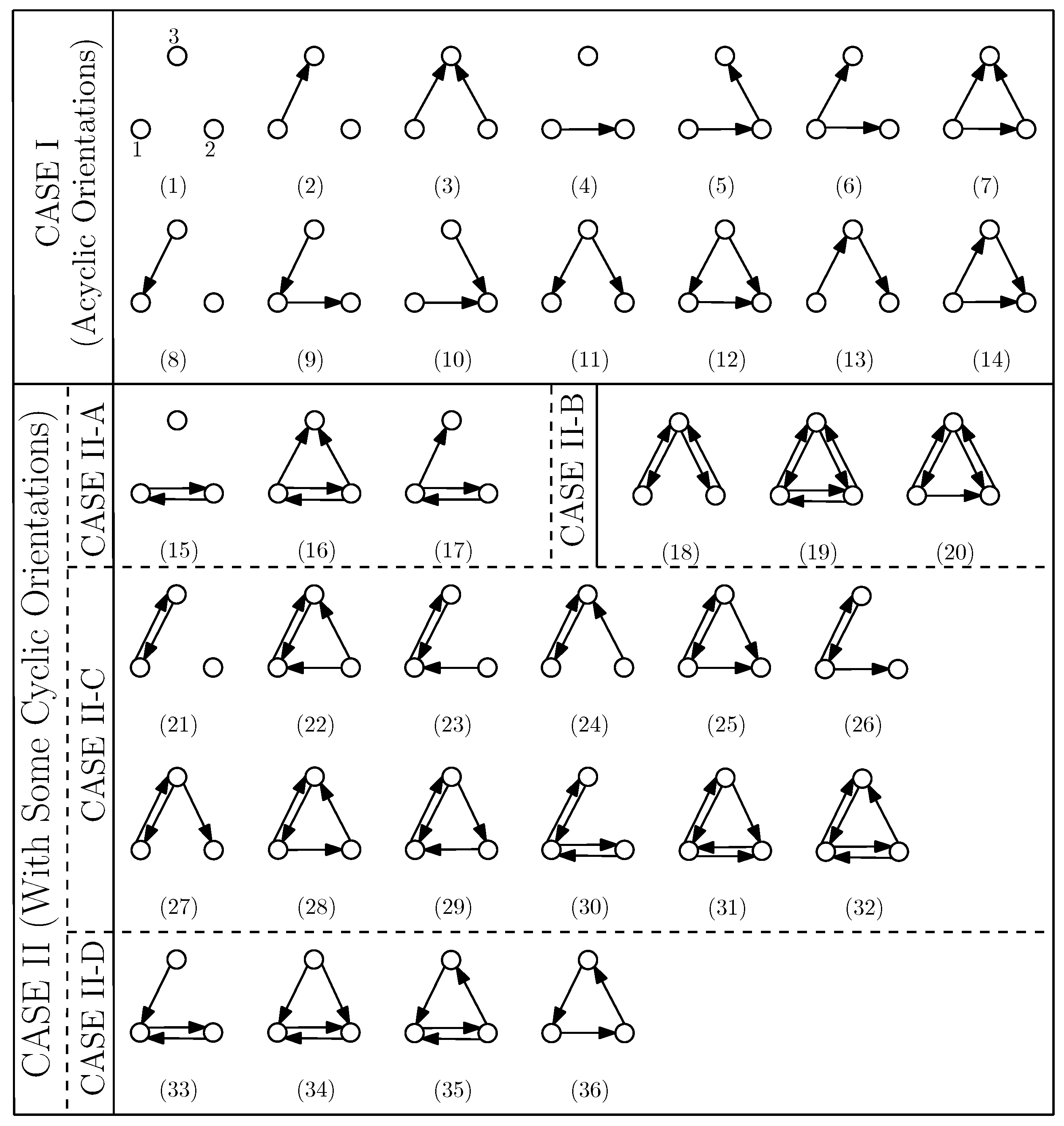
3.3. A Classification of the Interactions

Considering the digraph H, we get a total of 64 possible cases of the orientation of arcs among its vertices. As the vertices 1 and 2 of H can be swapped because we can interchange $D_1$ and $D_2$ (by swapping the labels of the senders), we get 36 unique cases (out of 64 cases) of interactions between the vertices of H. Now, depending upon the type of orientation of arcs among the vertices of H, we classify all unique cases into two categories: (i) CASE I—Acyclic orientation (14 cases in total), and (ii) CASE II—with some cyclic orientation (22 cases). CASE II is further classified into smaller sub-cases II-A, II-B, II-C, and II-D. Refer to Figure 3 for details, where each digraph of H is labeled ${\mathrm{H}}_i$ for $i\in \{1,2,\cdots ,36\}$. Note that an interaction between $D_1$, $D_2$ and $D_3$ of D defines arcs between them (not within the sub-digraph), and the cases of interactions (acyclic or cyclic) are defined with respect to the orientation of the arcs between the sub-digraphs. In this paper, a fully-participated interaction and a partially-participated interaction between $D_1$, $D_2$ and $D_3$ of D are called a cyclic-fully-participated interaction and a cyclic-partially-participated interaction between the sub-digraphs, respectively, if and only if $f(D)$ has some cycles (for example, see CASE II in Figure 3).

3.4. Main Results

For SSUIC, Arbabjolfaei and Kim [8] (Prop. 1) argued that using structural properties can reduce the number of problems that need to be studied. This paper investigates the structural characteristics of TSUIC problems for the same purpose by studying the interactions among $D_1$, $D_2$ and $D_3$ of D. Moreover, structural properties can be used to determine the criticality/non-criticality of arcs in TSUIC as in its SSUIC counterpart [9,34]. An arc is said to be critical if removing the arc strictly increases the optimal broadcast rate.

This paper analyzes all cases of fully-participated and some cases of partially-participated interactions between $D_1$, $D_2$ and $D_3$ of D, and establishes their optimal broadcast rates ($\beta (D,G_o)$ and ${\beta }_t(D,G_o)$) as a function of the optimal broadcast rates of $D_1$, $D_2$ and $D_3$ for TSUIC. For fully-participated interactions, the results are summarized in

Table 1. Summary of our results for any D with fully-participated interactions between $D_1$, $D_2$ and $D_3$ in TSUIC.

. Furthermore, similar results are presented for D whose $f(D)$ is of CASE I and Case II-A, and it has partially-participated interactions between the sub-digraphs (refer to Theorems 4 and 5). The results are established by utilizing existing SSUIC’s results and our proposed coloring of confusion graphs for TSUIC, which we discuss in the subsequent sections.

4. Confusion Graphs and Their Coloring

4.1. Confusion Graphs

For an index-coding problem modeled by a side-information digraph D with N vertices, two realizations of N messages, say, $u^N=(u_1,u_2,\cdots ,u_N)$ and $v^N=(v_1,v_2,\cdots ,v_N)$, are said to be confusable at a vertex (receiver) $r\in \{1,2,\cdots ,N\}$, if $u_r\ne v_r$ and $u_i=v_i$ for all $i\in N_D^{+}(r)$, where, by definition, $u_j,v_j\in {\{0,1\}}^t$ for all $j\in \{1,2,\cdots ,N\}$. We say that two tuples are confusable if they are confusable at some receiver r. Clearly, in an index coding, we cannot encode message tuples that are confusable to the same codeword; otherwise, one of the receivers may not always decode its requested message successfully. The confusability among all possible N-tuples of messages (each message having t bits) for an index-coding problem is represented by a graph called a confusion graph, defined as follows:

Definition 6 (Confusion graph).

The confusion graph, denoted ${\Gamma }_t(D)=(V({\Gamma }_t(D)),E({\Gamma }_t(D)))$, of a side-information digraph D with N vertices and t-bit messages is an undirected graph with the following:

(i) 

$V({\Gamma }_t(D))=\{u^N:u^N\in {\{0,1\}}^{t\times N}\}$, and

(ii) 

$E({\Gamma }_t(D))=\{(u^N,v^N):u^N,v^N\in V({\Gamma }_t(D)),\mathit{and}{u}^N\mathit{and}{v}^N\mathit{are}\mathit{confusable}\}$.

4.2. A Review of Confusion Graph Coloring for SSUIC

Before proposing a notion of coloring for TSUIC, we first recall the standard definition of the graph coloring in the following:

Definition 7 (Graph coloring and Chromatic number).

A proper graph coloring of a graph G is an onto function $J:V(G)\to \mathcal{J}$, where $\mathcal{J}$ is a set of colors, in such a way that if i and j are adjacent vertices of G, then $J(i)\ne J(j)$. The minimum number of colors over all possible proper coloring of a graph G is called the chromatic number of G, and it is denoted by $2pt\chi (G)$.

Consider coloring a confusion graph ${\Gamma }_t(D)$ with a set of colors $\mathcal{J}$. Now, we get a family of sets of independent vertices where all vertices belonging to one set are assigned with the same color in the graph coloring. Here, a set of independent vertices refers to a vertex set where any pair of vertices are not connected by an edge in ${\Gamma }_t(D)$, and we call such a set an independent vertex set. The tuples representing vertices within an independent vertex set are not confusable, and hence they can be coded into the same codeword. Assigning each independent vertex set (whose vertices are all colored by a unique color) a unique codeword provides us a valid index code having $\left|\mathcal{J}\right|$ codewords. Thus, there exists a bijective mapping $I:\mathcal{J}\to \mathcal{C}$, where $\mathcal{C}$ is an index code (or a set of codewords that satisfies the demands made by all receivers). We know that $2pt\chi ({\Gamma }_t(D))=\underset{J}{\min }\left|\mathcal{J}\right|$. In SSUIC, it is shown that the optimal broadcast rate of an index-coding problem D with t-bit messages can be obtained by using confusion graphs. This is stated in the following theorem.

Theorem 1.

(Alon et al. [28], Th. 1.1, Arbabjolfaei and Kim [8], Prop. 1) The optimal broadcast rate for a SSUIC problem with t-bit messages is

$${\beta }_t(D)=\frac{\lceil {\log }_{2}2pt\chi ({\Gamma }_t(D))\rceil }{t}.$$

(1)

The notion of confusion graphs has been considered in the index coding literature, and it has been shown to be an effective tool for proving important results; for example, Bar-Yossef et al. [3], Alon et al. [28], and Arbabjolfaei et al. [8] in their respective works, referred to the confusion graph for the proof of results related to the odd hole and the odd anti-hole [3], the gap between $\beta$ and ${\beta }_{t=1}$ of hypergraphs [28], and the structural properties of the index-coding problems [8], respectively.

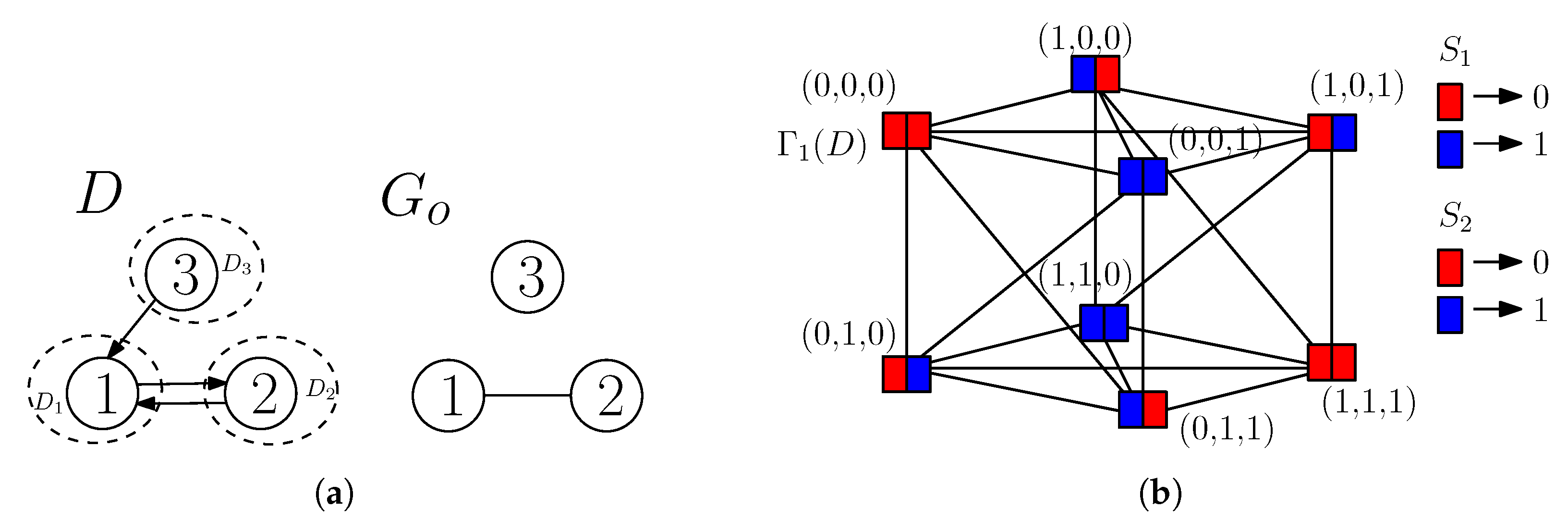
4.3. Proposed Confusion Graph Coloring for TSUIC

The confusion graph, which is only a function of the side-information graph, does not depend on the number of senders. Its coloring function described above for SSUIC may not lead to an index code for TSUIC because of the constraint due to the two senders. In this work, we propose a way of coloring the confusion graphs in TSUIC, which we call two-sender graph coloring. Before presenting a formal definition, we first define some notations that will be used in the remainder of this paper, unless stated otherwise.

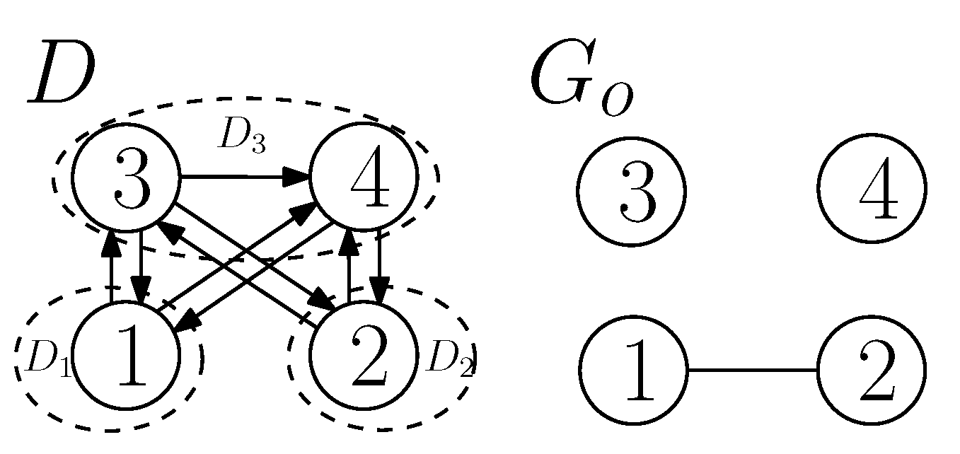
• Without loss of generality, we assume $x_1,x_2,\cdots ,x_{n_1}$ to be the messages requested by vertices in $V(D_1)$, $x_{n_1+1},x_{n_1+2},\cdots ,x_{n_1+n_2}$ the messages requested by vertices in $V(D_2)$, and $x_{n_1+n_2+1},x_{n_1+n_2+2},\cdots ,x_{n_1+n_2+n_3}$ the messages requested by vertices in $V(D_3)$ with $N=n_1+n_2+n_3$.
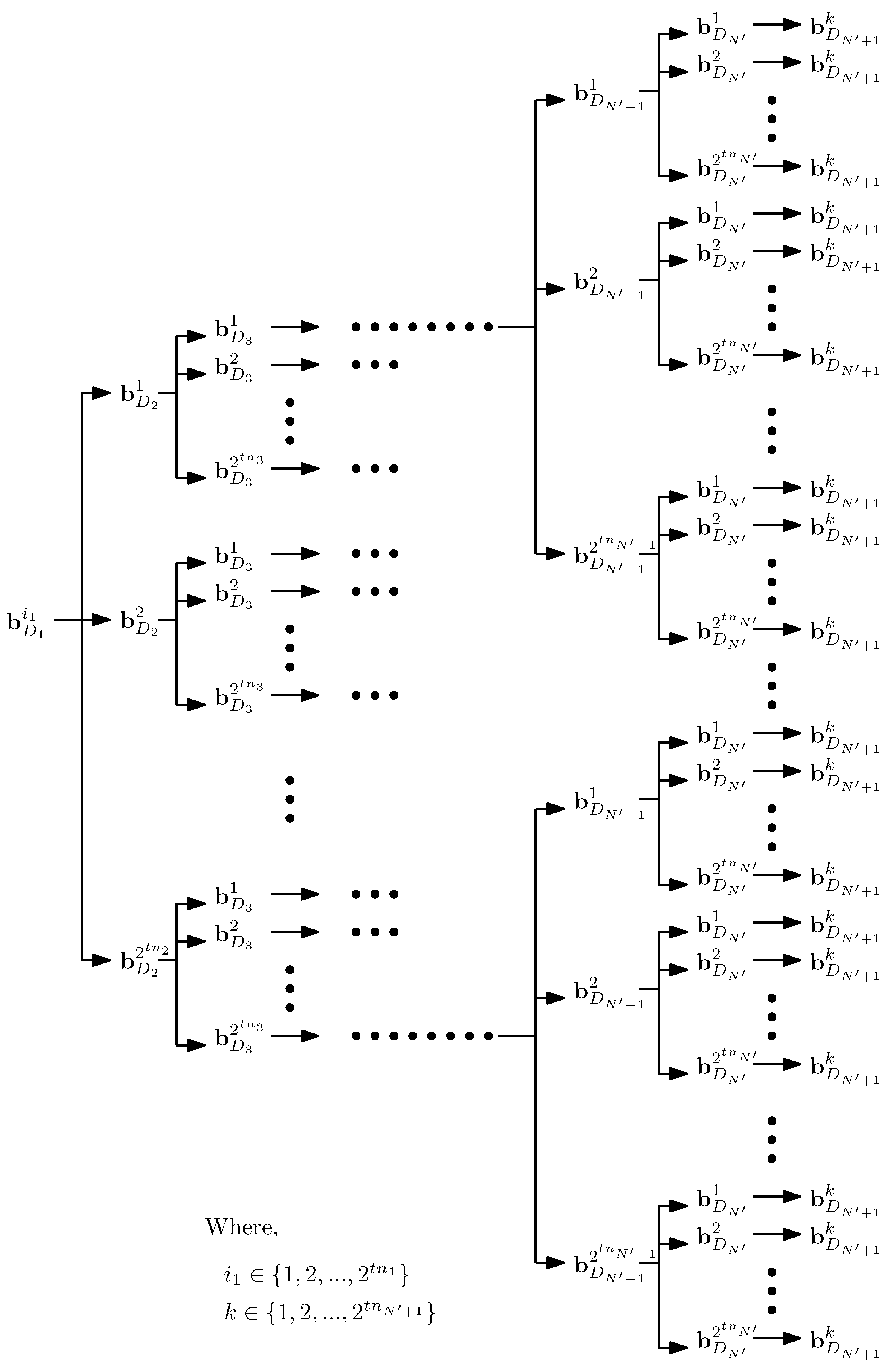
• Indices $i,i_1,i_2\in \{1,2,\cdots ,2^{t{n}_1}\}$, $j,j_1,j_2\in \{1,2,\cdots ,2^{t{n}_2}\}$ and $k,k_1,k_2\in \{1,2,\cdots ,2^{t{n}_3}\}$ are used in the representation of possible realizations of words of $t{n}_1$, $t{n}_2$ and $t{n}_3$ bits, respectively. For convenience, we use three indices (e.g., $i,i_1,i_2$) for the same set of numbers, where the first index (e.g., i) is used for a general case, and the remaining two indices (e.g., $i_1$ and $i_2$) are used to indicate any two words within the group of words.
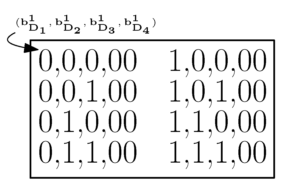
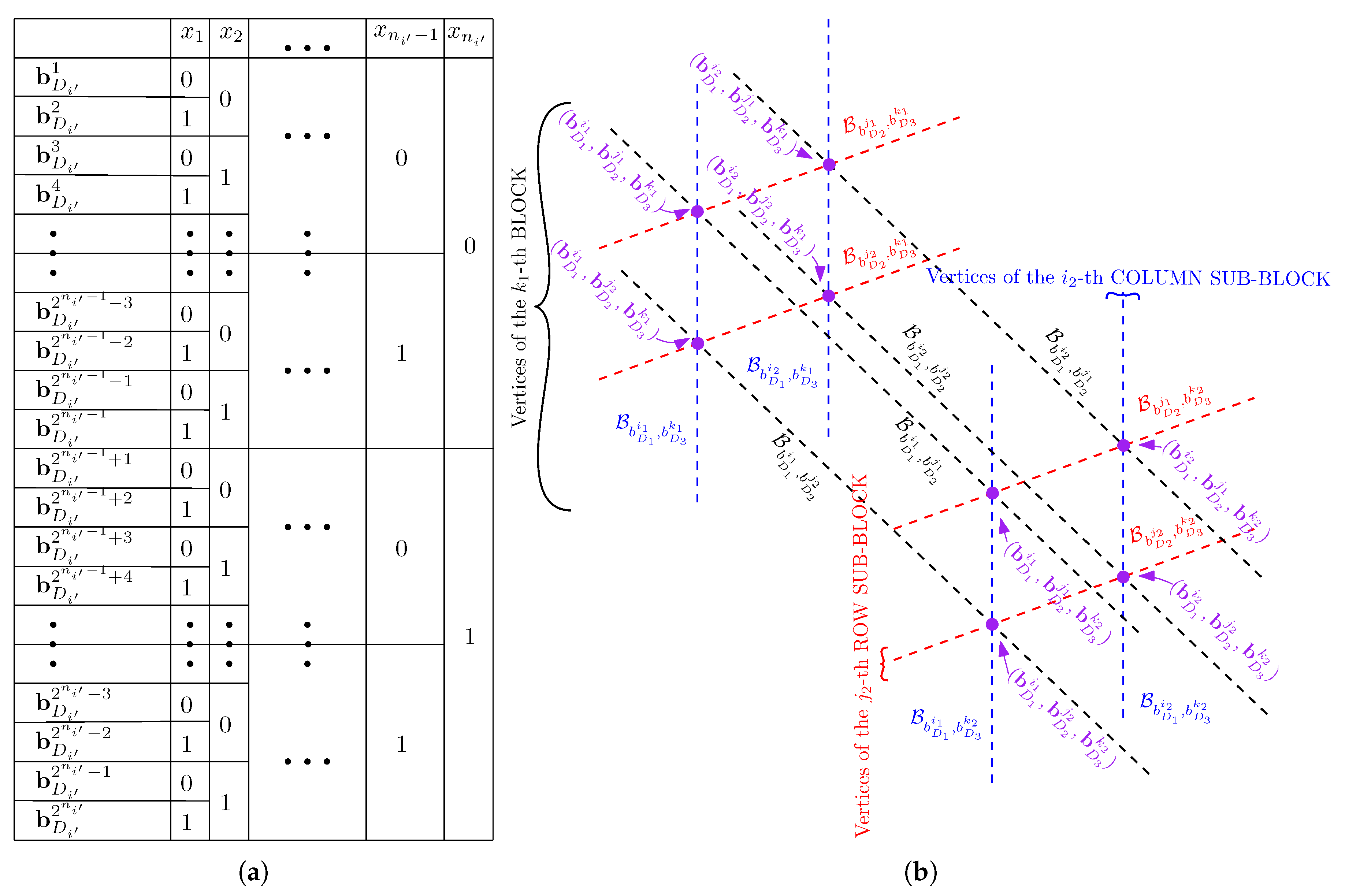
• We group the bits associated with the messages requested by vertices of $D_{i^{\prime }}$, $i^{\prime }\in \{1,2,3\}$. Within each group, each realization of the bits, i.e., each member in ${\{0,1\}}^{t{n}_{i^{\prime }}}$ is represented by a unique label ${\mathbf{b}}_{D_{i^{\prime }}}^{j^{\prime }}$, $j^{\prime }\in \{1,2,\cdots ,2^{t{n}_{i^{\prime }}}\}$. Figure A1a in Appendix A outlines each tuple ${\mathbf{b}}_{D_{i^{\prime }}}^{j^{\prime }}$ for $t=1$. Each message tuple $(x_1,\cdots ,x_N)$ realization can then be uniquely written as $({\mathbf{b}}_{D_1}^i,{\mathbf{b}}_{D_2}^j,{\mathbf{b}}_{D_3}^k)$ for some $i,j,k$.

Definition 8

(Two-sender graph coloring of ${\Gamma }_t(D)$). Let two onto functions $J_1:{\{0,1\}}^{t{n}_1}\times {\{0,1\}}^{t{n}_3}\to {\mathcal{J}}_1$, and $J_2:{\{0,1\}}^{t{n}_2}\times {\{0,1\}}^{t{n}_3}\to {\mathcal{J}}_2$ be the coloring functions carried out by senders $S_1$ and $S_2$, respectively. A proper two-sender graph coloring of ${\Gamma }_t(D)$ is an onto function $J_o:{\{0,1\}}^{t{n}_1}\times {\{0,1\}}^{t{n}_2}\times {\{0,1\}}^{t{n}_3}\to {\mathcal{J}}_1\times {\mathcal{J}}_2$ where $J_o(({\mathit{b}}_{D_1}^i,{\mathit{b}}_{D_2}^j,{\mathit{b}}_{D_3}^k))=(J_1({\mathit{b}}_{D_1}^i,{\mathit{b}}_{D_3}^k),J_2({\mathit{b}}_{D_2}^j,{\mathit{b}}_{D_3}^k))$ such that if $({\mathit{b}}_{D_1}^{i_1},{\mathit{b}}_{D_2}^{j_1},{\mathit{b}}_{D_3}^{k_1})$ and $({\mathit{b}}_{D_1}^{i_2},{\mathit{b}}_{D_2}^{j_2},{\mathit{b}}_{D_3}^{k_2})$ are adjacent vertices of ${\Gamma }_t(D)$, then $J_o(({\mathit{b}}_{D_1}^{i_1},{\mathit{b}}_{D_2}^{j_1},{\mathit{b}}_{D_3}^{k_1}))\ne J_o(({\mathit{b}}_{D_1}^{i_2},{\mathit{b}}_{D_2}^{j_2},{\mathit{b}}_{D_3}^{k_2}))$.

Remark 2.

The two-sender graph coloring is not a b-fold coloring that assigns a set of b colors to each vertex such that the color sets corresponding to two adjacent vertices do not share any color (refer to the definition of the fractional graph coloring [8]). In our definition, the color sets can share colors, as long as the color vectors (i.e., ordered pairs) are different.

4.4. A Few Lemmas for the TSUIC Confusion Graph Coloring

In the form of lemmas, we discuss two-sender graph coloring of ${\Gamma }_t(D)$ in detail. Before this, we first assume the following: For any indices $i^{\prime },j^{\prime }$, assume that $c_{i^{\prime }}$ and $c_{j^{\prime }}$ are any two distinct colors if $i^{\prime }\ne j^{\prime }$, and let $(c_{i^{\prime }},c_{j^{\prime }})$ be an ordered pair of colors. Any two ordered pairs of colors, $(c_{i_1^{\prime }},c_{j_1^{\prime }})$ and $(c_{i_2^{\prime }},c_{j_2^{\prime }})$, are said to be different (or not equal) if and only if $i_1^{\prime }\ne i_2^{\prime }$ or $j_1^{\prime }\ne j_2^{\prime }$ or both. If a color $c_{i^{\prime }}$ is associated with a sender $S_s$, $s\in \{1,2\}$, then we denote it by $c_{i^{\prime }}^s$.

In TSUIC, the two senders encode separately, so, in the aforementioned definition, we need to assign an ordered pair of colors for each vertex, where the first color is associated with $S_1$ and the second color with $S_2$. Now, we have the following lemmas.

Lemma 1.

For any two distinct vertices $u^N,v^N\in V({\Gamma }_t(D))$ that are labeled by $({\mathit{b}}_{D_1}^{i_1},{\mathit{b}}_{D_2}^j,{\mathit{b}}_{D_3}^k)$ and $({\mathit{b}}_{D_1}^{i_2},{\mathit{b}}_{D_2}^j,{\mathit{b}}_{D_3}^k)$, respectively, if $(u^N,v^N)\in E({\Gamma }_t(D))$, then we must have $J_o(u^N)=(c_{i_1^{\prime }}^1,c_{j_1^{\prime }}^2)$ and $J_o(v^N)=(c_{i_2^{\prime }}^1,c_{j_2^{\prime }}^2)$ such that $c_{i_1^{\prime }}^1\ne c_{i_2^{\prime }}^1$ and $c_{j_1^{\prime }}^2=c_{j_2^{\prime }}^2$ for some indices $i_1^{\prime },i_2^{\prime },j_1^{\prime },j_2^{\prime }$.

Proof. 

Since $(u^N,v^N)\in E({\Gamma }_t(D))$, $u^N$ and $v^N$ are confusable. Moreover, these two tuples are confusable only at some vertex in $V(D_1)$. This is because the labels $({\mathbf{b}}_{D_1}^{i_1},{\mathbf{b}}_{D_2}^j,{\mathbf{b}}_{D_3}^k)$ and $({\mathbf{b}}_{D_1}^{i_2},{\mathbf{b}}_{D_2}^j,{\mathbf{b}}_{D_3}^k)$ of $u^N$ and $v^N$, respectively, are different only in ${\mathbf{b}}_{D_1}^i$ sub-label (which is representing $t{n}_1$-bit tuples of the messages requested by vertices in $V(D_1)$). Now, for the sender $S_2$, which does not contain any message in ${\mathcal{P}}_1$ (messages requested by receivers in $V(D_1)$), the coloring function $J_2({\mathbf{b}}_{D_2}^j,{\mathbf{b}}_{D_3}^k)$ provides the same color to both vertices. Thus, $c_{j_1^{\prime }}^2=c_{j_2^{\prime }}^2$. On the other hand, for the sender $S_1$, which contains all messages in ${\mathcal{P}}_1$, it is necessary to have $J_1({\mathbf{b}}_{D_1}^{i_1},{\mathbf{b}}_{D_3}^k)\ne J_1({\mathbf{b}}_{D_1}^{i_2},{\mathbf{b}}_{D_3}^k)$ because these two tuples $({\mathbf{b}}_{D_1}^{i_1},{\mathbf{b}}_{D_3}^k)$ and $({\mathbf{b}}_{D_1}^{i_2},{\mathbf{b}}_{D_3}^k)$ are confusable given that $({\mathbf{b}}_{D_1}^{i_1},{\mathbf{b}}_{D_2}^j,{\mathbf{b}}_{D_3}^k)$ and $({\mathbf{b}}_{D_1}^{i_2},{\mathbf{b}}_{D_2}^j,{\mathbf{b}}_{D_3}^k)$ are confusable at some receiver in $V(D_1)$. Thus, $c_{i_1^{\prime }}^1\ne c_{i_2^{\prime }}^1$. □

In a similar reasoning as in the above proof (of Lemma 1), one can prove the following lemma:

Lemma 2.

For any two distinct vertices, $u^N,v^N\in V({\Gamma }_t(D))$ such that they are labeled by $({\mathit{b}}_{D_1}^i,{\mathit{b}}_{D_2}^{j_1},{\mathit{b}}_{D_3}^k)$ and $({\mathit{b}}_{D_1}^i,{\mathit{b}}_{D_2}^{j_2},{\mathit{b}}_{D_3}^k)$, respectively, if $(u^N,v^N)\in E({\Gamma }_t(D))$, then we must have $J_o(u^N)=(c_{i_1^{\prime }}^1,c_{j_1^{\prime }}^2)$ and $J_o(v^N)=(c_{i_2^{\prime }}^1,c_{j_2^{\prime }}^2)$ such that $c_{i_1^{\prime }}^1=c_{i_2^{\prime }}^1$ and $c_{j_1^{\prime }}^2\ne c_{j_2^{\prime }}^2$ for some indices $i_1^{\prime },i_2^{\prime },j_1^{\prime },j_2^{\prime }$.

If $u^N$ and $v^N$ are confusable at some vertices in $V(D_1)$ and in $V(D_2)$, then referring to Lemmas 1 and 2, we get the following:

Lemma 3.

For any two distinct vertices, $u^N,v^N\in V({\Gamma }_t(D))$ such that they are labeled by $({\mathit{b}}_{D_1}^{i_1},{\mathit{b}}_{D_2}^{j_1},{\mathit{b}}_{D_3}^k)$ and $({\mathit{b}}_{D_1}^{i_2},{\mathit{b}}_{D_2}^{j_2},{\mathit{b}}_{D_3}^k)$, respectively, if $(u^N,v^N)\in E({\Gamma }_t(D))$ due to confusion at some vertices in $V(D_1)$ and in $V(D_2)$, then we must have $J_o(u^N)=(c_{i_1^{\prime }}^1,c_{j_1^{\prime }}^2)$ and $J_o(v^N)=(c_{i_2^{\prime }}^1,c_{j_2^{\prime }}^2)$ such that $c_{i_1^{\prime }}^1\ne c_{i_2^{\prime }}^1$ and $c_{j_1^{\prime }}^2\ne c_{j_2^{\prime }}^2$ for some indices $i_1^{\prime },i_2^{\prime },j_1^{\prime },j_2^{\prime }$.

If $u^N$ and $v^N$ are confusable at some vertices in $V(D_3)$, then whilst coloring ${\Gamma }_t(D)$ in two-sender graph coloring, it suffices to have a different color associated with any one of the senders because all the messages in ${\mathcal{P}}_3$ are contained by both senders $S_1$ and $S_2$. Thus, we have the following lemma:

Lemma 4.

For any two vertices, $u^N,v^N\in V({\Gamma }_t(D))$ such that they are labeled by $({\mathit{b}}_{D_1}^i,{\mathit{b}}_{D_2}^j,{\mathit{b}}_{D_3}^{k_1})$ and $({\mathit{b}}_{D_1}^i,{\mathit{b}}_{D_2}^j,{\mathit{b}}_{D_3}^{k_2})$, respectively, if $(u^N,v^N)\in E({\Gamma }_t(D))$, then we have $J_o(u^N)=(c_{i_1^{\prime }}^1,c_{j_1^{\prime }}^2)$ and $J_o(v^N)=(c_{i_2^{\prime }}^1,c_{j_2^{\prime }}^2)$ such that either $c_{i_1^{\prime }}^1\ne c_{i_2^{\prime }}^1$, or $c_{j_1^{\prime }}^2\ne c_{j_2^{\prime }}^2$, or both.

5. The Optimal Broadcast Rate for TSUIC

For a TSUIC problem with t-bit messages, we have the following theorem:

Theorem 2.

The optimal broadcast rate for a TSUIC problem with t-bit messages is

$${\beta }_t(D,G_o)=\underset{J_1,J_2}{\min }\frac{\lceil {\log }_2|{\mathcal{J}}_1|\rceil +\lceil {\log }_2|{\mathcal{J}}_2|\rceil }{t}.$$

(2)

Proof. 

For $s\in \{1,2\}$, consider $J_s$, a coloring function of the sender $S_s$, with a set of colors ${\mathcal{J}}_s$. A two-sender index code is obtained by $S_1$ mapping distinct colors in ${\mathcal{J}}_1$ to distinct sub-codewords, and $S_2$ mapping distinct colors in ${\mathcal{J}}_2$ to distinct sub-codewords. By definition, all confusable vertex pairs are assigned different codewords. Now, for $s\in \{1,2\}$, the sender $S_s$ transmits $|{\mathcal{J}}_s|$ sub-codewords. Equivalently, $\lceil {\log }_2\left|{\mathcal{J}}_s\right|\rceil$ bits are transmitted by $S_s$. This is because the number of bits required to index $|{\mathcal{J}}_s|$ colors are $\lceil {\log }_2\left|{\mathcal{J}}_s\right|\rceil$. Minimizing the sum $(\lceil {\log }_2|{\mathcal{J}}_1|\rceil +\lceil {\log }_2|{\mathcal{J}}_2|\rceil )$ over all coloring functions $J_1$ (of $S_1$) and $J_2$ (of $S_2$) per received message bits (i.e., t), we get

$${\beta }_t(D,G_o)\le \underset{J_1,J_2}{\min }\frac{\lceil {\log }_2|{\mathcal{J}}_1|\rceil +\lceil {\log }_2|{\mathcal{J}}_2|\rceil }{t}.$$

(3)

From the definition of ${\beta }_t(D,G_o)$, we have ${\beta }_t(D,G_o)=\underset{\mathcal{E}}{\min }\frac{p_1+p_2}{t}$, so there exists a two-sender index code such that $S_1$ and $S_2$ transmit $p_1^{\prime }$-bit and $p_2^{\prime }$-bit sub-codewords, respectively, resulting in

$${\beta }_t(D,G_o)=\frac{p_1^{\prime }+p_2^{\prime }}{t}.$$

(4)

Now, for each sender $S_s$, we know that there are at most $2^{p_s^{\prime }}$ possible sub-codewords. Consider a bijective function that maps each sub-codeword to a color. A valid code must translate to a valid two-sender graph coloring. Thus, there exists a valid two-sender graph coloring such that $|{\mathcal{J}}_1^{\prime }|\le 2^{p_1^{\prime }}$ and $|{\mathcal{J}}_2^{\prime }|\le 2^{p_2^{\prime }}$, or, equivalently, $p_1^{\prime }\ge \lceil {\log }_2|{\mathcal{J}}_1^{\prime }|\rceil$ and $p_2^{\prime }\ge \lceil {\log }_2|{\mathcal{J}}_2^{\prime }|\rceil$ as both are non-negative integers. Substituting the inequalities of $p_1^{\prime }$ and $p_2^{\prime }$ in (4), we get

$${\beta }_t(D,G_o)\ge \frac{\lceil {\log }_2|{\mathcal{J}}_1^{\prime }|\rceil +\lceil {\log }_2|{\mathcal{J}}_2^{\prime }|\rceil }{t}.$$

(5)

Now, we prove equality in (3). This is done by contradiction. Suppose that

$${\beta }_t(D,G_o)<\underset{J_1,J_2}{\min }\frac{\lceil {\log }_2|{\mathcal{J}}_1|\rceil +\lceil {\log }_2|{\mathcal{J}}_2|\rceil }{t}.$$

(6)

From (5) and (6), we get

$$\frac{\lceil {\log }_2|{\mathcal{J}}_1^{\prime }|\rceil +\lceil {\log }_2|{\mathcal{J}}_2^{\prime }|\rceil }{t}<\underset{J_1,J_2}{\min }\frac{\lceil {\log }_2|{\mathcal{J}}_1|\rceil +\lceil {\log }_2|{\mathcal{J}}_2|\rceil }{t},$$

(7)

and this leads to a contradiction. Thus, ${\beta }_t(D,G_o)=\underset{J_1,J_2}{\min }\frac{\lceil {\log }_2|{\mathcal{J}}_1|\rceil +\lceil {\log }_2|{\mathcal{J}}_2|\rceil }{t}$. □

We illustrate two-sender graph coloring of a confusion graph in TSUIC, and a mapping function that maps colors to codewords at each sender from the following example.

Example 1.

Consider a TSUIC problem $(D,G_o)$ of the following: $(1|2),(2|1),(3|1)$, and ${\mathcal{M}}_1=\{1,3\}$, ${\mathcal{M}}_2=\{2,3\}$ with $t=1$. The problem is depicted in Figure 4a. We have $V(D_1)=\left\{1\right\}$, $V(D_2)=\left\{2\right\}$, $V(D_3)=\left\{3\right\}$, and $N=3$. The confusion graph ${\Gamma }_1(D)$ has $2^N=8$ vertices labeled by all possible realizations of a word with three bits. In ${\Gamma }_1(D)$, any two vertices are connected by an edge if the message tuples labeling the vertices are confused at some receiver. For example, $(0,0,0)$ and $(1,0,0)$ are connected by an edge because these two message tuples are confused at receiver 1. The confusion graph ${\Gamma }_1(D)$ is depicted in Figure 4b. Now, we perform two-sender graph coloring of the vertices of ${\Gamma }_1(D)$. In two-sender graph coloring, each vertex of ${\Gamma }_1(D)$ is assigned with an ordered pair of colors; the first color is always associated with $S_1$ and the second color is always associated with $S_2$, and we color the vertices as dictated by Lemmas 1–4. For example, consider $(0,0,0)$ and $(1,0,0)$. These two tuples are confused at receiver 1 (requesting $x_1$). As $S_2$, which does not know $x_1$, the tuples $(0,0,0)$ and $(1,0,0)$, which have the same second and third message bits, are treated as the same. Thus, $S_2$ must assign the same color, say RED, to both the tuples. As $S_1$ knows $x_1$ and the tuples are confusable at receiver 1, it must assign two different colors, say RED and BLUE, to $(0,0,0)$ and $(1,0,0)$, respectively. In a similar way, we assign ordered pairs of colors to all vertices of ${\Gamma }_1(D)$ as shown in Figure 4b. Altogether, one can get ${\mathcal{J}}_1=\{\mathrm{RED},\mathrm{BLUE}\}$ and ${\mathcal{J}}_2=\{\mathrm{RED},\mathrm{BLUE}\}$. Now, we assume a mapping function that maps RED to 0 and BLUE to 1. Thus, we get $(0,0,0)\to 00$, $(1,0,0)\to 10$, $(0,1,0)\to 01$ and so on for the remaining tuples (vertices of ${\Gamma }_t(D)$). Thus, $\{00,10,01,11\}$ are codewords of a valid two-sender index code for $(D,G_o)$, where each sender transmits a 1-bit sub-codeword for a message tuple, and the sum of bits to be transmitted by the two senders is two for each message tuple. Consequently, ${\beta }_t(D,G_o)\le 2$. Each sender has one private message, and that must be transmitted by that sender, so there must be at least one transmission by that sender. Thus, ${\beta }_t(D,G_o)\ge 2$. Altogether, we get ${\beta }_t(D,G_o)=2$.

5.1. Lower Bounds

For any D, we have $\beta (D)\le {\beta }_t(D)$ for all t (by definition). Since any index code for $(D,G_o)$ is also an index code for D, but the converse is not always true, so we have the following:

Lemma 5 (A simple lower bound).

For any D and $G_o$, $\beta (D,G_o)\ge \beta (D)$.

In TSUIC, each sender $S_s$ transmits at least $\beta (D_s)$, for $s\in \{1,2\}$. We now provide a lower bound of the optimal broadcast rate for a TSUIC problem with t-bit messages in the following lemma.

Lemma 6 (A lower bound).

For any two-sender index-coding problem $(D,G_o)$, ${\beta }_t(D,G_o)\ge {\beta }_t(D_1)+{\beta }_t(D_2)$, and $\beta (D,G_o)\ge \beta (D_1)+\beta (D_2)$.

Proof. 

For any two-sender index-coding problem $(D,G_o)$, let $(D^{\prime },G_o^{\prime })$ be its sub-problem induced by vertices $V(D_1)\cup V(D_2)$. Observe that $V(D^{\prime })\cap V(D_3)=\varnothing$. Now, we have ${\beta }_t(D^{\prime },G_o^{\prime })={\beta }_t(D_1)+{\beta }_t(D_2)$ ([17], Th. 1). For any index-coding problem, its broadcast rate is always lower bounded by the broadcast rate of any sub-problem, so we get

$${\beta }_t(D,G_o)\ge {\beta }_t(D^{\prime },G_o^{\prime })={\beta }_t(D_1)+{\beta }_t(D_2).$$

(8)

We know that $\underset{t\to \infty }{\lim }{\beta }_t(D_1)=\beta (D_1)$, $\underset{t\to \infty }{\lim }{\beta }_t(D_2)=\beta (D_2)$ and $\beta (D,G_o)=\underset{t\to \infty }{\lim }{\beta }_t(D,G_o)$ (by Definition 3). Now, taking a limit $t\to \infty$ on both sides in (8), we get

$$\begin{array}{cc}\hfill \beta (D,G_o)& \ge \beta (D_1)+\beta (D_2).\hfill \end{array}$$

(9)

□

To compute the simple lower bound to the optimal broadcast rate of a given problem in TSUIC, we utilize the following SSUIC results by Arbabjolfaei and Kim ([8], Prop. 3, Th. 2, Th. 3).

Theorem 3.

In SSUIC, for a side-information digraph D having two sub-digraphs $D_a$ and $D_b$ induced by vertices $V(D_a)$ and $V(D_b)$, respectively, such that $V(D_a)\cup V(D_b)=V(D)$ and $V(D_a)\cap V(D_b)=\varnothing$, we have

(i) 

$\beta (D)=\beta (D_a)+\beta (D_b)$ if there is (i) no interaction between $D_a$ and $D_b$ (i.e., no $D_a\to D_b$ and $D_b\to D_a$), or (ii) a one-way interaction (either partially or fully participated) between $D_a$ and $D_b$, i.e., either $D_a\to D_b$ or $D_b\to D_a$, but not both and

(ii) 

$\beta (D)=\mathit{max}\{\beta (D_a),\beta (D_b)\}$ if there is a fully participated both way interaction between $D_a$ and $D_b$ (i.e., fully participated $D_a\rightleftarrows D_b$).

5.2. Optimal Broadcast Rates for CASE I and CASE II-A: The Arcs between $D_1$, $D_2$ and $D_3$ Are Not Critical in Asymptotic Regime in the Message Size

For a digraph D whose $f(D)$ belongs to a digraph of CASE I and CASE II-A (see Figure 3), we have the following results.

Theorem 4 (CASE I).

For any D having any interaction (i.e., either fully participated or partially participated) between its sub-digraphs $D_1$, $D_2$ and $D_3$, if $f(D)\in \{{\mathrm{H}}_1,{\mathrm{H}}_2,\cdots ,{\mathrm{H}}_{14}\}$ (i.e., a digraph H of CASE I in Figure 3), then $\beta (D,G_o)=\beta (D_1)+\beta (D_2)+\beta (D_3)=\beta (D)$.

Proof. 

Referring to the definition of the mapping function f (in Section 3), we know that for any D if $f(D)\in \{{\mathrm{H}}_1,{\mathrm{H}}_2,\cdots ,{\mathrm{H}}_{14}\}$, then the interaction between $D_1$, $D_2$ and $D_3$ of D are acyclic. Thus, one can arrange $D_1$, $D_2$ and $D_3$ in a sequence such that there is no arc between $D_1$, $D_2$ and $D_3$ in a backward direction. Without loss of generality, let the sequence be $D_1$, $D_2$ and $D_3$. Now for D, referring to Theorem 3, we get

$$\beta (D)=\beta (D_1\cup D_2)+\beta (D_3)=\beta (D_1)+\beta (D_2)+\beta (D_3).$$

(10)

From Lemma 5, we have

$$\beta (D,G_o)\ge \beta (D).$$

(11)

Now from (10) and (11), we get

$$\beta (D,G_o)\ge \beta (D_1)+\beta (D_2)+\beta (D_3).$$

(12)

In TSUIC, if we consider the sub-digraphs $D_1$, $D_2$ and $D_3$ separately, then their respective source constraint graphs are the sub-graphs of $G_0$ induced by vertices $V(D_1)$, $V(D_2)$ and $V(D_3)$, denoted $G_0^1$, $G_0^2$ and $G_0^3$, respectively. These sub-graphs are edgeless graphs, and thus one can get $\beta (D_1,G_0^1)=\beta (D_1)$, $\beta (D_2,G_0^2)=\beta (D_2)$ and $\beta (D_3,G_0^3)=\beta (D_3)$. We know that the optimal broadcast rate of a side-information digraph is always less than or equal to the sum of the optimal broadcast rates of its sub-digraphs, so

$$\begin{array}{cc}\hfill \beta (D,G_o)& \le \beta (D_1,G_0^1)+\beta (D_2,G_0^2)+\beta (D_3,G_0^3)\hfill \\ & \le \beta (D_1)+\beta (D_2)+\beta (D_3).\hfill \end{array}$$

(13)

From (10), (12) and (13), we get $\beta (D,G_o)=\beta (D_1)+\beta (D_2)+\beta (D_3)=\beta (D)$. □

Example 2.

Consider a TSUIC problem of the following: $(1),(2|1,4,5),(3|1,2,4,5),(4|1,5),(5|1,4)$, and ${\mathcal{M}}_1=\{1,4,5\}$, ${\mathcal{M}}_2=\{1,2,3\}$. We compute its $\beta (D,G_o)$ using Theorem 4. Refer to Figure 5 for details.

Proposition 1.

For any D having a fully-participated interaction between its sub-digraphs $D_1$, $D_2$ and $D_3$, if $f(D)\in \{{\mathrm{H}}_1,{\mathrm{H}}_{16}\}$, then ${\beta }_t(D,G_o)={\beta }_t(D_1)+{\beta }_t(D_2)+{\beta }_t(D_3)+ϵ/t$ for some $ϵ\in \{-2,-1,0\}$.

Proof. 

Refer to Appendix C. □

Definition 9 (Vertex-transitive graphs).

An undirected graph G is vertex-transitive if for every pair $u,v\in V(G)$ there exists an automorphism mapping from u to v. In the automorphism mapping of all vertices in $V(G)$, the graph is mapped onto itself whilst preserving the connectivity of the vertices and edges.

Remark 3.

The proof of the Proposition 1 is based on the analysis of the confusion graph ${\Gamma }_t(D)$ and its coloring. This is described in Section 4. As a confusion graph possesses some symmetry within—in fact, all confusion graphs are vertex-transitive—whilst analyzing them (especially coloring), we systematically group its vertices and then analyze the graph based on these groups (rather than individual vertices). This way, for a TSUIC problem whose sub-problems interact with each other in some way, we can reduce the complexity arising during its analysis (especially finding the number of colors in a proper coloring of ${\Gamma }_t(D)$) due to the number of vertices, which is exponential in t and N. The proposed grouping of the vertices of the confusion graph and its characteristics are stated in Appendix B.

Theorem 5 (CASE I and CASE II-A).

For any D having any interaction (i.e., either fully participated or partially participated) between its sub-digraphs $D_1$, $D_2$ and $D_3$, if $f(D)\in \{{\mathrm{H}}_1,{\mathrm{H}}_2,\cdots ,{\mathrm{H}}_{17}\}\backslash \{{\mathrm{H}}_8,{\mathrm{H}}_9,\cdots ,{\mathrm{H}}_{14}\}$, then ${\beta }_t(D,G_o)={\beta }_t(D_1)+{\beta }_t(D_2)+{\beta }_t(D_3)+ϵ/t$, where $ϵ\in \{-2,-1,0\}$, and $\beta (D,G_o)=\beta (D_1)+\beta (D_2)+\beta (D_3)$.

Proof. 

For convenience, let $D=D^i$ if $f(D)={\mathrm{H}}_i$. Now, for $D^i$, $i\in \{1,16\}$, with a fully-participated interaction between the sub-digraphs, we have the following from Proposition 1:

$$\begin{array}{c}\hfill {\beta }_t(D^i,G_o)={\beta }_t(D_1)+{\beta }_t(D_2)+{\beta }_t(D_3)+ϵ/t,\end{array}$$

(14)

for some $ϵ\in \{-2,-1,0\}$. For any $D^i$, $i\in \{1,2,3,\cdots ,17\}$, having either a partially-participated or a fully-participated interaction between the sub-digraphs, we have the following observations: The interactions between the sub-digraphs (i.e., $D_1$, $D_2$ and $D_3$) are equal to or more than that in $D^1$, so

$${\beta }_t(D^i,G_o)\le {\beta }_t(D^1,G_o)$$

(15)

and equal to or fewer than that in $D^{14}$ (with a fully-participated interaction between the sub-digraphs), so

$${\beta }_t(D^i,G_o)\ge {\beta }_t(D^{14},G_o).$$

(16)

Now, from (14)–(16), we get

$${\beta }_t(D^i,G_o)={\beta }_t(D,G_o)={\beta }_t(D_1)+{\beta }_t(D_2)+{\beta }_t(D_3)+ϵ/t,$$

(17)

where $ϵ\in \{-2,-1,0\}$ and $i\in \{1,2,\cdots ,17\}\backslash \{{\mathrm{H}}_8,{\mathrm{H}}_9,\cdots ,{\mathrm{H}}_{14}\}$.

Now, taking a limit $t\to \infty$ on both sides in (17), we get

$$\begin{array}{cc}\hfill \beta (D,G_o)=\underset{t\to \infty }{\lim }{\beta }_t(D,G_o)& =\underset{t\to \infty }{\lim }({\beta }_t(D_1)+{\beta }_t(D_2)+{\beta }_t(D_3)+ϵ/t)\hfill \\ & =\beta (D_1)+\beta (D_2)+\beta (D_3),\hfill \end{array}$$

(18)

where $\underset{t\to \infty }{\lim }\frac{ϵ}{t}=0$. □

Remark 4.

For any D having non-empty $D_1$, $D_2$ and $D_3$ with fully-participated interactions between them such that $f(D)\in \{{\mathrm{H}}_{15},{\mathrm{H}}_{16},{\mathrm{H}}_{17}\}$, in SSUIC, we have $\beta (D)=\beta (D_3)+\max \{\beta (D_1),\beta (D_2)\}$ by Theorem 3; however, in TSUIC, $\beta (D)$, a lower bound to $\beta (D,G_o)$, is not achievable due to Theorem 5.

Corollary 1.

For any D having any interaction (i.e., either fully participated or partially participated) between its sub-digraphs $D_1$, $D_2$ and $D_3$, if $f(D)\in \{{\mathrm{H}}_1,{\mathrm{H}}_2,\cdots ,{\mathrm{H}}_{17}\}$, then the arcs (contributing to that interaction) between $D_1$, $D_2$ and $D_3$ of D are not critical in TSUIC in the asymptotic regime in message size (considering infinitely long messages).

Proof. 

The proof follows from Theorems 4 and 5. □

5.3. Optimal Broadcast Rates for CASE II-B

Theorem 6 (CASE II-B).

For any D having a fully participated interaction between its sub-digraphs $D_1$, $D_2$ and $D_3$, and t-bit messages for any $t\ge 1$, if $f(D)\in \{{\mathrm{H}}_{18},{\mathrm{H}}_{19},{\mathrm{H}}_{20}\}$, then ${\beta }_t(D,G_o)=\max \{{\beta }_t(D_3),{\beta }_t(D_1)+{\beta }_t(D_2)\}$ and $\beta (D,G_o)=\max \{\beta (D_3),\beta (D_1)+\beta (D_2)\}$.

Proof. 

Refer to Appendix D. □

Corollary 2.

For any D having a fully participated interaction between its sub-digraphs $D_1$, $D_2$ and $D_3$ such that $f(D)\in \{{\mathrm{H}}_{18},{\mathrm{H}}_{20}\}$, $\beta (D,G_o)=\beta (D)$.

Proof. 

The result follows from Theorems 3 and 6. □

Remark 5.

In TSUIC, for any D having a fully participated interaction between its non-empty sub-digraphs $D_1$, $D_2$ and $D_3$ such that $f(D)={\mathrm{H}}_{19}$, no TSUIC scheme achieves $\beta (D)$ if $\beta (D_3)<\beta (D_1)+\beta (D_2)$ because $\beta (D)=\max \{\beta (D_1),\beta (D_2),\beta (D_3)\}\}$ (by Theorem 3) and $\beta (D,G_o)$ is at least $\beta (D_1)+\beta (D_2)$ (by Lemma 6).

Example 3.

Consider a TSUIC problem of the following: $(1|3,4),(2|3,4),(3|1,2,4),(4|1,2)$, and ${\mathcal{M}}_1=\{1,3,4\}$, ${\mathcal{M}}_2=\{2,3,4\}$. We compute its $\beta (D,G_o)$ and ${\beta }_t(D,G_o)$ using Theorem 6. Refer to Figure 6 for details.

5.4. Optimal Broadcast Rates for CASE II-C: An Upper Bound, and Special Cases Where the Upper Bound Is Tight

Theorem 7 (CASE II-C).

For any D having a fully participated interaction between its sub-digraphs $D_1$, $D_2$ and $D_3$, and t-bit messages for any $t\ge 1$, if $f(D)\in \{{\mathrm{H}}_{21},{\mathrm{H}}_{22},\cdots ,{\mathrm{H}}_{32}\}$, then

(i) 

${\beta }_t(D,G_o)\le {\beta }_t(D_2)+\mathit{max}\{{\beta }_t(D_1),{\beta }_t(D_3)\}$,

(ii) 

${\beta }_t(D,G_o)={\beta }_t(D_1)+{\beta }_t(D_2)$ if ${\beta }_t(D_1)\ge {\beta }_t(D_3)$,

(iii) 

$\beta (D,G_o)\le \beta (D_2)+\mathit{max}\{\beta (D_1),\beta (D_3)\}$, and

(iv) 

$\beta (D,G_o)=\beta (D_1)+\beta (D_2)$ if $\beta (D_1)\ge \beta (D_3)$.

Proof. 

Refer to Appendix E. □

Case $(iii)$ in Theorem 7 can be strengthened as follows:

Proposition 2 (CASE II-C).

For any D having a fully participated interaction between its sub-digraphs $D_1$, $D_2$ and $D_3$ such that $f(D)\in \{{\mathrm{H}}_{21},{\mathrm{H}}_{22},\cdots ,{\mathrm{H}}_{32}\}$, $\beta (D,G_o)=\beta (D_2)+\max \{\beta (D_1),\beta (D_3)\}$.

Proof. 

It follows from Theorem 7 that $\beta (D,G_o)=\beta (D_1)+\beta (D_2)$ if $\beta (D_1)\ge \beta (D_3)$, and for the case when $\beta (D_1)\le \beta (D_3)$,

$$\beta (D,G_o)\le \beta (D_2)+\beta (D_3).$$

(19)

For D whose $f(D)\in \{{\mathrm{H}}_{21},{\mathrm{H}}_{22},\cdots ,{\mathrm{H}}_{32}\}\backslash \{{\mathrm{H}}_{28},{\mathrm{H}}_{29}\}$ (all digraphs of CASE II-C except ${\mathrm{H}}_{28}$ and ${\mathrm{H}}_{29}$), considering Theorem 3, we get $\beta (D)=\beta (D_2)+\beta (D_3)$ if $\beta (D_1)\le \beta (D_3)$. As $\beta (D)\le \beta (D,G_o)$ (Lemma 5), so

$$\beta (D,G_o)\ge \beta (D_2)+\beta (D_3).$$

(20)

The interaction among $D_1$, $D_2$ and $D_3$ in $D^{28}$ (that is, D where $f(D)={\mathrm{H}}_{28}$) is less than that in $D^{32}$. Thus,

$$\beta (D^{28},G_o)\ge \beta (D^{32},G_o).$$

(21)

From (20) and (21), we get

$$\beta (D^{28},G_o)\ge \beta (D^{32},G_o)\ge \beta (D_2)+\beta (D_3),$$

(22)

if $\beta (D_1)\le \beta (D_3)$. Due to the similar aforementioned reasoning, we get

$$\beta (D^{29},G_o)\ge \beta (D^{31},G_o)\ge \beta (D_2)+\beta (D_3).$$

(23)

From (19), (20), (22) and (23), we get $\beta (D,G_o)=\beta (D_2)+\beta (D_3)$ if $\beta (D_1)\le \beta (D_3)$ for any D with $f(D)\in \{{\mathrm{H}}_{21},{\mathrm{H}}_{22},\cdots ,{\mathrm{H}}_{32}\}$. Altogether, $\beta (D,G_o)=\beta (D_2)+\max \{\beta (D_1),\beta (D_3)\}$. □

Corollary 3.

For any D having a fully participated interaction between its sub-digraphs $D_1$, $D_2$ and $D_3$ such that $f(D)\in \{{\mathrm{H}}_{21},{\mathrm{H}}_{22},\cdots ,{\mathrm{H}}_{27}\}$, $\beta (D,G_o)=\beta (D)$.

Proof. 

For the given digraph D, by applying Theorem 3, one can get $\beta (D)=\beta (D_2)+\max \{\beta (D_1),\beta (D_3)\}$, and this equals $\beta (D,G_o)$ by Proposition 2. □

Corollary 4.

For any D such that $f(D)\in \{{\mathrm{H}}_{30},{\mathrm{H}}_{31},{\mathrm{H}}_{32}\}$,

(i) 

if $\beta (D_1)\le \beta (D_3)$, then $\beta (D,G_o)=\beta (D_2)+\beta (D_3)=\beta (D)$,

(ii) 

if $\beta (D_1)>\beta (D_3)$, then

(a) 

if $\beta (D_1)\ge \beta (D_2)+\beta (D_3)$, then $\beta (D,G_o)=\beta (D_1)+\beta (D_2)\ge \beta (D_1)=\beta (D)$, with a strict inequality if $D_2$ is non-empty, and

(b) 

if $\beta (D_1)\le \beta (D_2)+\beta (D_3)$, then $\beta (D,G_o)=\beta (D_1)+\beta (D_2)>\beta (D_2)+\beta (D_3)=\beta (D)$ for a non-empty $D_2$.

Proof. 

If $\beta (D_1)\le \beta (D_3)$, then $\beta (D_1)\le \beta (D_3)+\beta (D_2)$. Now, from Proposition 2 and Theorem 3, $\beta (D,G_o)=\beta (D_2)+\beta (D_3)=\beta (D)$. For the case $\beta (D_1)>\beta (D_3)$, the results directly follow from Proposition 2 and Theorem 3. □

Remark 6.

Let $D=D^i$ if $f(D)={\mathrm{H}}_i$. Now, for any D such that $f(D)\in \{{\mathrm{H}}_{28},{\mathrm{H}}_{29}\}$, we have the following if $\beta (D_1)\le \beta (D_3)$:

(i) 

$\{\beta (D^{32},G_o)=\beta (D^{32})=\beta (D_2)+\beta (D_3)\}\le \beta (D^{28})\le \beta (D^{28},G_o)\le \{\beta (D^{26})=\beta (D^{26},G_o)=\beta (D_2)+\beta (D_3)\}$ from Proposition 2, Theorem 3, Corollarys 3 and 4, and Lemma 5. This implies $\beta (D^{28})=\beta (D^{28},G_o)=\beta (D_2)+\beta (D_3)$.

(ii) 

$\{\beta (D^{31},G_o)=\beta (D^{31})=\beta (D_2)+\beta (D_3)\}\le \beta (D^{29})\le \beta (D^{29},G_o)\le \{\beta (D^{27})=\beta (D^{27},G_o)=\beta (D_2)+\beta (D_3)\}$ from Proposition 2, Theorem 3, Corollarys 3 and 4, and Lemma 5. This implies $\beta (D^{29})=\beta (D^{29},G_o)=\beta (D_2)+\beta (D_3)$.

Example 4.

Consider a TSUIC problem D of the following: $(1|2,4,5),(2|4,5),(3|1,2),(4|1,2,5),(5|1,2,4)$, and ${\mathcal{M}}_1=\{1,2,4,5\}$, ${\mathcal{M}}_2=\{3,4,5\}$. We compute its $\beta (D,G_o)$ and ${\beta }_t(D,G_o)$ using Theorem 7. Refer to Figure 7 for details.

5.5. Optimal Broadcast Rates for CASE II-D

Theorem 8 (CASE II-D).

For any D having a fully participated interaction between its sub-digraphs $D_1$, $D_2$ and $D_3$, and t-bit messages for any $t\ge 1$, if $f(D)\in \{{\mathrm{H}}_{33},{\mathrm{H}}_{34},{\mathrm{H}}_{35},{\mathrm{H}}_{36}\}$, then

(i) 

${\beta }_t(D,G_o)\le \mathit{max}\{{\beta }_t(D_1),{\beta }_t(D_3)\}+\mathit{max}\{{\beta }_t(D_2),{\beta }_t(D_3)\}$,

(ii) 

${\beta }_t(D,G_o)={\beta }_t(D_1)+{\beta }_t(D_2)$ if ${\beta }_t(D_3)\le \mathit{min}\{{\beta }_t(D_1),{\beta }_t(D_2)\}$,

(iii) 

$\beta (D,G_o)\le \mathit{max}\{\beta (D_1),\beta (D_3)\}+\mathit{max}\{\beta (D_2),\beta (D_3)\}$ , and

(iv) 

$\beta (D,G_o)=\beta (D_1)+\beta (D_2)$ if $\beta (D_3)\le \mathit{min}\{\beta (D_1),\beta (D_2)\}$.

Proof. 

Refer to Appendix F. □

Proposition 3.

For any D having a fully participated interaction between its sub-digraphs $D_1$, $D_2$ and $D_3$ such that $f(D)\in \{{\mathrm{H}}_{33},{\mathrm{H}}_{34}\}$, $\beta (D,G_o)=\beta (D)=\beta (D_3)+\mathit{max}\{\beta (D_1),\beta (D_2)\}$ if $\mathit{min}\{\beta (D_1),\beta (D_2)\}\le \beta (D_3)\le \mathit{max}\{\beta (D_1),\beta (D_2)\}$.

Proof. 

It follows from Theorem 8 that $\beta (D,G_o)\le \max \{\beta (D_1),\beta (D_3)\}+\max \{\beta (D_2),\beta (D_3)\}$. Thus, considering $\min \{\beta (D_1),\beta (D_2)\}\le \beta (D_3)\le \max \{\beta (D_1),\beta (D_2)\}$, if $\beta (D_1)\ge \beta (D_2)$, then

$$\beta (D,G_o)\le \beta (D_1)+\beta (D_3),$$

(24)

and if $\beta (D_2)\ge \beta (D_1)$, then

$$\beta (D,G_o)\le \beta (D_2)+\beta (D_3).$$

(25)

From (24) and (25), we get

$$\beta (D,G_o)\le \beta (D_3)+\max \{\beta (D_1),\beta (D_2)\}.$$

(26)

Now, from Theorem 3, one can get $\beta (D)=\beta (D_3)+\max \{\beta (D_1),\beta (D_2)\}$. As $\beta (D)\le \beta (D,G_o)$ (Lemma 5), we get

$$\beta (D,G_o)\ge \beta (D_3)+\max \{\beta (D_1),\beta (D_2)\}.$$

(27)

From (26) and (27), we get $\beta (D,G_o)=\beta (D_3)+\max \{\beta (D_1),\beta (D_2)\}$. □

Now, for UIC problems with more than two senders, we study some classes of interactions between the sub-digraphs of a digraph (representing the UIC problem) in the following sub-section.

6. Generalizing the Results of Some Classes of TSUIC Problems to Multiple Senders

In this section, we illustrate how the method proposed in this paper can be generalized to scenarios with more than two senders.

Let $N^{\prime }$ be the number of senders, each with at least one private message. Clearly, $1\le N^{\prime }\le N$. In this section, we consider a special case of multi-sender unicast-index coding (MSUIC), where the only common messages are present in all $N^{\prime }$ senders and the rest are all private messages. We call this MSUIC special MSUIC (SMSUIC). Following the earlier convention of notations used in TSUIC, the set of common messages and its corresponding sub-problem are denoted by ${\mathcal{P}}_{N^{\prime }+1}$ and $D_{N^{\prime }+1}$, respectively. Precisely, for D, we have $N^{\prime }+1$ sub-digraphs, where $D_1,D_2,\cdots ,D_{N^{\prime }}$ are the vertex-induced sub-digraphs of D associated with vertices of those requesting the private messages, and $D_{N^{\prime }+1}$ is associated with vertices of those requesting only common messages. In MSUIC, each vertex of ${\Gamma }_t(D)$ is labeled as $({\mathbf{b}}_{D_1}^{i_1},{\mathbf{b}}_{D_2}^{i_2},{\mathbf{b}}_{D_3}^{i_3},\cdots ,{\mathbf{b}}_{D_{N^{\prime }}}^{i_{N^{\prime }}},{\mathbf{b}}_{D_{N^{\prime }+1}}^k)$, where $i_j\in \{1,2,\cdots ,2^{t{n}_j}\}$ for $j\in \{1,2,\cdots ,N^{\prime }\}$ and $k\in \{1,2,\cdots ,2^{t{n}_{N^{\prime }+1}}\}$.

Observe that the extensions of Definition 5 (including the sender-constraint graph, $G_o$), Definition 8, and Lemmas 1–4 to SMSUIC are straightforward. Similar to the proof of Theorem 2, one can prove the following in SMSUIC:

$${\beta }_t(D,G_o)=\underset{J_1,J_2,\cdots ,J_{N^{\prime }}}{\min }\frac{\lceil {\log }_2|{\mathcal{J}}_1|\rceil +\lceil {\log }_2|{\mathcal{J}}_2|\rceil +\cdots +\lceil {\log }_2|{\mathcal{J}}_{N^{\prime }}|\rceil }{t}.$$

(28)

Now, we extend the proposed grouping of the vertices of ${\Gamma }_t(D)$ to MSUIC (including SMSUIC). Firstly, refer to Section 4 and Appendix B for the notations, groupings and observations related to the vertices in any k-th block of ${\Gamma }_t(D)$ in TSUIC. We follow a similar way of grouping of vertices in MSUIC, where any k-th block of ${\Gamma }_t(D)$ has the following:

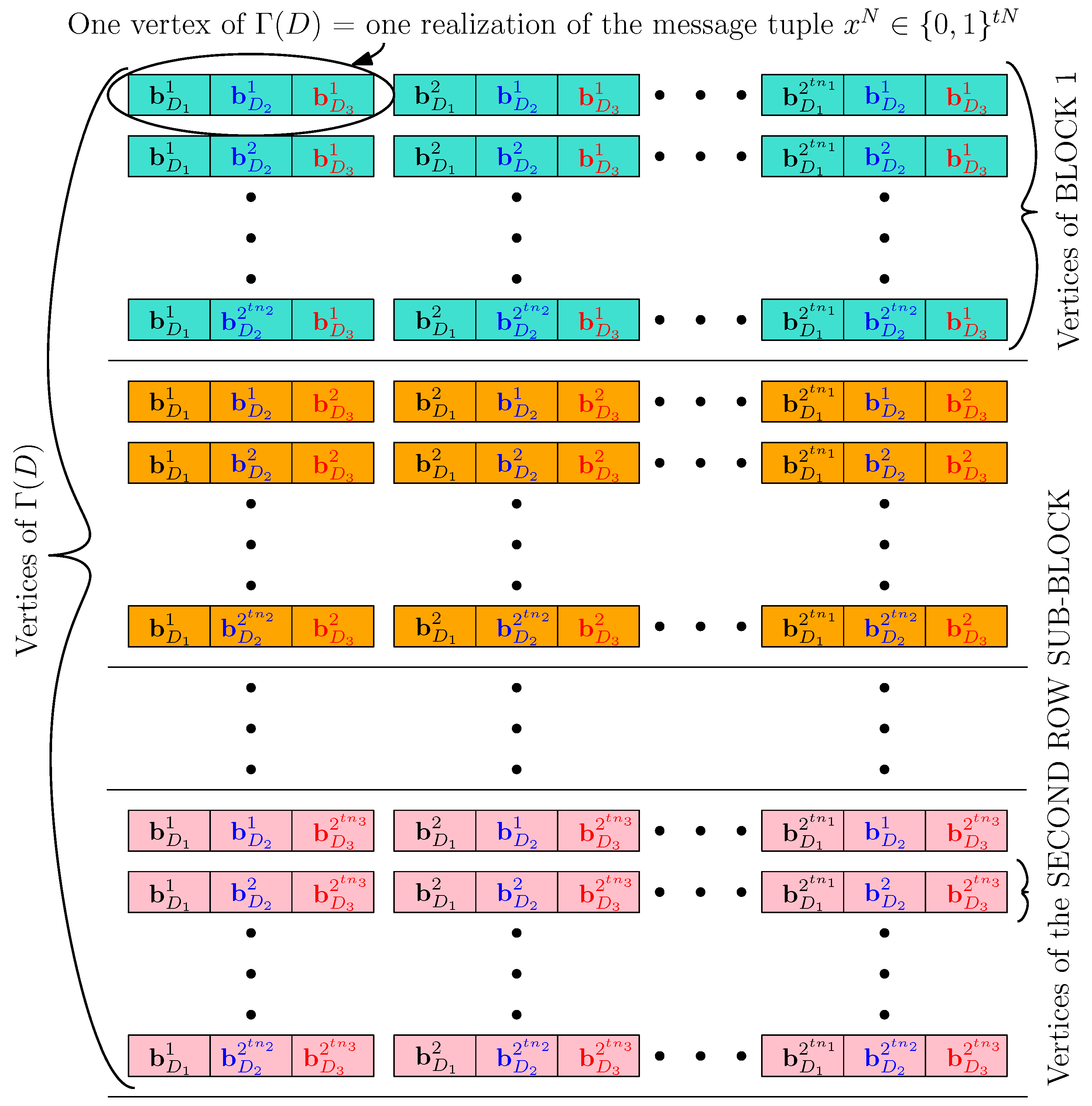
• Vertices labeled by all $({\mathbf{b}}_{D_1}^{i_1},{\mathbf{b}}_{D_2}^{i_2},{\mathbf{b}}_{D_3}^{i_3},\cdots ,{\mathbf{b}}_{D_{N^{\prime }}}^{i_{N^{\prime }}},{\mathbf{b}}_{D_{N^{\prime }+1}}^k)$, $i_j\in \{1,2,\cdots ,2^{t{n}_j}\}$, $j\in \{1,2,\cdots ,N^{\prime }\}$ and $k\in \{1,2,\cdots ,2^{t{n}_{N^{\prime }+1}}\}$, with the same ${\mathbf{b}}_{D_{N^{\prime }+1}}^k$ sub-label,
• any row sub-block consists of vertices labeled by all $({\mathbf{b}}_{D_1}^{i_1},{\mathbf{b}}_{D_2}^{i_2},{\mathbf{b}}_{D_3}^{i_3},\cdots ,{\mathbf{b}}_{D_{N^{\prime }}}^{i_{N^{\prime }}},{\mathbf{b}}_{D_{N^{\prime }+1}}^k)$, $i_j\in \{1,2,\cdots ,2^{t{n}_j}\}$, $j\in \{1,2,\cdots ,N^{\prime }\}$, with the same ${\mathbf{b}}_{D_2}^{i_2},{\mathbf{b}}_{D_3}^{i_3},\cdots ,{\mathbf{b}}_{D_{N^{\prime }}}^{i_{N^{\prime }}},{\mathbf{b}}_{D_{N^{\prime }+1}}^k$ sub-labels, and
• any $i_1$-th column sub-block consists of vertices labeled by all $({\mathbf{b}}_{D_1}^{i_1},{\mathbf{b}}_{D_2}^{i_2},{\mathbf{b}}_{D_3}^{i_3},\cdots ,{\mathbf{b}}_{D_{N^{\prime }}}^{i_{N^{\prime }}},{\mathbf{b}}_{D_{N^{\prime }+1}}^k)$, $i_j\in \{1,2,\cdots ,2^{t{n}_j}\}$, $j\in \{1,2,\cdots ,N^{\prime }\}$, with the same ${\mathbf{b}}_{D_1}^{i_1}$ and ${\mathbf{b}}_{D_{N^{\prime }+1}}^k$ sub-labels. Moreover, in contrast to SSUIC, there are multiple sub-labels other than ${\mathbf{b}}_{D_1}^{i_1}$ and ${\mathbf{b}}_{D_{N^{\prime }+1}}^k$ in MSUIC, so we arrange the vertices of any $i_1$-th column sub-block as dictated by Figure A2 in Appendix A. Clearly, a block has $2^{t{n}_1}$ column sub-blocks and $2^{t({\sum }_{i=2}^{N^{\prime }}{n}_i)}$ row sub-blocks.

Now, we illustrate the grouping of the vertices with an example. Assume that we have three senders $S_1$, $S_2$ and $S_3$ with ${\mathcal{M}}_1=\{x_1,x_4,x_5\}$, ${\mathcal{M}}_2=\{x_2,x_4,x_5\}$ and ${\mathcal{M}}_3=\{x_3,x_4,x_5\}$. We get $N^{\prime }=3$, and $V(D_4)=\{4,5\}$. For $x_i\in \{0,1\}$, $i\in \{1,2,3,4,5\}$, we arrange the vertices of the first block as shown in Figure 8.

Based on our classification of interactions (referring to Figure 3), ${\mathrm{H}}_1$ has no arc, and ${\mathrm{H}}_{16}$ has the following: Vertices 1 and 2, each has an out-degree of two, whereas the vertex 3 has zero out-degree. Now, considering the interactions between the sub-digraphs $D_1,D_2,\cdots ,D_{N^{\prime }},D_{N^{\prime }+1}$, the extensions of ${\mathrm{H}}_1$ and ${\mathrm{H}}_{16}$ to SMSUIC are straightforward (refer to Figure 9). We labeled them by ${\mathrm{H}}_1^{\prime }$ and ${\mathrm{H}}_{16}^{\prime }$, respectively, in SMSUIC. Now, we have the following proposition.

Proposition 4.

For any D having a fully-participated interaction between its sub-digraphs $D_1,D_2,\cdots ,D_{N^{\prime }},D_{N^{\prime }+1}$, if $f(D)\in \{{\mathrm{H}}_1^{\prime },{\mathrm{H}}_{16}^{\prime }\}$, then ${\beta }_t(D,G_o)={\sum }_{i=1}^{N^{\prime }+1}{\beta }_t(D_i)+ϵ/t$ for some $ϵ\in \{-N^{\prime },-N^{\prime }+1,\cdots ,0\}$.

Proof. 

Refer to Appendix G. □

Similar to the proof of Theorem 5, one can prove the following theorem using Proposition 4.

Theorem 9.

For any D having any interaction (i.e., either fully participated or partially participated) between its sub-digraphs $D_1,D_2,\cdots ,D_{N^{\prime }},D_{N^{\prime }+1}$, if $f(D)$ (i.e., $H^{\prime }$) has some arcs among its vertices $1,2,\cdots ,N^{\prime },N^{\prime }+1$ such that there is no out-going arc from $N^{\prime }+1$ to any other vertex, then ${\beta }_t(D,G_o)={\sum }_{i=1}^{N^{\prime }+1}{\beta }_t(D_i)+ϵ/t$ for some $ϵ\in \{-N^{\prime },-N^{\prime }+1,\cdots ,0\}$, and $\beta (D,G_o)={\sum }_{i=1}^{N^{\prime }+1}\beta (D_i)$.

Remark 7.

Extending the other cases of TSUIC to MSUIC is a laborious task as it involves a construction of multi-dimensional blocks and sub-blocks in a confusion graph.

7. Discussion

Consider any digraph D and its sub-digraphs $D_1$, $D_2$ and $D_3$. Let $d_D^{+}(u)$ be the out-degree of a vertex u of D. Now, we make the following two observations in TSUIC:

• The role of side-information of the vertices in $V(D_3)$ (vertices requesting the common messages) about the messages requested by vertices in $V(D_1)\cup V(D_2)$ (vertices requesting the private messages) in TSUIC: It is proved in SSUIC that, if the interaction between $D_1$, $D_2$ and $D_3$ is acyclic, i.e., $f(D)$ belongs to one of the digraphs in CASE I, then $\beta (D)=\beta (D_1)+\beta (D_2)+\beta (D_3)$ (by using Theorem 3). This means that the arcs contributing acyclic interactions between the sub-digraphs of D can be removed without affecting the optimal broadcast rate of D; in other words, those are non-critical arcs. In this paper, we have proved that this result is also true in TSUIC (by Theorem 5). Moreover, in TSUIC, we have proved that, for D, if the vertices in $V(D_3)$ have no side-information about the messages requested by vertices in $V(D_1)\cup V(D_2)$, i.e., $d_{f(D)}^{+}(3)=\varnothing$, then by Theorem 5, we have $\beta (D,G_o)=\beta (D_1)+\beta (D_2)+\beta (D_3)$ (behaves like having acyclic interactions between $D_1$, $D_2$ and $D_3$). Under this condition, any arc that is contributing any interaction between $D_1$, $D_2$ and $D_3$ is non-critical.
• Non-critical arcs in SSUIC are not necessarily non-critical in TSUIC: We illustrate this with an example. Consider the TSUIC problem stated in Example 1 (whose $f(D)={\mathrm{H}}_{33}$). In SSUIC, we know that the optimal broadcast rate $\beta (D)=2$. This problem has an arc $(3,1)$ that is non-critical in SSUIC (its removal does not change the optimal broadcast rate), but it is critical in TSUIC. This can be understood from the following: In SSUIC, we can remove the arc $(3,1)\in A(D)$, and still form a valid index code $\{x_1\oplus x_2,x_3\}$ that achieves $\beta (D)$. This infers that removing the arc $(3,1)$ does not affect the optimal broadcast rate in SSUIC. However, in TSUIC, if we remove the arc $(3,1)\in A(D)$, then the new problem, say $D^{\prime }$, has $\beta (D^{\prime },G_o)=3$ (applying Theorem 5), whereas we get a valid two-sender index code $\{x_1\oplus x_3,x_2\oplus x_3\}$ of codelength two if we consider $(3,1)\in A(D)$. Now, it is evident that there exist cases in TSUIC where some side-information (e.g., $(1,2)$ and $(2,1)$) cannot be exploited directly during encoding by senders because of the constraint due to the two senders. However, that side-information can be utilized during decoding process at receivers’ end due to the presence of other helping side-information (e.g., $(3,1)$). Thus, this helping side-information can be critical in TSUIC. This observation was also made by Sadeghi et al. [20] for MSUIC under a different performance metric (rate region with fixed capacity links).

8. Concluding Remarks and Open Problems

In this paper, we studied two-sender unicast-index-coding problems and established their structural characteristics. Noting that SSUIC is a well-studied problem (though for any arbitrary instance, it is still an open problem), there have been many important contributions made in the literature. In this paper, we solved TSUIC instances by expressing the optimal broadcast rates in terms of that of SSUIC. To this end, we introduced a two-sender graph coloring of confusion graphs in TSUIC, and propose a way of grouping the vertices of a confusion graph for analysis. Using these techniques, we derived optimal broadcast rates of TSUIC problems, both in the asymptotic and non-asymptotic regime, as a function of the optimal broadcast rates of their sub-problems. We have also presented a class of TSUIC instances where the interactions between the sub-problems of the problem are not critical. We illustrated that our proposed approach to TSUIC can be extended to some cases with multiple senders.

Some open problems for future works are the following:

• Study of the critical edges in the TSUIC problems: It is observed that the non-critical arcs in SSUIC can be critical arcs in TSUIC. This requires further study.
• Study of a general distributed index coding: As our study is a step towards understanding multi-sender index coding, it is left as a future work to extend the approaches implemented and the results obtained in this paper to more general setups.
• Finding the optimal broadcast rates of TSUIC problems with cyclic-partially-participated interactions: The analysis of D with partially-participated interactions between its sub-digraphs $D_1$, $D_2$ and $D_3$ is left as a future work.

References

- Birk, Y.; Kol, T. Informed-source coding-on-demand (ISCOD) over broadcast channels. Proc. IEEE INFOCOM 1998, 3, 1257–1264. [Google Scholar]
- Birk, Y.; Kol, T. Coding on demand by an informed source (ISCOD) for efficient broadcast of different supplemental data to caching clients. IEEE Trans. Inf. Theory 2006, 52, 2825–2830. [Google Scholar] [CrossRef]
- Bar-Yossef, Z.; Birk, Y.; Jayram, T.S.; Kol, T. Index Coding With Side Information. IEEE Trans. Inf. Theory 2011, 57, 1479–1494. [Google Scholar] [CrossRef]
- Blasiak, A.; Kleinberg, R.; Lubetzky, E. Broadcasting With Side Information: Bounding and Approximating the Broadcast Rate. IEEE Trans. Inf. Theory 2013, 59, 5811–5823. [Google Scholar] [CrossRef]
- Rouayheb, S.E.; Sprintson, A.; Georghiades, C. On the index coding problem and its relation to network coding and matroid theory. IEEE Trans. Inf. Theory 2010, 56, 3187–3195. [Google Scholar] [CrossRef]
- Maleki, H.; Cadambe, V.R.; Jafar, S.A. Index Coding—An Interference Alignment Perspective. IEEE Trans. Inf. Theory 2014, 60, 5402–5432. [Google Scholar] [CrossRef]
- Arbabjolfaei, F.; Bandemer, B.; Kim, Y.H.; Sasoglu, E.; Wang, L. On the capacity region for index coding. In Proceedings of the 2013 IEEE International Symposium on Information Theory (ISIT), Istanbul, Turkey, 7–12 July 2013; pp. 962–966. [Google Scholar]
- Arbabjolfaei, F.; Kim, Y.H. Structural properties of index coding capacity using fractional graph theory. In Proceedings of the 2015 IEEE International Symposium on Information Theory (ISIT), Hong Kong, China, 14–19 June 2015; pp. 1034–1038. [Google Scholar]
- Tahmasbi, M.; Shahrasbi, A.; Gohari, A. Critical Graphs in Index Coding. IEEE J. Sel. Areas Commun. 2015, 33, 225–235. [Google Scholar] [CrossRef]
- Shanmugam, K.; Dimakis, A.G.; Langberg, M. Local graph coloring and index coding. Proc. IEEE Int. Symp. Inf. Theory (ISIT) 2013, 1152–1156. [Google Scholar] [CrossRef]
- Ong, L. Optimal Finite-Length and Asymptotic Index Codes for Five or Fewer Receivers. IEEE Trans. Inf. Theory 2017, 63, 7116–7130. [Google Scholar] [CrossRef]
- Thapa, C.; Ong, L.; Johnson, S.J. Interlinked Cycles for Index Coding: Generalizing Cycles and Cliques. IEEE Trans. Inf. Theory 2017, 63, 3692–3711. [Google Scholar] [CrossRef]
- Thapa, C.; Ong, L.; Johnson, S.J. Corrections to Interlinked Cycles for Index Coding: Generalizing Cycles and Cliques. IEEE Trans. Inf. Theory 2018, 64, 6460. [Google Scholar] [CrossRef]
- Shanmugam, K.; Golrezaei, N.; Dimakis, A.G.; Molisch, A.F.; Caire, G. FemtoCaching: Wireless Content Delivery Through Distributed Caching Helpers. IEEE Trans. Inf. Theory 2013, 59, 8402–8413. [Google Scholar] [CrossRef]
- Rouayheb, S.E.; Sprintson, A.; Sadeghi, P. On coding for cooperative data exchange. Proc. IEEE Inf. Theory Workshop (ITW) 2010, 1–5. [Google Scholar] [CrossRef]
- Ong, L.; Ho, C.K.; Lim, F. The Single-Uniprior Index-Coding Problem: The Single-Sender Case and the Multi-Sender Extension. IEEE Trans. Inf. Theory 2016, 62, 3165–3182. [Google Scholar] [CrossRef]
- Thapa, C.; Ong, L.; Johnson, S.J. Graph-Theoretic Approaches to Two-Sender Index Coding. Proc. IEEE Globecom Workshops 2016, 1–6. [Google Scholar] [CrossRef]
- Chaudhry, M.A.R.; Asad, Z.; Sprintson, A.; Langberg, M. On the complementary Index Coding problem. Proc. IEEE Int. Symp. Inf. Theory (ISIT) 2011, 224–248. [Google Scholar] [CrossRef]
- Neely, M.J.; Tehrani, A.S.; Zhang, Z. Dynamic Index Coding for Wireless Broadcast Networks. IEEE Trans. Inf. Theory 2013, 59, 7525–7540. [Google Scholar] [CrossRef]
- Sadeghi, P.; Arbabjolfaei, F.; Kim, Y.H. Distributed Index Coding. Proc. IEEE Inf. Theory Workshop (ITW) 2016, 330–334. [Google Scholar] [CrossRef]
- Liu, Y.; Sadeghi, P.; Arbabjolfaei, F.; Kim, Y.H. On the Capacity for Distributed Index Coding. Proc. IEEE Int. Symp. Inf. Theory (ISIT) 2017, 3055–3059. [Google Scholar] [CrossRef]
- Li, M.; Ong, L.; Johnson, S.J. Improved Bounds for Multi-Sender Index Coding. Proc. IEEE Int. Symp. Inf. Theory (ISIT) 2017, 3060–3064. [Google Scholar] [CrossRef]
- Li, M.; Ong, L.; Johnson, S.J. Cooperative Multi-Sender Index Coding. IEEE Trans. Inf. Theory 2019, 65, 1725–1739. [Google Scholar] [CrossRef]
- Li, M.; Ong, L.; Johnson, S.J. Multi-Sender Index Coding for Collaborative Broadcasting: A Rank-Minimization Approach. IEEE Trans. on Comm. 2019, 67, 1452–1466. [Google Scholar] [CrossRef]
- Wan, K.; Tuninetti, D.; Ji, M.; Caire, G.; Piantanida, P. Fundamental Limits of Decentralized Data Shuffling. 2019. Available online: https://arxiv.org/pdf/1807.00056.pdf (accessed on 7 June 2019).
- Porter, A.; Wootters, M. Embedded Index Coding. 2019. Available online: https://arxiv.org/pdf/1904.02179.pdf (accessed on 7 June 2019).
- Arbabjolfaei, F. Index Coding: Fundamental Limits, Coding Schemes, and Structural Properties. Ph.D. Dissertation, University of California, San Diego, CA, USA, 2017. [Google Scholar]
- Alon, N.; Hassidim, A.; Lubetzky, E.; Stav, U.; Weinstein, A. Broadcasting with side information. In Proceedings of the 2008 49th Annual IEEE Symposium on Foundations of Computer Science, Philadelphia, PA, USA, 25–28 October 2008; pp. 823–832. [Google Scholar]
- Thapa, C.; Ong, L.; Johnson, S.J. Structural Characteristics of Two-Sender Index Coding. 2017. Available online: https://arxiv.org/pdf/1711.08150v1.pdf (accessed on 8 February 2019).
- Arunachala, C.; Rajan, B.S. Optimal Scalar Linear Index Codes for Three Classes of Two-Sender Unicast Index Coding Problem. 2018. Available online: https://arxiv.org/pdf/1804.03823.pdf (accessed on 18 January 2019).
- Arunachala, C.; Aggarwal, V.; Rajan, B.S. Optimal Linear Broadcast Rates of the Two-Sender Unicast Index Coding Problem with Fully-Participated Interactions. 2018. Available online: https://arxiv.org/pdf/1808.09775.pdf (accessed on 18 January 2019).
- Arunachala, C.; Aggarwal, V.; Rajan, B.S. On the Optimal Broadcast Rate of the Two-Sender Unicast Index Coding Problem with Fully-Participated Interactions. 2018. Available online: https://arxiv.org/pdf/1809.08116.pdf (accessed on 18 January 2019).
- Fekete, M. Uber die Verteilung der Wurzeln bei gewissen algebraischen Gleichungen mit ganzzahligen Koeffizienten. Math. Z. 1923, 17, 228–249. [Google Scholar] [CrossRef]
- Arbabjolfaei, F.; Kim, Y.H. On Critical Index Coding Problems. In Proceedings of the 2015 IEEE Information Theory Workshop - Fall (ITW), Jeju Island, Korea, 11–15 October 2015; pp. 9–13. [Google Scholar]
© 2019 by the authors. Licensee MDPI, Basel, Switzerland. This article is an open access article distributed under the terms and conditions of the Creative Commons Attribution (CC BY) license (http://creativecommons.org/licenses/by/4.0/).
Share and Cite
Thapa, C.; Ong, L.; Johnson, S.J.; Li, M. Structural Characteristics of Two-Sender Index Coding. Entropy 2019, 21, 615. https://doi.org/10.3390/e21060615
Thapa C, Ong L, Johnson SJ, Li M. Structural Characteristics of Two-Sender Index Coding. Entropy. 2019; 21(6):615. https://doi.org/10.3390/e21060615
Chicago/Turabian StyleThapa, Chandra, Lawrence Ong, Sarah J. Johnson, and Min Li. 2019. "Structural Characteristics of Two-Sender Index Coding" Entropy 21, no. 6: 615. https://doi.org/10.3390/e21060615
APA StyleThapa, C., Ong, L., Johnson, S. J., & Li, M. (2019). Structural Characteristics of Two-Sender Index Coding. Entropy, 21(6), 615. https://doi.org/10.3390/e21060615