
Design and Implementation of a New Local Alignment Algorithm for Multilayer Networks


Department of Medical and Surgical Sciences, Data Analytics Research Center, University Magna Græcia, 88100 Catanzaro, Italy
*
Author to whom correspondence should be addressed.
†
These authors contributed equally to this work.
Entropy 2022, 24(9), 1272; https://doi.org/10.3390/e24091272
Submission received: 9 August 2022
/
Revised: 6 September 2022
/
Accepted: 7 September 2022
/
Published: 9 September 2022
(This article belongs to the Special Issue Special Issue Dedicated to the 15th International Special Track on Biomedical and Bioinformatics Challenges for Computer Science)
Abstract
:Network alignment (NA) is a popular research field that aims to develop algorithms for comparing networks. Applications of network alignment span many fields, from biology to social network analysis. NA comes in two forms: global network alignment (GNA), which aims to find a global similarity, and LNA, which aims to find local regions of similarity. Recently, there has been an increasing interest in introducing complex network models such as multilayer networks. Multilayer networks are common in many application scenarios, such as modelling of relations among people in a social network or representing the interplay of different molecules in a cell or different cells in the brain. Consequently, the need to introduce algorithms for the comparison of such multilayer networks, i.e., local network alignment, arises. Existing algorithms for LNA do not perform well on multilayer networks since they cannot consider inter-layer edges. Thus, we propose local alignment of multilayer networks (MultiLoAl), a novel algorithm for the local alignment of multilayer networks. We define the local alignment of multilayer networks and propose a heuristic for solving it. We present an extensive assessment indicating the strength of the algorithm. Furthermore, we implemented a synthetic multilayer network generator to build the data for the algorithm’s evaluation.
1. Introduction
Network theory is one of the most important frameworks for a meaningful description and an efficient analysis of many complex systems [1,2,3]. Most popular analysis algorithms comprise the mining of a single network, e.g., using community detection algorithms [4]. In parallel, the comparison of networks has led to the introduction of many algorithms for comparing the structures on both a global and a local scale [5,6] that fall into the class of network alignment (NA) algorithms. The first class of algorithms, also known as global network alignment (GNA) algorithms, aims to find the overall similarity among networks. Differently, algorithms belonging to the second group are called local network alignment (LNA) algorithms and aim to find (relatively) small regions of similarity. The output of LNA algorithms is a set of matched regions (or subgraphs) among two graphs given as the input.
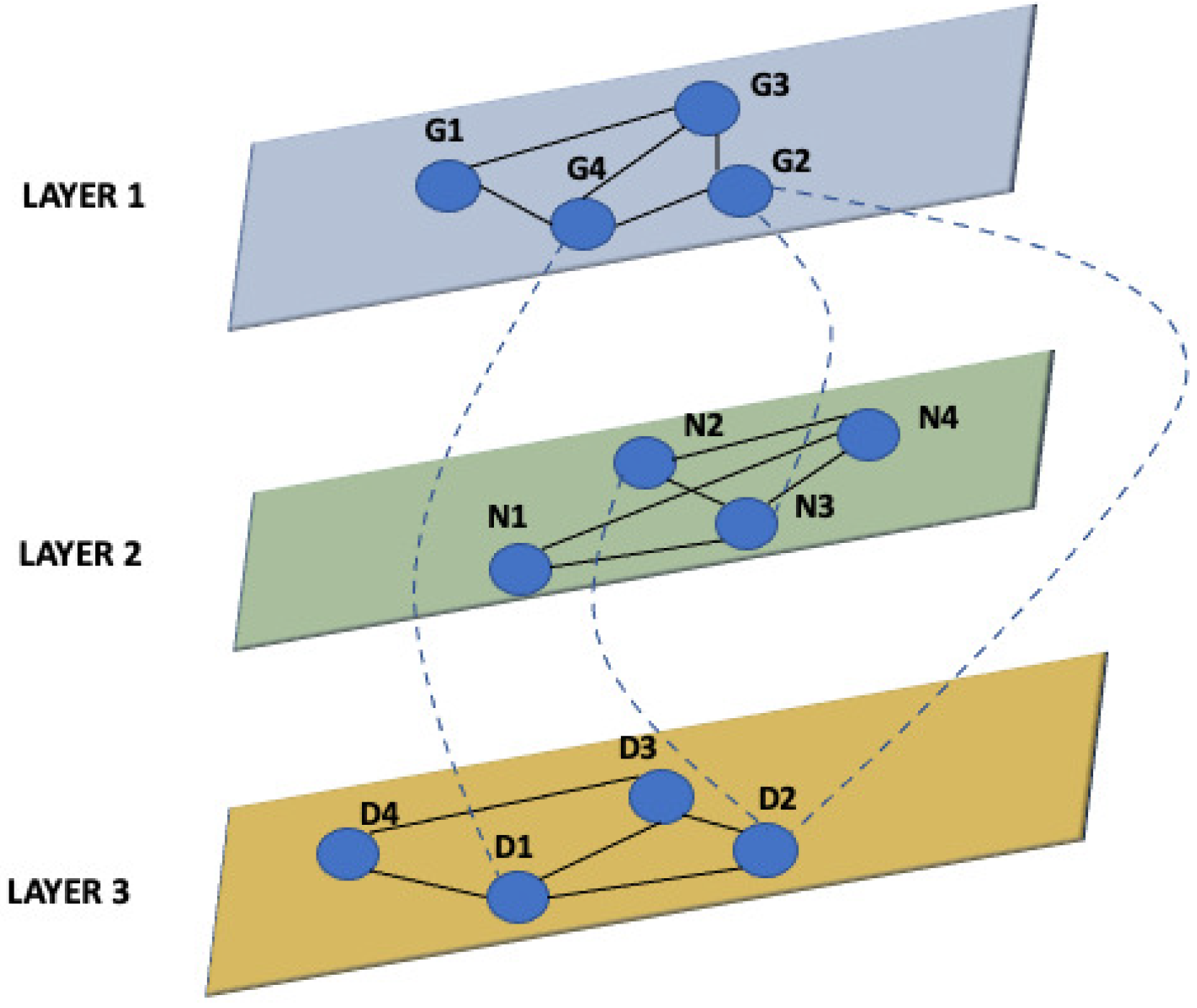
More recently, in many application fields, e.g., mobile and social networks and connectomics and metabolomics studies, the need for introducing models more complex than traditional networks arises [7,8]. In such contexts, nodes may have different classes of interactions among them, and such interactions may also be time-varying. In particular, networks representing multiple different associations among patients can be represented by a multilayer graph comprised of multiple interdependent graphs, where each graph represents an aspect or a set of similar interactions [9,10]. Figure 1 represents a simple multilayer graph with three layers. Each layer is a different graph G. Edges of a multilayer graph can be intra-layer, i.e., connecting nodes of the same layer, and inter-layer, i.e., connecting nodes of two different layers [11,12].
Formally, a multilayer network graph may be described as a tuple =, where is a set of layers and is a set of edges among layers. For each layer k, we have a graph (intra-layer edges), and for each pair of layers, k, h we have a set of edges , which is a set of layers connecting nodes of the layers v and k [13].
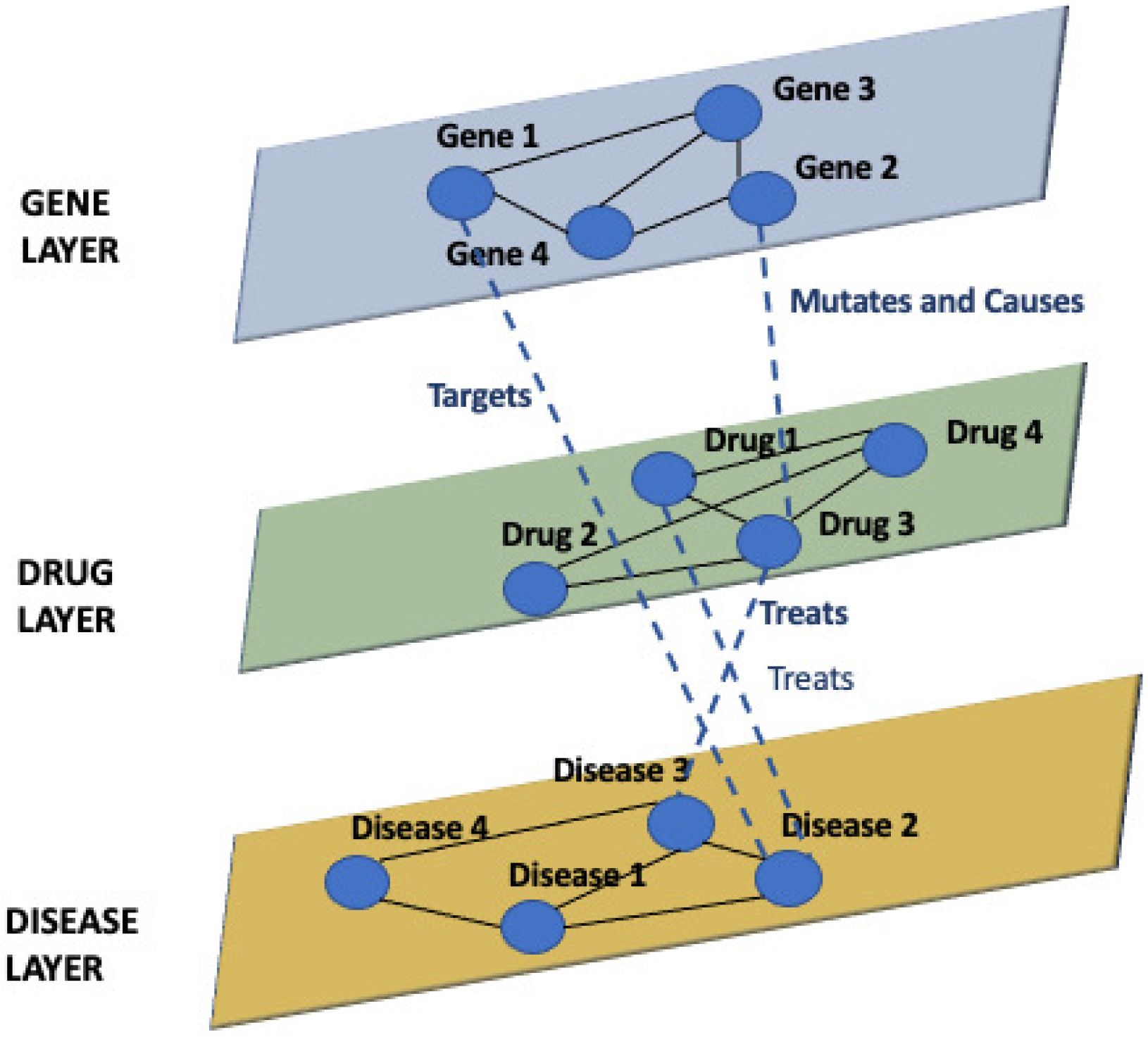
Examples of multilayer networks come from many different fields, from social network analysis to biological networks. For instance, Figure 2 represents an example of a biological multilayer network representing the interplay among diseases, genes, and drugs.
While many efforts have been made to address challenges related to the analysis of a single network, i.e., community detection in multilayer graphs, there is a need for the formalization and introduction of algorithms to compare multilayer networks. A simple strategy is an adaption or the simple use of existing algorithms for LNA. Unfortunately, this strategy is unsuitable, as previously demonstrated also in heterogeneous networks [14] because the the current algorithms are not able to manage the difference among layers.
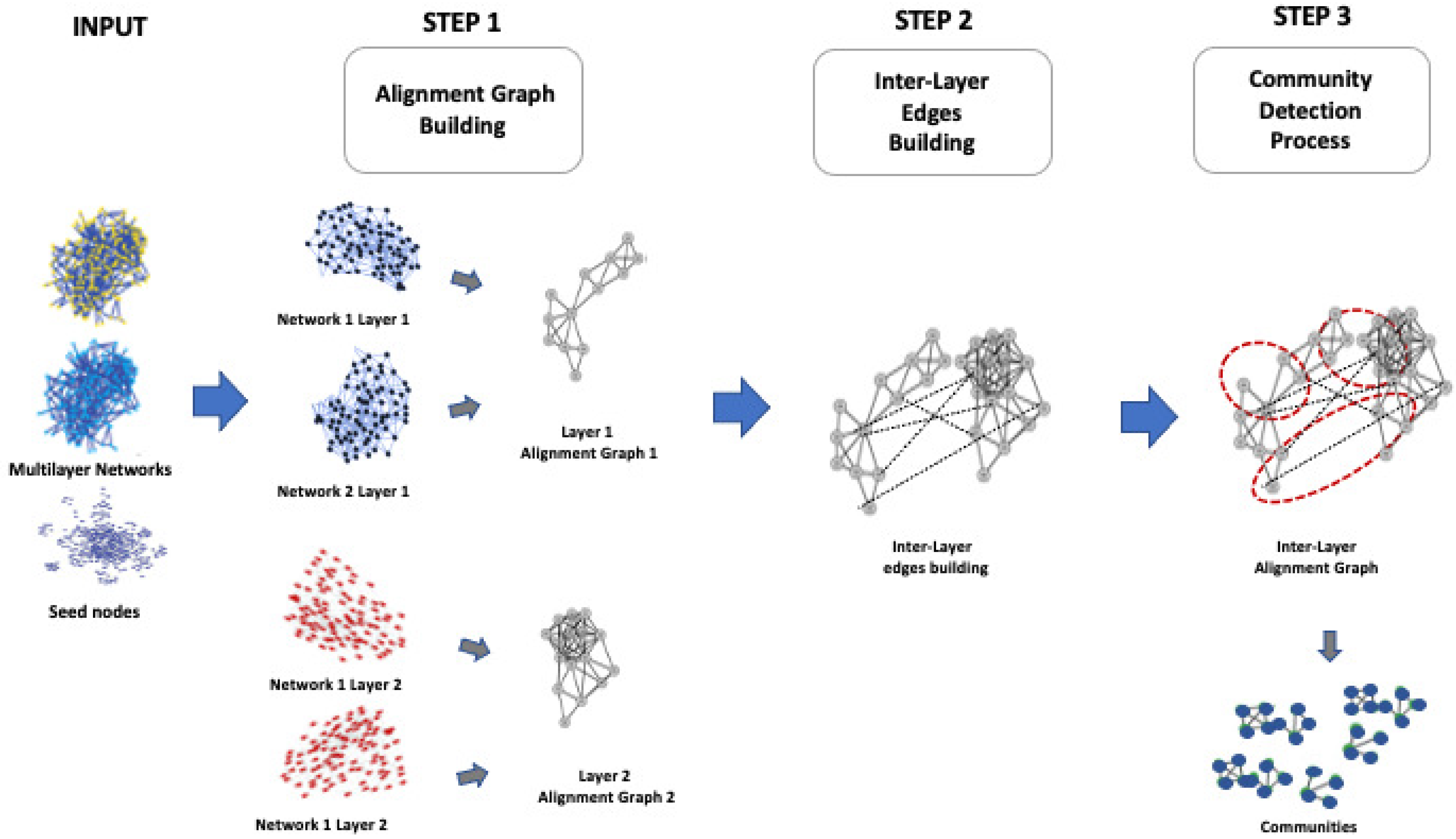
Thus, we propose local alignment of multilayer networks (MultiLoAl), a novel algorithm for the local alignment of multilayer networks. We define the local alignment of multilayer networks and propose a heuristic for solving it. MultiLoAl is based on an extension of the previous L-HetNetAligner [14], so it is based on the following steps, as depicted in Figure 3. Our algorithm receives two multilayer networks and a set of similarity relationships among nodes of the same layer in both networks used as the seed to build the alignment.
For instance, considering biological networks, similarity relations are represented by orthologs. The user may find these relations in databases of orthologs (e.g., OrthoMCL, etc.). It produces a set of multilayer graphs representing single local regions of the alignment.
The algorithm merges two input multilayer graphs into a single one, named the multilayer alignment graph, a multilayer graph with the same number of layers of the two inputs, and each layer represents an alignment graph of the same layer of the two input ones. For each node of a layer k, the alignment graph features pairs of nodes of the input ones. After building each alignment graph for each layer separately, we analyse the two input graphs to add inter-layer edges of the multilayer alignment graph. Finally, the algorithm uses a community detection algorithm suitable for multilayer graphs to detect communities representing local regions of similarity, i.e., a single region of the alignment. The result of our algorithm is a list of mappings among a subset of nodes of two networks, i.e., a set of mapped regions among input graphs.
We also realized a preliminary implementation of our algorithm by using the R programming language. We here refined such an implementation even in a high performance computing (HPC) fashion and provided deeper experimentation on a larger dataset. The main contributions of this paper are: (i) the implementation of a novel algorithm for the local alignment of multilayer networks, (ii) the definition of the local alignment of multilayer networks, (iii) the solution of a heuristic for solving it, and (iv) the implementation of a synthetic multilayer network generator to build the data for the algorithm evaluation.
2. Related Work
2.1. Alignment of Multilayer Networks
The alignment of networks aims to compare two or more networks [5], and existing algorithms may be categorised as local or global based on the approach, despite the existence of other classifications, i.e., algorithms for specific networks such as heterogeneous or temporal networks. Local network alignment (LNA) algorithms aim to find some similar (relatively) small subnetworks, while global network alignment (GNAs) algorithms search for the best superimposition of the whole compared networks. The literature contains many algorithms for other classes of networks (see, for instance, [5]). Unfortunately, the existing algorithms do not perform very well for multilayer networks [11,15].
2.2. Community Detection in Multilayer Networks
Community detection is one of the most popular research areas in various complex systems, such as biology, sociology, medicine, and transportation systems [16,17,18]. The reason is that the community structures, defined as groups of nodes that are more densely connected than the rest of the network, represent significant characteristics for understanding the functionalities and organisations of complex systems modelled as networks [16]. It is expected that the communities play significant roles in the structure–function relationship. For example, in biological networks such as protein–protein interaction (PPI) networks, the communities represent proteins involved in a similar function; in neuroscience, the communities detected in brain networks mean regions of interest (ROI) that are active during tasks; in social networks, communities can be groups of friends or colleagues; in the World Wild Web, the communities represent the web pages sharing the same topic [19]. Thus, the discovery of communities in these systems has become an interesting approach to figuring out how network structure relates to system behaviours.
Discovering a community structure in multilayer networks has became a hot research topic due to the inability of classical community detection methods to deal with the complexity of the multilayer model.
In fact, in multilayer networks, the communities represent groups of well-connected nodes in all layers. Thus, the detection algorithms should take into account the differences among layers. Unfortunately, traditional community detection methods are not able to deal with the complexity of the multilayer networks because (i) they do not enable analysing subsets of the layers and also (ii) they do not depict the diverse layers, and thus, they cannot distinguish between different types of multilayer communities [20]. To overcome these limitations, different community detection algorithms for multilayer networks have been recently proposed. For example, Infomap [21], a multilayer generalization of [22], is a method based on random walks. It considers that an entity randomly following the edges of a network would tend to become captured within communities due to the greater density of edges between nodes within the same community, moving less frequently from one community to another. This algorithm tries to identify a partition of vertices and levels that minimises the equation of the generalised map, which measures the length of the description of a random walk on the partition.
GenLouvain [23] is a multilayer generalisation of the iterative GenLouvain algorithm. This algorithm seeks a partition of the nodes and layers that maximises the multilayer modularity of the network. It searches the global information of the network, finding which are the edges of the network that contribute to the creation of the community structure; then, it applies a novel measure of edge centrality, to classify all the edges of the network concerning their proclivity to propagate information through the network itself.
ABACUS [24] is an algorithm that ensures the mining of multidimensional communities based on the extraction of frequent closed itemsets from monodimensional community memberships. At first, ABACUS considers each dimension independently, and it mines monodimensional communities. After that, it labels each node with a list of pair tags, i.e., the dimension and community the node belongs to in that dimension. Then, ABACUS considers each pair of tags as an item, and it applies a frequent-closed-itemset-mining algorithm. Finally, the multidimensional communities described by the itemsets consist of frequent closed itemsets.
Multilayer clique percolation [25] is a method that extends the popular clique percolation method for simple networks, where dense regions correspond to cliques and adjacency consists of having common nodes. The algorithm extends this step by searching cliques by encompassing multiple layers and reformulating adjacency so that both common nodes and common layers are expected. Multilayer clique percolation communities are combinations of adjacent cliques, so all the edges in these cliques can be considered part of the community.
Multidimensional label propagation (mdlp) [26] is an algorithm based on label propagation. At first, the algorithm assigns a different label to each node, and then, it weights the contribution of each neighbour based on their similarity with the nodes on the different layers. In particular, if two nodes are adjacent on all layers and have the same neighbours, they would have a higher probability of sharing the same label. Finally, the algorithm gives a score for each pair of nodes, referring to how likely a label should be extended from one to the other, bringing a common community.
3. MultiLoAl Algorithm
Initially, the algorithm inputs two multilayer networks and a set of similarities among node pairs of the same layer into the input networks. Then, it builds the alignment by performing two main steps: (i) construction of the multilayer alignment graph and (ii) mining of the multilayer alignment graph.
MultiLoAl analyses separately each corresponding pair of the corresponding layers of the input graphs. Each pair of a network of the same layer builds an alignment graph, as previously shown in L-HetNetAligner [14]. Then, it analyses the inter-layer edges of the input networks to add inter-layer edges to the multilayer alignment graph. Once the alignment graph is built, we use an algorithm for detecting communities in multilayer networks to uncover relevant modules. Figure 4 shows these steps.
MultiLoAl is a novel algorithm for the local alignment of multilayer networks. MultiLoAl builds the alignment on two main steps, as depicted in Figure 3:
- (i) Construction of the multilayer alignment graph;
- (ii) Analysis of the alignment graph.
Step (i) may be subdivided into two substeps: (i.a) adding nodes and intra-layer edges; (i.b) adding inter-layer edges.
Let us consider two multilayer input graphs and .
Node colours are used to distinguish different types of nodes belonging to two different types of layers. For simplicity, two multilayer input networks have the same number of nodes.
3.1. Step (1.a): Adding Nodes and Intra-Layer Edges to the Alignment Graph
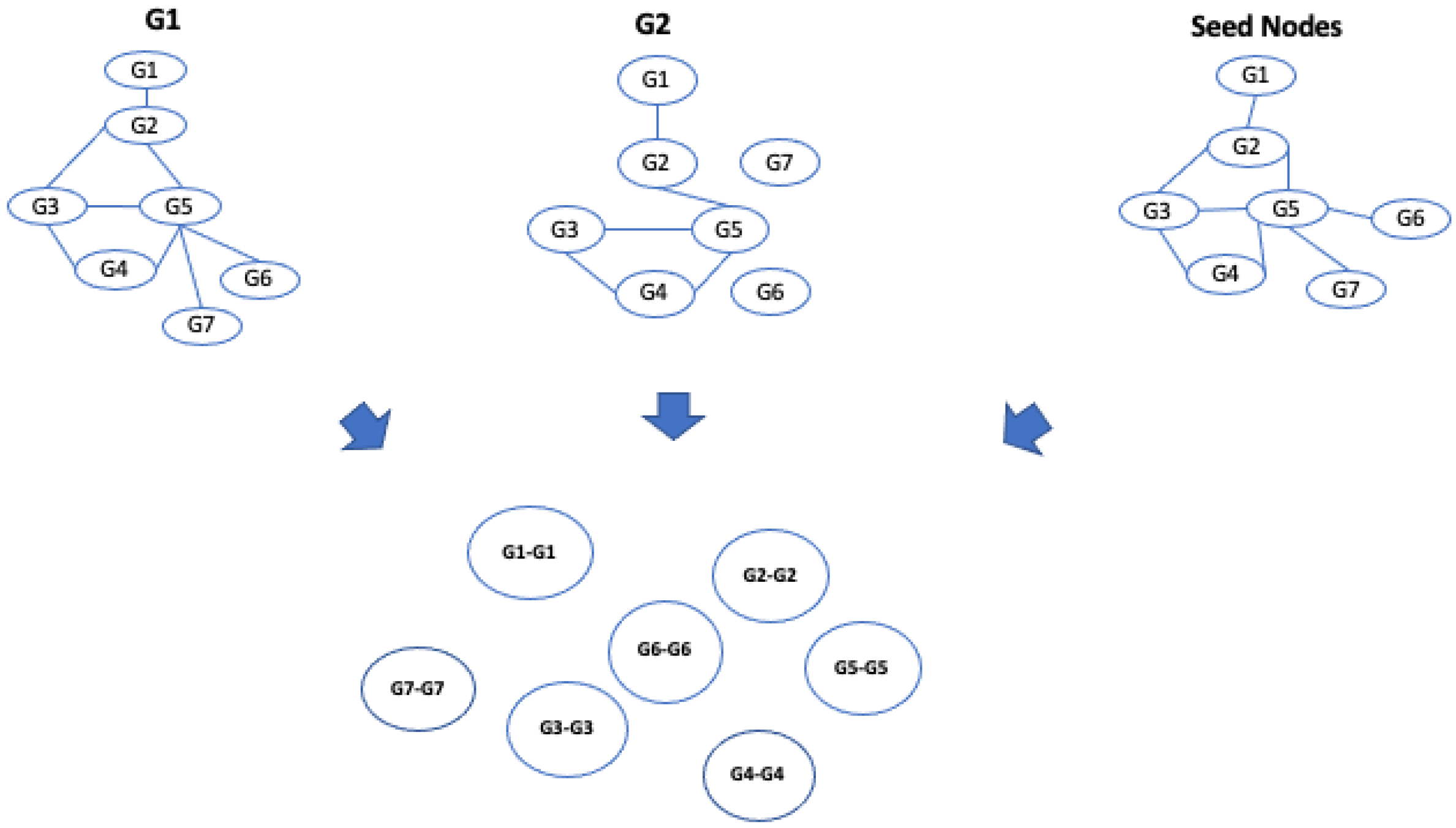
In the first step, the algorithm considers each pair of corresponding layers separately see Figure 5. For each layer, it builds an alignment graph following the approach proposed in L-HetNetAligner [14], adapted to the case of one-colour networks, as reported in Figure 6.
At this stage, the algorithm, starting from an initial list of seed nodes, builds the alignment graph by initially constructing two intermediate alignment graphs, which we call alignment graph layer 1 and alignment graph layer 2, for two networks belonging to layer 1 and two networks belonging to layer 2. Therefore, we define the alignment graph as a graph constructed by two initial input graphs and . Each node represents the matching of nodes of the input graphs, so . The selection of node pairs is guided by the input similarity relationships. Therefore, each node is matched with the most similar node of the other network through the use of the input similarity relationships, i.e., seed nodes; each node of the alignment graph represents a pair of similarities among nodes from the input networks; see Figure 7.
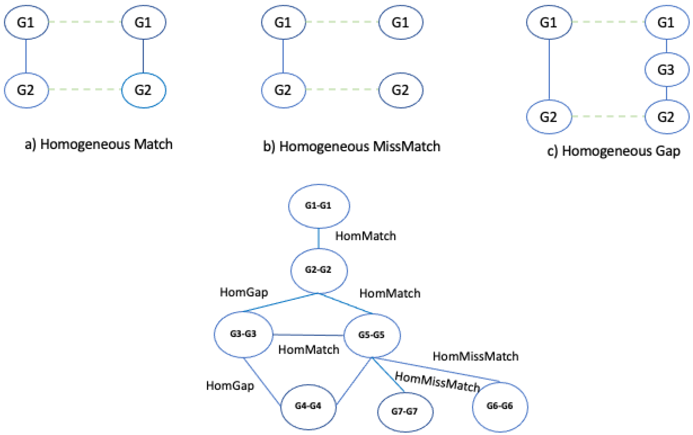
Once all nodes have been added to the graph, the algorithm builds the edges of the alignment graphs. For each pair of nodes, the algorithm examines the two input graphs, and it inserts and weights the edges considering three conditions: match, mismatch, and gap. Let us consider the nodes of the alignment graphs; in particular, let us consider the pair of nodes and in Figure 6. To determine the presence of an edge, we consider the edge network and network. If and contain these nodes and the nodes are adjacent, there is a match, which we call, for convenience, a homogeneous match, since the nodes of the two networks are of the same type (see Figure 8a).
Let us consider as the node distance, i.e., the length of the shortest connecting path threshold to discriminate between gaps and mismatches. If and contain these nodes and the nodes are adjacent only in a single network, there is a mismatch, which we call a homogeneous mismatch (Figure 8b).
If and contain these nodes, the nodes are adjacent only in a single network, and they are at a distance less than (gap threshold) in the other network, there is a gap, which we call a homogeneous gap (Figure 8c). After the edges of the alignment, graphs are added, and a weight is assigned to each edge by applying an ad hoc scoring function F and the gap threshold . The function assigns a high score to the matches than to the mismatches and gaps. The kind of scoring function has a large significance for the resulting alignment graph and on the alignment itself. The algorithm enables the user to choose other values to optimize the quality of the results. In this work, we set the weight assigned to each edge as follows: homogeneous match equal to 1, homogeneous mismatch equal to 0.5, homogeneous gap equal to 0.2.
3.2. Step (1.b): Adding Inter-Layer Edges
The algorithm adds the inter-layer edges among multilayer alignment graph layer 1 and alignment graph layer 2. For each pair of nodes in the multilayer alignment graphs, the algorithm examines the corresponding layers of the input graphs. Let us consider the pair of nodes and in Figure 8. To determine the presence of an edge, we consider the edge network and network. The initial graph contains both edges connecting their internal nodes, and if the nodes are adjacent, there is a match, which we call, for convenience, a heterogeneous match, since the nodes of the two networks are of different types; see Figure 9a.
Let us consider the pair of nodes and in Figure 8b. To determine the presence of an edge, we consider the edge network and network. contains the edge , while nodes and are disconnected in If the initial graph contains both edges connecting their internal nodes and the nodes are adjacent, there is a match, which we call, for convenience, a heterogeneous match, since the nodes of the two networks are of different types; see Figure 9a. Therefore, there is a heterogeneous mismatch (Figure 9b). Then, we set the weight assigned to each edge as follows: heterogeneous match equal to 0.9, heterogeneous mismatch equal to 0.4.
3.3. Step 2: Detection of Communities on the Alignment Graph
Finally, the final alignment graph is then mined to discover communities by applying a community detection algorithm by using existing algorithms for multilayer networks [27,28,29,30], see Figure 10. Our methodology presents a general design, so it is possible to mine the final alignment graph by applying a different mining method.
In the current version of MultiLoAl, we applied the Infomap algorithm to mine the communities on the alignment graph. However, the user can choose which community detection algorithm to select among Generalized Louvain, ABACUS, clique percolation, and mdlp. The output consists of a file that contains the extracted communities as a list of nodes, the weight of the edge, and the string in which it is reported if there is a homogeneous/heterogeneous match, homogeneous/mismatch, or homogeneous gap (see an example of the output at https://github.com/mmilano87/MultiLoAl (accessed on 12 August 2022)).
3.4. MultiLoAl vs. L-HetNetAligner
MultiLoAl, despite being based on the previous L-HetNetAligner, presents many different characteristics. First, the algorithms have different scopes: MultiLoAl is a local aligner of multilayer networks, while L-HetNetAligner works only on heterogeneous networks. In detail, by analysing the building of local alignment, MultiLoAl and L-HetNetAligner have two main general steps: (i) construction of the alignment graph; (ii) mining of the alignment graph. The building of the alignment graph is the first main difference among the two algorithms. In fact, MultiLoAl builds a multilayer alignment graph through two substeps: (i) by adding nodes and intra-layer edges, following the approach proposed in L-HetNetAligner adapted to the case of one-colour networks; (ii) by adding inter-layer edges. This last step represents the main novelty compared to L-HetNetAligner, because MultiLoAl analyses and adds the edges among different layers of input networks. Otherwise, L-HetNetAligner builds a heterogeneous alignment graph. Initially, L-HetNetAligner defines the nodes of the alignment graph as composite nodes representing pairs of nodes matched by the similarity considerations. The algorithm inserts and weights the edges in the alignment graph to the nodes for which the edge links have the same colour and according to their distance in the input network. Finally, once the alignment graph is built, both algorithms mine the alignment graph to discover modules that represent local alignment. MultiLoAl applies a community detection algorithm, Infomap, to mine the final alignment. The result consists of the extracted communities as a list of nodes, the weight of the edge, and the string in which it is reported if there is a homogeneous/heterogeneous match, homogeneous/mismatch, or homogeneous gap. Otherwise, L-HetNetAligner uses the Markov clustering (MCL) algorithm to cluster the graph. Each extracted module represents a single region of the alignment. The result of our algorithm is a list of mappings among a subset of nodes of two networks, i.e., a set of mapped regions among input graphs.
4. Results and Discussion
4.1. Evaluation of the Quality of the Alignment
The evaluation of the quality of the alignment of network is still a matter of debate for simple networks [5,31,32]. There exist many measures able to evaluate both the correctness of the alignment, as well as the quality of the obtained alignment [33]. On the other side, there is no gold standard to benchmark the alignment. Moreover, all the existing measures need to be extended in the multilayer case. Thus, we first introduce novel measures of correctness in the multilayer case (to the best of our knowledge, there are not any other available measures), then we perform an assessment of our methods. We first designed a proof of concept to show the ability of our algorithm to map correct nodes and edges by aligning a synthetic network with itself and with some randomised versions.
The correctness of an alignment is usually evaluated by means of the analysis of its topological quality, i.e., the ability to reconstruct the underlying true node mapping well (when such a mapping is known) and if it conserves many edges. For simple networks, (F-score node correctness) is a measure of node correctness, and it is a combination of two measures: and . is calculated as , and is defined as , where M is the set of node pairs that are mapped under the true node mapping and N is the set of node pairs that are aligned under an alignment f.
We here extended such a measure in the multilayer case. We first considered in a separate way each layer, and we calculated the for each layer . Then, we computed the multilayer as the average of all .
Similarly, the edge correctness in the simple case can be measured by considering NCV-G, which is a combination of two measures: high node coverage (NCV) and generalized (G). NCV is the percentage of nodes from and that are also in and , and G measures how well edges are conserved between and , where and are two graphs and and are subgraphs of and that are induced by the mapping.
We used NCV-G to measure the edge correctness of each layer , then we averaged the measures of such values for all the layers, and we obtained the multilayer NCV-G.
Finally, we should consider the edge correctness for the inter-layer edges. Without loss of information, we considered all the inter-layer edges as a whole, and we calculated the correctness of all the inter-layer edges as .
4.2. Proof of Concept
As a proof of principle, we present the use of the MultiLoAl dataset consisting of ten multilayer synthetic networks that we built with the graph generator, implemented ad hoc in the R code. An example of the multilayer network and R function are available on the web site of the project (https://github.com/mmilano87/MultiLoAl (accessed on 12 August 2022)).
All the multilayer networks have 30 nodes and 2 layers, whereas the edges are distributed as depicted in Table 1.
First, we aligned each network with respect to itself to show the ability to find known regions of similarity; second, we considered the alignment of the network with respect to an altered version of the network obtained by adding different levels of noise (5%, 10%, 15%, 20%, and 25%) by randomly removing edges from the network. The aim of the test was to demonstrate that the alignment algorithms are capable of producing high-quality alignments with an edge conservation of about 90%. Then, we implemented different versions of the MultiLoAl algorithm by varying the strategy applied to mine the community on the alignment graph. We executed the experiments on an Intel Core i5 Processor, 2.9 Ghz, with 4 Gbytes of main memory running the Ubuntu OS ver 18.04. MultiLoAl built 60 alignments, and it completed the whole process of alignment in ten seconds.
To measure the performance of the alignments built with different versions of MultiLoAl, we evaluated the quality of the results by considering the topological aspects of alignments and the number of communities found. At first, the results were evaluated by the topological quality.
We computed the NCV-G and F-NC measures for all alignment networks by considering the intra-layer and inter-layer edges. Table 2, Table 3, Table 4 and Table 5 report the results. Table 6, Table 7, Table 8 and Table 9 report the mean and standard deviation values of the NCV-G and F-NC measures for each synthetic network aligned with its noisy counterpart.
The results show that the quality of the alignment was greater when Infomap was applied to mine the community. Furthermore, increasing the noise level from 5% to 25% in the original networks caused NCV-G and F-NC to decrease.
5. Conclusions
Recently, the applications of multilayer networks in social network analysis, in finance, and in biology have been increasing. Multilayer networks can be seen as a set of networks (each network is a distinct layer) connected by inter-layer links. We here focused on the problem of comparing two multilayer networks, highlighting small local regions of similarity. Since existing algorithms for simple networks do not perform well on multilayer networks, we proposed Local Alignment of Multilayer Networks (MultiLoAl), a novel algorithm for the local alignment of multilayer networks. We proposed a heuristic for solving it. Furthermore, we performed an extensive evaluation to reveal the strength of the algorithm. Since we presented the use of MultiLoAl on multilayer synthetic networks, we plan to extend the application to real biological networks.
Author Contributions
Methodology, P.H.G. and M.M.; software, M.M.; data curation, M.M.; writing—original draft preparation, P.H.G. and M.C.; writing—review and editing, P.H.G., M.M. and M.C. funding acquisition, M.C. All authors have read and agreed to the published version of the manuscript.
Funding
This research received no external funding.
Institutional Review Board Statement
Not applicable.
Informed Consent Statement
Not applicable.
Data Availability Statement
https://github.com/mmilano87/MultiLoAl (accessed on 6 September 2022).
Acknowledgments
This work was partially funded by the following research project funded by PON “Ricerca e Innovazione” 2014-2020 (PON R&I) Ricercatori a Tempo Determinato di tipo A (RTDA) (DM 1062 del 10/08/2021) Asse IV—Istruzione e ricerca per il recupero—REACT-EU.
Conflicts of Interest
The authors declare no conflict of interest.
References
- Cannataro, M.; Guzzi, P.H.; Veltri, P. Protein-to-protein interactions: Technologies, databases, and algorithms. ACM Comput. Surv. (CSUR) 2010, 43, 1–36. [Google Scholar] [CrossRef]
- Barabasi, A.L.; Oltvai, Z.N. Network biology: Understanding the cell’s functional organization. Nat. Rev. Genet. 2004, 5, 101–113. [Google Scholar] [CrossRef] [PubMed]
- Gu, S.; Jiang, M.; Guzzi, P.H.; Milenković, T. Modeling multi-scale data via a network of networks. Bioinformatics 2022, 38, 2544–2553. [Google Scholar] [CrossRef] [PubMed]
- Fortunato, S. Community detection in graphs. Phys. Rep. Rev. Sec. Phys. Lett. 2010, 486, 75–174. [Google Scholar] [CrossRef]
- Guzzi, P.H.; Milenković, T. Survey of local and global biological network alignment: The need to reconcile the two sides of the same coin. Brief. Bioinform. 2018, 19, 472–481. [Google Scholar] [CrossRef]
- Hiram Guzzi, P.; Petrizzelli, F.; Mazza, T. Disease spreading modeling and analysis: A survey. Brief. Bioinform. 2022, 23, bbac230. [Google Scholar] [CrossRef]
- Boccaletti, S.; Bianconi, G.; Criado, R.; Del Genio, C.I.; Gómez-Gardenes, J.; Romance, M.; Sendina-Nadal, I.; Wang, Z.; Zanin, M. The structure and dynamics of multilayer networks. Phys. Rep. 2014, 544, 1–122. [Google Scholar] [CrossRef]
- Bianconi, G. Multilayer Networks: Structure and Function; Oxford University Press: Oxford, UK, 2018. [Google Scholar]
- Ortuso, F.; Mercatelli, D.; Guzzi, P.H.; Giorgi, F.M. Structural genetics of circulating variants affecting the SARS-CoV-2 spike/human ACE2 complex. J. Biomol. Struct. Dyn. 2021, 40, 1–11. [Google Scholar] [CrossRef]
- Gallo Cantafio, M.E.; Grillone, K.; Caracciolo, D.; Scionti, F.; Arbitrio, M.; Barbieri, V.; Pensabene, L.; Guzzi, P.H.; Di Martino, M.T. From single level analysis to multi-omics integrative approaches: A powerful strategy towards the precision oncology. High Throughput 2018, 7, 33. [Google Scholar] [CrossRef]
- Tagarelli, A.; Amelio, A.; Gullo, F. Ensemble-based community detection in multilayer networks. Data Min. Knowl. Discov. 2017, 31, 1506–1543. [Google Scholar] [CrossRef]
- Hammoud, Z.; Kramer, F. Multilayer networks: Aspects, implementations, and application in biomedicine. Big Data Anal. 2020, 5, 1–18. [Google Scholar] [CrossRef]
- Kivelä, M.; Arenas, A.; Barthelemy, M.; Gleeson, J.P.; Moreno, Y.; Porter, M.A. Multilayer networks. J. Complex Netw. 2014, 2, 203–271. [Google Scholar] [CrossRef]
- Milano, M.; Milenković, T.; Cannataro, M.; Guzzi, P.H. L-hetnetaligner: A novel algorithm for local alignment of heterogeneous biological networks. Sci. Rep. 2020, 10, 3901. [Google Scholar] [CrossRef]
- Ren, Y.; Sarkar, A.; Veltri, P.; Ay, A.; Dobra, A.; Kahveci, T. Pattern discovery in multilayer networks. IEEE ACM Trans. Comput. Biol. Bioinform. 2021, 19, 741–752. [Google Scholar] [CrossRef] [PubMed]
- Fortunato, S.; Hric, D. Community detection in networks: A user guide. Phys. Rep. 2016, 659, 1–44. [Google Scholar] [CrossRef]
- Lancichinetti, A.; Fortunato, S. Consensus clustering in complex networks. Sci. Rep. 2012, 2, 336. [Google Scholar] [CrossRef] [PubMed]
- Gligorijević, V.; Panagakis, Y.; Zafeiriou, S. Fusion and community detection in multi-layer graphs. In Proceedings of the 2016 23rd International Conference on Pattern Recognition (ICPR), Cancun, Mexico, 4–8 December 2016; pp. 1327–1332. [Google Scholar]
- Wang, Z.; Li, Z.; Yuan, G.; Sun, Y.; Rui, X.; Xiang, X. Tracking the evolution of overlapping communities in dynamic social networks. Knowl. Based Syst. 2018, 157, 81–97. [Google Scholar] [CrossRef]
- Magnani, M.; Hanteer, O.; Interdonato, R.; Rossi, L.; Tagarelli, A. Community detection in multiplex networks. ACM Comput. Surv. (CSUR) 2021, 54, 1–35. [Google Scholar] [CrossRef]
- De Domenico, M.; Lancichinetti, A.; Arenas, A.; Rosvall, M. Identifying modular flows on multilayer networks reveals highly overlapping organization in interconnected systems. Phys. Rev. X 2015, 5, 011027. [Google Scholar] [CrossRef]
- Rosvall, M.; Bergstrom, C.T. Maps of random walks on complex networks reveal community structure. Proc. Natl. Acad. Sci. USA 2008, 105, 1118–1123. [Google Scholar] [CrossRef] [Green Version]
- Jutla, I.S.; Jeub, L.G.; Mucha, P.J. A Generalized Louvain Method for Community Detection Implemented in MATLAB. 2011. Available online: http://netwiki.amath.unc.edu/GenLouvain (accessed on 7 July 2022).
- Berlingerio, M.; Pinelli, F.; Calabrese, F. ABACUS: Frequent pattern mining-based community discovery in multidimensional networks. Data Min. Knowl. Discov. 2013, 27, 294–320. [Google Scholar] [CrossRef]
- Afsarmanesh Tehrani, N.; Magnani, M. Partial and overlapping community detection in multiplex social networks. In Proceedings of the International Conference on Social Informatics; Springer: Cham, Switzerland, 2018; pp. 15–28. [Google Scholar]
- Boutemine, O.; Bouguessa, M. Mining community structures in multidimensional networks. ACM Trans. Knowl. Discov. Data (TKDD) 2017, 11, 1–36. [Google Scholar] [CrossRef]
- Kim, J.; Lee, J.G. Community detection in multi-layer graphs: A survey. ACM SIGMOD Rec. 2015, 44, 37–48. [Google Scholar] [CrossRef]
- Paul, S.; Chen, Y. Spectral and matrix factorization methods for consistent community detection in multi-layer networks. Ann. Stat. 2020, 48, 230–250. [Google Scholar] [CrossRef]
- Guzzi, P.H.; Salerno, E.; Tradigo, G.; Veltri, P. Extracting dense and connected communities in dual networks: An alignment based algorithm. IEEE Access 2020, 8, 162279–162289. [Google Scholar] [CrossRef]
- Huang, X.; Chen, D.; Ren, T.; Wang, D. A survey of community detection methods in multilayer networks. Data Min. Knowl. Discov. 2021, 35, 1–45. [Google Scholar] [CrossRef]
- Crawford, J.; Sun, Y.; Milenković, T. Fair evaluation of global network aligners. Algorithms Mol. Biol. 2015, 10, 1–17. [Google Scholar] [CrossRef]
- Hayes, W.B.; Mamano, N. SANA NetGO: A combinatorial approach to using Gene Ontology (GO) terms to score network alignments. Bioinformatics 2018, 34, 1345–1352. [Google Scholar] [CrossRef]
- Mina, M.; Guzzi, P.H. Improving the robustness of local network alignment: Design and extensive assessmentof a markov clustering-based approach. IEEE ACM Trans. Comput. Biol. Bioinform. 2014, 11, 561–572. [Google Scholar] [CrossRef]
Figure 1.
Example of a multilayer network. The figure represents a simple multilayer graph with three layers. Each layer is a different graph. Edges of a multilayer graph can be intra-layer, i.e., connecting nodes of the same layer, and inter-layer, i.e., connecting nodes of two different layers.
Figure 1.
Example of a multilayer network. The figure represents a simple multilayer graph with three layers. Each layer is a different graph. Edges of a multilayer graph can be intra-layer, i.e., connecting nodes of the same layer, and inter-layer, i.e., connecting nodes of two different layers.

Figure 2.
Example of a biological multilayer network.

Figure 3.
Local alignment of multilayer networks.

Figure 4.
Workflow of the proposed algorithm.

Figure 5.
The algorithm separates the input networks according to the layer type.

Figure 6.
Example of a multilayer network. The nodes represents a set of genes and a set of diseases that belong to the gene layer and the disease layer.
Figure 6.
Example of a multilayer network. The nodes represents a set of genes and a set of diseases that belong to the gene layer and the disease layer.

Figure 7.
Building of the alignment graph: node definition. The algorithm takes the two networks and a subset of node pairs matched according to a similarity function and starts to build the alignment graph. In this step, the algorithm defines the nodes of the alignment graph represented by the pair of matched nodes.

Figure 8.
Example of homogeneous match, homogeneous mismatch, and homogeneous gap and building of alignment graph.
Figure 8.
Example of homogeneous match, homogeneous mismatch, and homogeneous gap and building of alignment graph.

Figure 9.
Example of a homogeneous match, mismatch, and gap and building of inter-layer alignment graph.
Figure 9.
Example of a homogeneous match, mismatch, and gap and building of inter-layer alignment graph.

Figure 10.
Example of community detection extraction on inter-layer alignment graph.


Table 1.
Characteristics of the synthetic multilayer networks.
| Network | Layers | Nodes | Edges |
|---|---|---|---|
| N1 | 2 | 30 | 90 |
| N2 | 2 | 30 | 96 |
| N3 | 2 | 30 | 84 |
| N4 | 2 | 30 | 78 |
| N5 | 2 | 30 | 95 |
| N6 | 2 | 30 | 88 |
| N7 | 2 | 30 | 93 |
| N8 | 2 | 30 | 83 |
| N9 | 2 | 30 | 94 |
| N10 | 2 | 30 | 96 |
Table 2.
NCV-G values computed on intra-layer edges for all the alignments by applying Infomap, Generalized Louvain, ABACUS, clique percolation, and mdlp community detection algorithms.
Table 2.
NCV-G values computed on intra-layer edges for all the alignments by applying Infomap, Generalized Louvain, ABACUS, clique percolation, and mdlp community detection algorithms.
| Network | Noise | NCV-G with Infomap | NCV-G with Generalized Louvain | NCV-G with ABACUS | NCV-G with Clique Percolation | NCV-G with mdlp |
|---|---|---|---|---|---|---|
| N1 | 0 | 0.99 | 0.999 | 0.975 | 0.966 | 0.955 |
| 5 | 0.976 | 0.968 | 0.947 | 0.966 | 0.954 | |
| 10 | 0.96 | 0.92 | 0.925 | 0.942 | 0.95 | |
| 15 | 0.926 | 0.907 | 0.918 | 0.887 | 0.911 | |
| 20 | 0.914 | 0.891 | 0.903 | 0.887 | 0.906 | |
| 25 | 0.903 | 0.879 | 0.901 | 0.877 | 0.896 | |
| N2 | 0 | 0.995 | 0.996 | 0.951 | 0.966 | 0.976 |
| 5 | 0.964 | 0.992 | 0.843 | 0.912 | 0.829 | |
| 10 | 0.943 | 0.98 | 0.788 | 0.872 | 0.783 | |
| 15 | 0.941 | 0.953 | 0.773 | 0.862 | 0.708 | |
| 20 | 0.89 | 0.945 | 0.767 | 0.802 | 0.666 | |
| 25 | 0.881 | 0.894 | 0.766 | 0.792 | 0.615 | |
| N3 | 0 | 0.995 | 0.989 | 0.977 | 0.914 | 0.845 |
| 5 | 0.972 | 0.982 | 0.952 | 0.881 | 0.839 | |
| 10 | 0.961 | 0.956 | 0.883 | 0.815 | 0.836 | |
| 15 | 0.937 | 0.949 | 0.855 | 0.814 | 0.771 | |
| 20 | 0.933 | 0.923 | 0.801 | 0.73 | 0.754 | |
| 25 | 0.929 | 0.881 | 0.782 | 0.726 | 0.657 | |
| N4 | 0 | 0.979 | 0.999 | 0.976 | 0.854 | 0.809 |
| 5 | 0.979 | 0.97 | 0.959 | 0.849 | 0.744 | |
| 10 | 0.962 | 0.938 | 0.892 | 0.827 | 0.742 | |
| 15 | 0.915 | 0.914 | 0.844 | 0.82 | 0.698 | |
| 20 | 0.887 | 0.886 | 0.797 | 0.815 | 0.694 | |
| 25 | 0.881 | 0.885 | 0.788 | 0.721 | 0.691 | |
| N5 | 0 | 0.99 | 0.992 | 0.932 | 0.921 | 0.839 |
| 5 | 0.968 | 0.97 | 0.921 | 0.896 | 0.822 | |
| 10 | 0.957 | 0.963 | 0.881 | 0.89 | 0.756 | |
| 15 | 0.952 | 0.937 | 0.866 | 0.881 | 0.718 | |
| 20 | 0.935 | 0.92 | 0.845 | 0.817 | 0.717 | |
| 25 | 0.901 | 0.903 | 0.795 | 0.741 | 0.683 | |
| N6 | 0 | 0.994 | 0.966 | 0.969 | 0.872 | 0.968 |
| 5 | 0.968 | 0.943 | 0.968 | 0.81 | 0.913 | |
| 10 | 0.942 | 0.941 | 0.938 | 0.796 | 0.884 | |
| 15 | 0.932 | 0.936 | 0.836 | 0.765 | 0.834 | |
| 20 | 0.916 | 0.917 | 0.835 | 0.751 | 0.808 | |
| 25 | 0.891 | 0.909 | 0.76 | 0.741 | 0.665 | |
| N7 | 0 | 0.966 | 0.989 | 0.938 | 0.86 | 0.98 |
| 5 | 0.966 | 0.987 | 0.932 | 0.816 | 0.978 | |
| 10 | 0.956 | 0.959 | 0.855 | 0.807 | 0.9 | |
| 15 | 0.943 | 0.942 | 0.846 | 0.795 | 0.892 | |
| 20 | 0.941 | 0.898 | 0.841 | 0.765 | 0.87 | |
| 25 | 0.887 | 0.897 | 0.84 | 0.728 | 0.683 | |
| N8 | 0 | 0.997 | 0.96 | 0.969 | 0.954 | 0.969 |
| 5 | 0.98 | 0.957 | 0.955 | 0.839 | 0.812 | |
| 10 | 0.966 | 0.953 | 0.892 | 0.836 | 0.803 | |
| 15 | 0.956 | 0.951 | 0.837 | 0.825 | 0.791 | |
| 20 | 0.953 | 0.943 | 0.782 | 0.79 | 0.765 | |
| 25 | 0.922 | 0.895 | 0.772 | 0.726 | 0.764 | |
| N9 | 0 | 0.997 | 0.987 | 0.97 | 0.956 | 0.95 |
| 5 | 0.936 | 0.967 | 0.969 | 0.937 | 0.916 | |
| 10 | 0.923 | 0.967 | 0.95 | 0.93 | 0.786 | |
| 15 | 0.909 | 0.934 | 0.915 | 0.923 | 0.726 | |
| 20 | 0.882 | 0.928 | 0.8 | 0.874 | 0.635 | |
| 25 | 0.879 | 0.905 | 0.767 | 0.743 | 0.616 | |
| N10 | 0 | 0.991 | 0.986 | 0.948 | 0.972 | 0.839 |
| 5 | 0.982 | 0.958 | 0.872 | 0.959 | 0.825 | |
| 10 | 0.944 | 0.957 | 0.853 | 0.936 | 0.75 | |
| 15 | 0.938 | 0.943 | 0.839 | 0.871 | 0.689 | |
| 20 | 0.905 | 0.938 | 0.838 | 0.843 | 0.623 | |
| 25 | 0.904 | 0.911 | 0.811 | 0.757 | 0.603 |
Table 3.
NCV-G values computed on inter-layer edges for all the alignments by applying Infomap, Generalized Louvain, ABACUS, clique percolation, and mdlp community detection algorithms.
Table 3.
NCV-G values computed on inter-layer edges for all the alignments by applying Infomap, Generalized Louvain, ABACUS, clique percolation, and mdlp community detection algorithms.
| Network | Noise | NCV-G with Infomap | NCV-G with Generalized Louvain | NCV-G with ABACUS | NCV-G with Clique Percolation | NCV-G with mdlp |
|---|---|---|---|---|---|---|
| N1 | 0 | 0.76 | 0.76 | 0.745 | 0.711 | 0.576 |
| 5 | 0.727 | 0.727 | 0.691 | 0.706 | 0.571 | |
| 10 | 0.68 | 0.68 | 0.676 | 0.701 | 0.551 | |
| 15 | 0.641 | 0.641 | 0.664 | 0.678 | 0.537 | |
| 20 | 0.624 | 0.624 | 0.598 | 0.644 | 0.513 | |
| 25 | 0.617 | 0.617 | 0.567 | 0.599 | 0.506 | |
| N2 | 0 | 0.757 | 0.782 | 0.725 | 0.733 | 0.579 |
| 5 | 0.716 | 0.728 | 0.72 | 0.665 | 0.578 | |
| 10 | 0.709 | 0.711 | 0.714 | 0.662 | 0.555 | |
| 15 | 0.686 | 0.639 | 0.705 | 0.613 | 0.551 | |
| 20 | 0.672 | 0.63 | 0.701 | 0.598 | 0.505 | |
| 25 | 0.639 | 0.596 | 0.595 | 0.553 | 0.492 | |
| N3 | 0 | 0.735 | 0.771 | 0.727 | 0.707 | 0.6 |
| 5 | 0.734 | 0.693 | 0.725 | 0.705 | 0.592 | |
| 10 | 0.717 | 0.662 | 0.627 | 0.678 | 0.592 | |
| 15 | 0.676 | 0.656 | 0.61 | 0.638 | 0.532 | |
| 20 | 0.663 | 0.602 | 0.594 | 0.611 | 0.516 | |
| 25 | 0.618 | 0.589 | 0.578 | 0.595 | 0.504 | |
| N4 | 0 | 0.666 | 0.788 | 0.652 | 0.71 | 0.591 |
| 5 | 0.654 | 0.679 | 0.642 | 0.703 | 0.579 | |
| 10 | 0.645 | 0.588 | 0.632 | 0.683 | 0.528 | |
| 15 | 0.643 | 0.587 | 0.616 | 0.652 | 0.527 | |
| 20 | 0.638 | 0.586 | 0.6 | 0.583 | 0.509 | |
| 25 | 0.605 | 0.584 | 0.588 | 0.576 | 0.497 | |
| N5 | 0 | 0.791 | 0.781 | 0.713 | 0.711 | 0.591 |
| 5 | 0.759 | 0.778 | 0.703 | 0.711 | 0.587 | |
| 10 | 0.721 | 0.664 | 0.67 | 0.666 | 0.57 | |
| 15 | 0.721 | 0.607 | 0.643 | 0.626 | 0.529 | |
| 20 | 0.636 | 0.588 | 0.634 | 0.588 | 0.524 | |
| 25 | 0.636 | 0.585 | 0.573 | 0.564 | 0.518 | |
| N6 | 0 | 0.799 | 0.76 | 0.685 | 0.739 | 0.596 |
| 5 | 0.794 | 0.754 | 0.671 | 0.708 | 0.558 | |
| 10 | 0.79 | 0.729 | 0.605 | 0.698 | 0.538 | |
| 15 | 0.728 | 0.685 | 0.604 | 0.691 | 0.53 | |
| 20 | 0.719 | 0.651 | 0.571 | 0.552 | 0.518 | |
| 25 | 0.659 | 0.636 | 0.558 | 0.551 | 0.51 | |
| N7 | 0 | 0.754 | 0.73 | 0.703 | 0.629 | 0.59 |
| 5 | 0.728 | 0.697 | 0.675 | 0.613 | 0.571 | |
| 10 | 0.712 | 0.681 | 0.654 | 0.607 | 0.565 | |
| 15 | 0.706 | 0.651 | 0.631 | 0.57 | 0.56 | |
| 20 | 0.674 | 0.617 | 0.572 | 0.565 | 0.502 | |
| 25 | 0.639 | 0.592 | 0.563 | 0.56 | 0.499 | |
| N8 | 0 | 0.789 | 0.783 | 0.738 | 0.722 | 0.584 |
| 5 | 0.717 | 0.659 | 0.666 | 0.685 | 0.548 | |
| 10 | 0.684 | 0.623 | 0.589 | 0.639 | 0.54 | |
| 15 | 0.666 | 0.622 | 0.583 | 0.63 | 0.515 | |
| 20 | 0.618 | 0.621 | 0.576 | 0.627 | 0.509 | |
| 25 | 0.615 | 0.586 | 0.567 | 0.62 | 0.505 | |
| N9 | 0 | 0.767 | 0.77 | 0.727 | 0.728 | 0.588 |
| 5 | 0.75 | 0.749 | 0.722 | 0.674 | 0.584 | |
| 10 | 0.697 | 0.748 | 0.603 | 0.646 | 0.574 | |
| 15 | 0.67 | 0.729 | 0.575 | 0.637 | 0.547 | |
| 20 | 0.662 | 0.669 | 0.562 | 0.616 | 0.518 | |
| 25 | 0.609 | 0.584 | 0.553 | 0.564 | 0.504 | |
| N10 | 0 | 0.783 | 0.775 | 0.745 | 0.737 | 0.597 |
| 5 | 0.744 | 0.761 | 0.678 | 0.725 | 0.586 | |
| 10 | 0.721 | 0.741 | 0.666 | 0.654 | 0.574 | |
| 15 | 0.703 | 0.666 | 0.664 | 0.653 | 0.541 | |
| 20 | 0.649 | 0.654 | 0.607 | 0.59 | 0.528 | |
| 25 | 0.643 | 0.648 | 0.598 | 0.57 | 0.508 |
Table 4.
F-NC values computed on intra-layer edges for all the alignments by applying Infomap, Generalized Louvain, ABACUS, clique percolation, and mdlp community detection algorithms.
Table 4.
F-NC values computed on intra-layer edges for all the alignments by applying Infomap, Generalized Louvain, ABACUS, clique percolation, and mdlp community detection algorithms.
| Network | Noise | F-NC with Infomap | F-NC with Generalized Louvain | F-NC with ABACUS | F-NC with Clique Percolation | F-NC with mdlp |
|---|---|---|---|---|---|---|
| N1 | 0 | 0.626 | 0.575 | 0.591 | 0.53 | 0.568 |
| 5 | 0.62 | 0.566 | 0.573 | 0.518 | 0.54 | |
| 10 | 0.608 | 0.556 | 0.558 | 0.511 | 0.528 | |
| 15 | 0.601 | 0.549 | 0.528 | 0.502 | 0.512 | |
| 20 | 0.599 | 0.528 | 0.505 | 0.501 | 0.504 | |
| 25 | 0.568 | 0.524 | 0.501 | 0.492 | 0.479 | |
| N2 | 0 | 0.643 | 0.605 | 0.571 | 0.555 | 0.552 |
| 5 | 0.643 | 0.603 | 0.566 | 0.55 | 0.506 | |
| 10 | 0.619 | 0.598 | 0.565 | 0.537 | 0.5 | |
| 15 | 0.61 | 0.596 | 0.542 | 0.528 | 0.483 | |
| 20 | 0.605 | 0.581 | 0.534 | 0.521 | 0.461 | |
| 25 | 0.587 | 0.523 | 0.53 | 0.51 | 0.452 | |
| N3 | 0 | 0.648 | 0.609 | 0.58 | 0.576 | 0.546 |
| 5 | 0.609 | 0.603 | 0.542 | 0.556 | 0.532 | |
| 10 | 0.599 | 0.598 | 0.541 | 0.553 | 0.532 | |
| 15 | 0.58 | 0.592 | 0.516 | 0.516 | 0.502 | |
| 20 | 0.578 | 0.59 | 0.516 | 0.516 | 0.473 | |
| 25 | 0.577 | 0.57 | 0.507 | 0.507 | 0.47 | |
| N4 | 0 | 0.628 | 0.608 | 0.584 | 0.576 | 0.552 |
| 5 | 0.626 | 0.592 | 0.567 | 0.573 | 0.54 | |
| 10 | 0.612 | 0.581 | 0.558 | 0.553 | 0.537 | |
| 15 | 0.57 | 0.557 | 0.557 | 0.544 | 0.528 | |
| 20 | 0.565 | 0.53 | 0.497 | 0.536 | 0.509 | |
| 25 | 0.559 | 0.517 | 0.495 | 0.521 | 0.473 | |
| N5 | 0 | 0.649 | 0.601 | 0.6 | 0.559 | 0.531 |
| 5 | 0.648 | 0.557 | 0.592 | 0.526 | 0.516 | |
| 10 | 0.637 | 0.555 | 0.578 | 0.483 | 0.511 | |
| 15 | 0.635 | 0.542 | 0.55 | 0.482 | 0.485 | |
| 20 | 0.626 | 0.541 | 0.547 | 0.472 | 0.474 | |
| 25 | 0.618 | 0.539 | 0.503 | 0.471 | 0.451 | |
| N6 | 0 | 0.636 | 0.578 | 0.587 | 0.566 | 0.525 |
| 5 | 0.633 | 0.577 | 0.572 | 0.56 | 0.516 | |
| 10 | 0.587 | 0.546 | 0.539 | 0.553 | 0.499 | |
| 15 | 0.58 | 0.532 | 0.527 | 0.545 | 0.482 | |
| 20 | 0.568 | 0.528 | 0.519 | 0.507 | 0.468 | |
| 25 | 0.561 | 0.514 | 0.49 | 0.483 | 0.467 | |
| N7 | 0 | 0.642 | 0.608 | 0.572 | 0.567 | 0.542 |
| 5 | 0.634 | 0.606 | 0.568 | 0.547 | 0.537 | |
| 10 | 0.597 | 0.573 | 0.543 | 0.502 | 0.536 | |
| 15 | 0.597 | 0.568 | 0.521 | 0.491 | 0.507 | |
| 20 | 0.565 | 0.511 | 0.505 | 0.49 | 0.501 | |
| 25 | 0.554 | 0.51 | 0.499 | 0.488 | 0.47 | |
| N8 | 0 | 0.625 | 0.59 | 0.585 | 0.571 | 0.551 |
| 5 | 0.601 | 0.555 | 0.565 | 0.504 | 0.537 | |
| 10 | 0.591 | 0.554 | 0.547 | 0.492 | 0.515 | |
| 15 | 0.583 | 0.541 | 0.545 | 0.486 | 0.514 | |
| 20 | 0.552 | 0.522 | 0.54 | 0.483 | 0.508 | |
| 25 | 0.551 | 0.52 | 0.533 | 0.472 | 0.466 | |
| N9 | 0 | 0.639 | 0.605 | 0.594 | 0.568 | 0.563 |
| 5 | 0.632 | 0.596 | 0.583 | 0.56 | 0.523 | |
| 10 | 0.607 | 0.574 | 0.579 | 0.554 | 0.513 | |
| 15 | 0.582 | 0.561 | 0.555 | 0.53 | 0.498 | |
| 20 | 0.575 | 0.542 | 0.54 | 0.512 | 0.456 | |
| 25 | 0.574 | 0.523 | 0.507 | 0.509 | 0.455 | |
| N10 | 0 | 0.641 | 0.597 | 0.581 | 0.57 | 0.505 |
| 5 | 0.614 | 0.579 | 0.554 | 0.52 | 0.492 | |
| 10 | 0.603 | 0.558 | 0.522 | 0.51 | 0.478 | |
| 15 | 0.557 | 0.526 | 0.519 | 0.494 | 0.47 | |
| 20 | 0.552 | 0.526 | 0.509 | 0.491 | 0.469 | |
| 25 | 0.551 | 0.513 | 0.491 | 0.484 | 0.461 |
Table 5.
F-NC values computed on inter-layer edges for all the alignments by applying Infomap, Generalized Louvain, ABACUS, clique percolation, and mdlp community detection algorithms.
Table 5.
F-NC values computed on inter-layer edges for all the alignments by applying Infomap, Generalized Louvain, ABACUS, clique percolation, and mdlp community detection algorithms.
| Network | Noise | F-NC with Infomap | F-NC with Generalized Louvain | F-NC with ABACUS | F-NC with Clique Percolation | F-NC with mdlp |
|---|---|---|---|---|---|---|
| N1 | 0 | 0.566 | 0.577 | 0.555 | 0.548 | 0.465 |
| 5 | 0.55 | 0.573 | 0.509 | 0.543 | 0.462 | |
| 10 | 0.545 | 0.539 | 0.496 | 0.533 | 0.46 | |
| 15 | 0.533 | 0.519 | 0.474 | 0.493 | 0.448 | |
| 20 | 0.531 | 0.516 | 0.472 | 0.473 | 0.441 | |
| 25 | 0.501 | 0.482 | 0.467 | 0.471 | 0.429 | |
| N2 | 0 | 0.591 | 0.566 | 0.548 | 0.539 | 0.485 |
| 5 | 0.568 | 0.545 | 0.548 | 0.498 | 0.478 | |
| 10 | 0.522 | 0.532 | 0.524 | 0.497 | 0.461 | |
| 15 | 0.512 | 0.517 | 0.504 | 0.477 | 0.452 | |
| 20 | 0.506 | 0.506 | 0.483 | 0.471 | 0.402 | |
| 25 | 0.503 | 0.499 | 0.471 | 0.455 | 0.401 | |
| N3 | 0 | 0.561 | 0.576 | 0.553 | 0.548 | 0.476 |
| 5 | 0.559 | 0.548 | 0.511 | 0.548 | 0.469 | |
| 10 | 0.553 | 0.547 | 0.505 | 0.511 | 0.447 | |
| 15 | 0.55 | 0.543 | 0.489 | 0.496 | 0.446 | |
| 20 | 0.531 | 0.496 | 0.483 | 0.467 | 0.425 | |
| 25 | 0.502 | 0.485 | 0.483 | 0.463 | 0.425 | |
| N4 | 0 | 0.596 | 0.577 | 0.534 | 0.543 | 0.467 |
| 5 | 0.561 | 0.574 | 0.529 | 0.516 | 0.465 | |
| 10 | 0.547 | 0.568 | 0.513 | 0.51 | 0.446 | |
| 15 | 0.53 | 0.531 | 0.511 | 0.49 | 0.442 | |
| 20 | 0.528 | 0.505 | 0.505 | 0.482 | 0.44 | |
| 25 | 0.512 | 0.482 | 0.462 | 0.458 | 0.402 | |
| N5 | 0 | 0.588 | 0.569 | 0.538 | 0.52 | 0.47 |
| 5 | 0.585 | 0.524 | 0.527 | 0.52 | 0.45 | |
| 10 | 0.585 | 0.5 | 0.524 | 0.512 | 0.412 | |
| 15 | 0.565 | 0.486 | 0.499 | 0.472 | 0.403 | |
| 20 | 0.516 | 0.485 | 0.492 | 0.463 | 0.403 | |
| 25 | 0.507 | 0.485 | 0.475 | 0.455 | 0.401 | |
| N6 | 0 | 0.578 | 0.564 | 0.543 | 0.539 | 0.481 |
| 5 | 0.565 | 0.554 | 0.541 | 0.533 | 0.471 | |
| 10 | 0.554 | 0.542 | 0.536 | 0.498 | 0.466 | |
| 15 | 0.552 | 0.539 | 0.525 | 0.493 | 0.457 | |
| 20 | 0.536 | 0.533 | 0.513 | 0.492 | 0.412 | |
| 25 | 0.518 | 0.518 | 0.496 | 0.481 | 0.41 | |
| N7 | 0 | 0.587 | 0.525 | 0.545 | 0.548 | 0.488 |
| 5 | 0.573 | 0.513 | 0.502 | 0.522 | 0.479 | |
| 10 | 0.555 | 0.51 | 0.495 | 0.52 | 0.476 | |
| 15 | 0.529 | 0.507 | 0.483 | 0.514 | 0.465 | |
| 20 | 0.529 | 0.496 | 0.48 | 0.491 | 0.462 | |
| 25 | 0.508 | 0.482 | 0.471 | 0.454 | 0.419 | |
| N8 | 0 | 0.598 | 0.579 | 0.553 | 0.52 | 0.486 |
| 5 | 0.59 | 0.563 | 0.532 | 0.511 | 0.473 | |
| 10 | 0.578 | 0.563 | 0.517 | 0.494 | 0.439 | |
| 15 | 0.56 | 0.561 | 0.512 | 0.481 | 0.437 | |
| 20 | 0.535 | 0.549 | 0.478 | 0.48 | 0.413 | |
| 25 | 0.524 | 0.48 | 0.461 | 0.478 | 0.41 | |
| N9 | 0 | 0.597 | 0.56 | 0.538 | 0.55 | 0.479 |
| 5 | 0.59 | 0.54 | 0.522 | 0.537 | 0.472 | |
| 10 | 0.578 | 0.538 | 0.497 | 0.497 | 0.469 | |
| 15 | 0.545 | 0.535 | 0.496 | 0.476 | 0.461 | |
| 20 | 0.54 | 0.509 | 0.479 | 0.466 | 0.456 | |
| 25 | 0.515 | 0.501 | 0.464 | 0.465 | 0.41 | |
| N10 | 0 | 0.598 | 0.541 | 0.539 | 0.532 | 0.475 |
| 5 | 0.566 | 0.54 | 0.505 | 0.531 | 0.473 | |
| 10 | 0.561 | 0.527 | 0.471 | 0.53 | 0.471 | |
| 15 | 0.56 | 0.509 | 0.47 | 0.475 | 0.448 | |
| 20 | 0.55 | 0.495 | 0.468 | 0.456 | 0.418 | |
| 25 | 0.546 | 0.487 | 0.466 | 0.451 | 0.414 |
Table 6.
NCV-G mean and standard deviation values computed on intra-layer edges for all the alignments by applying Infomap, Generalized Louvain, ABACUS, clique percolation, and mdlp community detection algorithms.
Table 6.
NCV-G mean and standard deviation values computed on intra-layer edges for all the alignments by applying Infomap, Generalized Louvain, ABACUS, clique percolation, and mdlp community detection algorithms.
| Network | Measure | NCV-G with Infomap | NCV-G with Generalized Louvain | NCV-G with ABACUS | NCV-G with Clique Percolation | NCV-G with mdlp |
|---|---|---|---|---|---|---|
| N1 | mean | 0.945 | 0.927 | 0.928 | 0.921 | 0.929 |
| sd | 0.035 | 0.047 | 0.028 | 0.042 | 0.027 | |
| N2 | mean | 0.936 | 0.960 | 0.815 | 0.868 | 0.763 |
| sd | 0.044 | 0.038 | 0.073 | 0.066 | 0.130 | |
| N3 | mean | 0.955 | 0.947 | 0.875 | 0.813 | 0.784 |
| sd | 0.026 | 0.040 | 0.079 | 0.077 | 0.073 | |
| N4 | mean | 0.934 | 0.932 | 0.876 | 0.814 | 0.730 |
| sd | 0.045 | 0.046 | 0.080 | 0.048 | 0.046 | |
| N5 | mean | 0.951 | 0.948 | 0.873 | 0.858 | 0.756 |
| sd | 0.030 | 0.033 | 0.051 | 0.067 | 0.063 | |
| N6 | mean | 0.941 | 0.935 | 0.884 | 0.789 | 0.845 |
| sd | 0.037 | 0.020 | 0.086 | 0.048 | 0.105 | |
| N7 | mean | 0.943 | 0.945 | 0.875 | 0.795 | 0.884 |
| sd | 0.030 | 0.041 | 0.047 | 0.045 | 0.109 | |
| N8 | mean | 0.962 | 0.943 | 0.868 | 0.828 | 0.817 |
| sd | 0.026 | 0.024 | 0.085 | 0.075 | 0.077 | |
| N9 | mean | 0.921 | 0.948 | 0.895 | 0.894 | 0.772 |
| sd | 0.043 | 0.031 | 0.089 | 0.079 | 0.140 | |
| N10 | mean | 0.944 | 0.949 | 0.860 | 0.890 | 0.722 |
| sd | 0.037 | 0.025 | 0.047 | 0.082 | 0.100 |
Table 7.
NCV-G mean and standard deviation values computed on inter-layer edges for all the alignments by applying Infomap, Generalized Louvain, ABACUS, clique percolation, and mdlp community detection algorithms.
Table 7.
NCV-G mean and standard deviation values computed on inter-layer edges for all the alignments by applying Infomap, Generalized Louvain, ABACUS, clique percolation, and mdlp community detection algorithms.
| Network | Measure | NCV-G with Infomap | NCV-G with Generalized Louvain | NCV-G with ABACUS | NCV-G with Clique Percolation | NCV-G with mdlp |
|---|---|---|---|---|---|---|
| N1 | mean | 0.675 | 0.675 | 0.657 | 0.673 | 0.542 |
| sd | 0.058 | 0.058 | 0.065 | 0.044 | 0.029 | |
| N2 | mean | 0.697 | 0.681 | 0.693 | 0.637 | 0.543 |
| sd | 0.041 | 0.071 | 0.049 | 0.063 | 0.037 | |
| N3 | mean | 0.691 | 0.662 | 0.644 | 0.656 | 0.556 |
| sd | 0.046 | 0.066 | 0.066 | 0.048 | 0.043 | |
| N4 | mean | 0.642 | 0.635 | 0.622 | 0.651 | 0.539 |
| sd | 0.021 | 0.083 | 0.025 | 0.059 | 0.038 | |
| N5 | mean | 0.711 | 0.667 | 0.656 | 0.644 | 0.553 |
| sd | 0.063 | 0.092 | 0.051 | 0.062 | 0.033 | |
| N6 | mean | 0.748 | 0.703 | 0.616 | 0.657 | 0.542 |
| sd | 0.056 | 0.053 | 0.052 | 0.083 | 0.031 | |
| N7 | mean | 0.702 | 0.661 | 0.633 | 0.591 | 0.548 |
| sd | 0.041 | 0.051 | 0.056 | 0.029 | 0.038 | |
| N8 | mean | 0.682 | 0.649 | 0.620 | 0.654 | 0.534 |
| sd | 0.066 | 0.070 | 0.068 | 0.041 | 0.030 | |
| N9 | mean | 0.693 | 0.708 | 0.624 | 0.644 | 0.553 |
| sd | 0.059 | 0.070 | 0.080 | 0.055 | 0.035 | |
| N10 | mean | 0.707 | 0.708 | 0.660 | 0.655 | 0.556 |
| sd | 0.054 | 0.058 | 0.053 | 0.068 | 0.035 |
Table 8.
F-NC mean and standard deviation values computed on intra-layer edges for all the alignments by applying Infomap, Generalized Louvain, ABACUS, clique percolation, and mdlp community detection algorithms.
Table 8.
F-NC mean and standard deviation values computed on intra-layer edges for all the alignments by applying Infomap, Generalized Louvain, ABACUS, clique percolation, and mdlp community detection algorithms.
| Network | Measure | F-NC with Infomap | F-NC with Generalized Louvain | F-NC with ABACUS | F-NC with Clique Percolation | F-NC with mdlp |
|---|---|---|---|---|---|---|
| N1 | mean | 0.604 | 0.550 | 0.543 | 0.509 | 0.522 |
| sd | 0.020 | 0.020 | 0.037 | 0.014 | 0.031 | |
| N2 | mean | 0.618 | 0.584 | 0.551 | 0.534 | 0.492 |
| sd | 0.022 | 0.031 | 0.018 | 0.017 | 0.036 | |
| N3 | mean | 0.599 | 0.594 | 0.534 | 0.537 | 0.509 |
| sd | 0.028 | 0.014 | 0.027 | 0.028 | 0.033 | |
| N4 | mean | 0.593 | 0.564 | 0.543 | 0.551 | 0.523 |
| sd | 0.032 | 0.036 | 0.038 | 0.021 | 0.028 | |
| N5 | mean | 0.636 | 0.556 | 0.562 | 0.499 | 0.495 |
| sd | 0.012 | 0.023 | 0.036 | 0.036 | 0.030 | |
| N6 | mean | 0.594 | 0.546 | 0.539 | 0.536 | 0.493 |
| sd | 0.033 | 0.027 | 0.036 | 0.033 | 0.025 | |
| N7 | mean | 0.598 | 0.563 | 0.535 | 0.514 | 0.516 |
| sd | 0.035 | 0.044 | 0.031 | 0.034 | 0.028 | |
| N8 | mean | 0.584 | 0.547 | 0.553 | 0.501 | 0.515 |
| sd | 0.029 | 0.026 | 0.019 | 0.036 | 0.029 | |
| N9 | mean | 0.602 | 0.567 | 0.560 | 0.539 | 0.501 |
| sd | 0.029 | 0.031 | 0.032 | 0.025 | 0.042 | |
| N10 | mean | 0.586 | 0.550 | 0.529 | 0.512 | 0.479 |
| sd | 0.038 | 0.034 | 0.033 | 0.032 | 0.016 |
Table 9.
F-NC mean and standard deviation values computed on inter-layer edges for all the alignments by applying Infomap, Generalized Louvain, ABACUS, clique percolation, and mdlp community detection algorithms.
Table 9.
F-NC mean and standard deviation values computed on inter-layer edges for all the alignments by applying Infomap, Generalized Louvain, ABACUS, clique percolation, and mdlp community detection algorithms.
| Network | Measure | F-NC with Infomap | F-NC with Generalized Louvain | F-NC with ABACUS | F-NC with Clique Percolation | F-NC with mdlp |
|---|---|---|---|---|---|---|
| N1 | mean | 0.538 | 0.534 | 0.496 | 0.510 | 0.451 |
| sd | 0.022 | 0.036 | 0.033 | 0.035 | 0.014 | |
| N2 | mean | 0.534 | 0.528 | 0.513 | 0.490 | 0.447 |
| sd | 0.037 | 0.025 | 0.033 | 0.029 | 0.037 | |
| N3 | mean | 0.543 | 0.533 | 0.504 | 0.506 | 0.448 |
| sd | 0.023 | 0.035 | 0.027 | 0.037 | 0.021 | |
| N4 | mean | 0.546 | 0.540 | 0.509 | 0.500 | 0.444 |
| sd | 0.030 | 0.040 | 0.026 | 0.030 | 0.023 | |
| N5 | mean | 0.543 | 0.533 | 0.504 | 0.506 | 0.448 |
| sd | 0.023 | 0.035 | 0.027 | 0.037 | 0.021 | |
| N6 | mean | 0.558 | 0.508 | 0.509 | 0.490 | 0.423 |
| sd | 0.037 | 0.033 | 0.024 | 0.030 | 0.029 | |
| N7 | mean | 0.547 | 0.506 | 0.496 | 0.508 | 0.465 |
| sd | 0.030 | 0.015 | 0.026 | 0.032 | 0.024 | |
| N8 | mean | 0.564 | 0.549 | 0.509 | 0.494 | 0.443 |
| sd | 0.030 | 0.035 | 0.034 | 0.018 | 0.031 | |
| N9 | mean | 0.561 | 0.531 | 0.499 | 0.499 | 0.458 |
| sd | 0.032 | 0.022 | 0.027 | 0.037 | 0.025 | |
| N10 | mean | 0.564 | 0.517 | 0.487 | 0.496 | 0.450 |
| sd | 0.018 | 0.023 | 0.030 | 0.039 | 0.028 |
Publisher’s Note: MDPI stays neutral with regard to jurisdictional claims in published maps and institutional affiliations. |
© 2022 by the authors. Licensee MDPI, Basel, Switzerland. This article is an open access article distributed under the terms and conditions of the Creative Commons Attribution (CC BY) license (https://creativecommons.org/licenses/by/4.0/).
Share and Cite
MDPI and ACS Style
Milano, M.; Guzzi, P.H.; Cannataro, M. Design and Implementation of a New Local Alignment Algorithm for Multilayer Networks. Entropy 2022, 24, 1272. https://doi.org/10.3390/e24091272
AMA Style
Milano M, Guzzi PH, Cannataro M. Design and Implementation of a New Local Alignment Algorithm for Multilayer Networks. Entropy. 2022; 24(9):1272. https://doi.org/10.3390/e24091272
Chicago/Turabian StyleMilano, Marianna, Pietro Hiram Guzzi, and Mario Cannataro. 2022. "Design and Implementation of a New Local Alignment Algorithm for Multilayer Networks" Entropy 24, no. 9: 1272. https://doi.org/10.3390/e24091272
Note that from the first issue of 2016, this journal uses article numbers instead of page numbers. See further details here.