Molecular Dynamics on Wood-Derived Lignans Analyzed by Intermolecular Network Theory


Abstract
: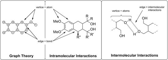
1. Introduction
2. Results and Discussion
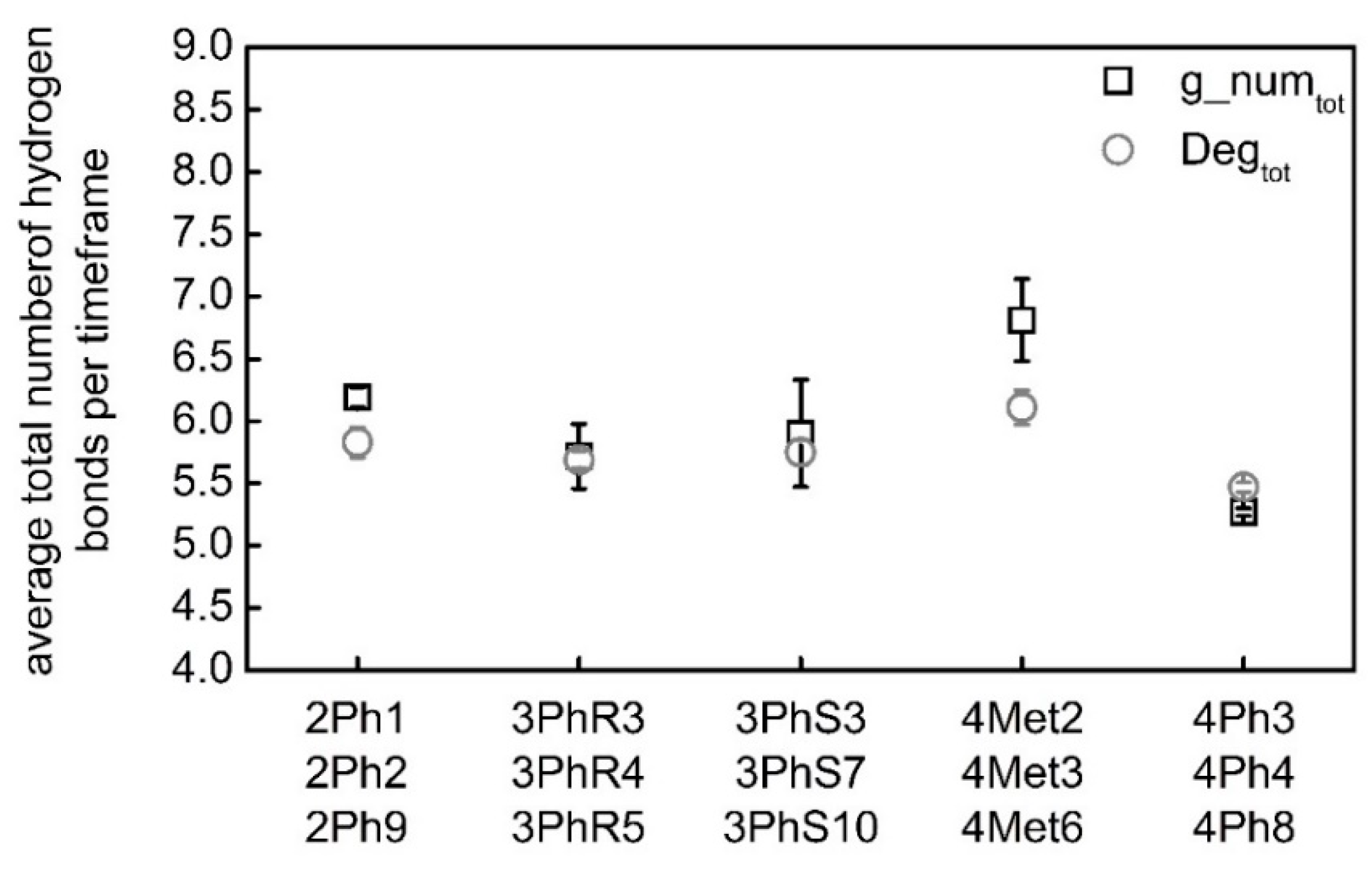
2.1. Hydration
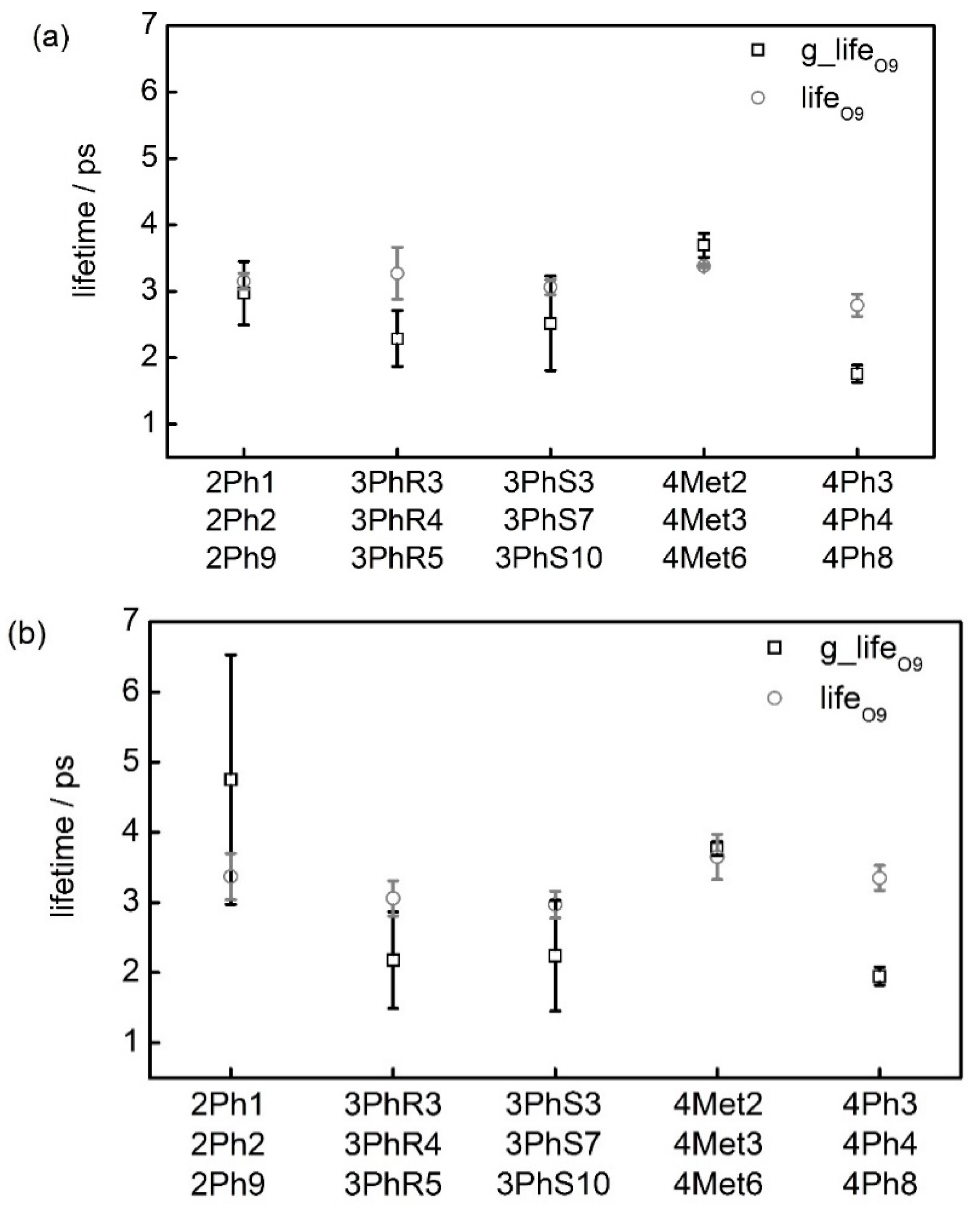
2.2. Lifetime of Hydrogen Bonds
2.3. Distance Distributions
3. Materials and Methods
Data Format and Working Procedure
4. Conclusions
Author Contributions
Funding
Acknowledgments
Conflicts of Interest
References
- Van der Spoel, D.; van Maaren, P.J.; Larsson, P.; Tîmneanu, N. Thermodynamics of hydrogen bonding in hydrophilic and hydrophobic media. J. Phys. Chem. B 2006, 110, 4393–4398. [Google Scholar] [CrossRef] [PubMed]
- Smith, P.E.; Pettitt, B.M. Modeling solvent in biomolecular systems. J. Phys. Chem. 1994, 98, 9700–9711. [Google Scholar] [CrossRef]
- Jorgensen, W.L.; Tirado-Rives, J. Potential energy functions for atomic-level simulations of water and organic and biomolecular systems. Proc. Natl. Acad. Sci. USA 2005, 102, 6665–6670. [Google Scholar] [CrossRef] [PubMed] [Green Version]
- Kuo, J.L.; Coe, J.V.; Singer, S.J.; Band, Y.B.; Ojamäe, L. On the use of graph invariants for efficiently generating hydrogen bond topologies and predicting physical properties of water clusters and ice. J. Chem. Phys. 2001, 114, 2527–2540. [Google Scholar] [CrossRef]
- Mooney, B.L.; Corrales, L.R.; Clark, A.E. MoleculaRnetworks: An integrated graph theoretic and data mining tool to explore solvent organization in molecular simulation. J. Comput. Chem. 2012, 33, 853–860. [Google Scholar] [CrossRef] [PubMed]
- Mooney, B.L.; Corrales, L.R.; Clark, A.E. Novel analysis of cation solvation using a graph theoretic approach. J. Phys. Chem. B 2012, 116, 4263–4275. [Google Scholar] [CrossRef] [PubMed]
- Hudelson, M.; Mooney, B.L.; Clark, A.E. Determining polyhedral arrangements of atoms using PageRank. J. Math. Chem. 2012, 50, 2342–2350. [Google Scholar] [CrossRef]
- Ozkanlar, A.; Clark, A.E. ChemNetworks: A complex network analysis tool for chemical systems. J. Comput. Chem. 2013, 35, 495–505. [Google Scholar] [CrossRef] [PubMed]
- Seebach, D.; Beck, A.K.; Schiess, M.; Widler, L.; Wonnacott, A. Some recent advances in the use of titanium reagents for organic synthesis. Pure Appl. Chem. 1983, 55, 1807–1822. [Google Scholar] [CrossRef]
- Sandberg, T.; Brusentsev, Y.; Eklund, P.; Hotokka, M. Structural analysis of sterically hindered 1,4-diols from the naturally occurring lignan hydroxymatairesinol a quantum chemical study. Int. J. Quantum Chem. 2011, 111, 4309–4317. [Google Scholar] [CrossRef]
- Sandberg, T.; Eklund, P.; Hotokka, M. Conformational solvation studies of LIGNOLs with molecular dynamics and conductor-like screening model. Int. J. Mol. Sci. 2012, 13, 9845–9863. [Google Scholar] [CrossRef] [PubMed]
- Brusentsev, Y.; Sandberg, T.; Hotokka, M.; Sjöholm, R.; Eklund, P. Synthesis and structural analysis of sterically hindered chiral 1,4-diol ligands derived from the lignan hydroxymatairesinol. Tetrahedron Lett. 2013, 54, 1112–1115. [Google Scholar] [CrossRef]
- Sandberg, T.; Eklund, P. The effect of density functional dispersion correction (DFT-D3) on lignans. Comput. Theor. Chem. 2015, 1067, 60–63. [Google Scholar] [CrossRef]
- Sandberg, T. Computational Chemistry Studies of Wood-Derived Lignans; Åbo Akademi University: Turku, Finland, 2013. [Google Scholar]
- Bekker, H.; Berendsen, H.J.C.; Dijkstra, E.J.; Achterop, S.; Vondrumen, R.; Vanderspoel, D.; Sijbers, A.; Keegstra, H.; Renardus, M.K.R. Gromacs—A parallel computer for molecular-dynamics simulations. Phys. Comput. 1993, 92, 252–256. [Google Scholar]
- Berendsen, H.J.C.; van der Spoel, D.; van Drunen, R. GROMACS: A message-passing parallel molecular dynamics implementation. Comput. Phys. Commun. 1995, 91, 43–56. [Google Scholar] [CrossRef] [Green Version]
- Lindahl, E.; Hess, B.; van der Spoel, D. GROMACS 3.0: A package for molecular simulation and trajectory analysis. J. Mol. Model 2001, 7, 306–317. [Google Scholar] [CrossRef]
- Van der Spoel, D.; Lindahl, E.; Hess, B.; Groenhof, G.; Mark, A.E.; Berendsen Herman, J.C. GROMACS: Fast, flexible, and free. J. Comput. Chem. 2005, 26, 1701–1718. [Google Scholar] [CrossRef] [PubMed]
- Hess, B.; Kutzner, C.; van der Spoel, D.; Lindahl, E. GROMACS 4: Algorithms for highly efficient, load-balanced, and scalable molecular Simulation. J. Chem. Theory Comput. 2008, 4, 435–447. [Google Scholar] [CrossRef] [PubMed]
- Floyd, R.W. Shortest path. J. ACM 1962, 5, 345. [Google Scholar] [CrossRef]
- Warshall, S. A theorem on boolean matrices. J. ACM 1962, 9, 11–12. [Google Scholar] [CrossRef]
- Bouttier, J.; Di Francesco, P.; Guitter, E. Geodesic distance in planar graphs. Nucl. Phys. B 2003, 663, 535–567. [Google Scholar] [CrossRef] [Green Version]
- Humphrey, W.; Dalke, A.; Schulten, K. VMD: Visual molecular dynamics. J. Mol. Graph. Model. 1996, 14, 33–38. [Google Scholar] [CrossRef]
- Treutler, O.; Ahlrichs, R. Efficient molecular numerical integration schemes. J. Chem. Phys. 1995, 102, 346–354. [Google Scholar] [CrossRef]
- Becke, A.D. Density-functional exchange-energy approximation with correct asymptotic behavior. Phys. Rev. A 1988, 38, 3098–3100. [Google Scholar] [CrossRef]
- Lee, C.; Yang, W.; Parr, R.G. Development of the colle-salvetti correlation-energy formula into a functional of the electron density. Phys. Rev. B 1988, 37, 785–789. [Google Scholar] [CrossRef]
- Becke, A.D. Density-functional thermochemistry. III. The role of exact exchange. J. Chem. Phys. 1993, 98, 5648–5652. [Google Scholar] [CrossRef]
- Eichkorn, K.; Treutler, O.; Öhm, H.; Häser, M.; Ahlrichs, R. Auxiliary basis sets to approximate coulomb potentials. Chem. Phys. Lett. 1995, 242, 652–660. [Google Scholar] [CrossRef]
- Eichkorn, K.; Weigend, F.; Treutler, O.; Ahlrichs, R. Auxiliary basis sets for main row atoms and transition metals and their use to approximate coulomb potentials. Theor. Chem. Acc. 1997, 97, 119–124. [Google Scholar] [CrossRef]
- Sierka, M.; Hogekamp, A.; Ahlrichs, R. Fast evaluation of the coulomb potential for electron densities using multipole accelerated resolution of identity approximation. J. Chem. Phys. 2003, 118, 9136–9148. [Google Scholar] [CrossRef]
- Schäfer, A.; Huber, C.; Ahlrichs, R. Fully optimized contracted gaussian basis sets of triple zeta valence quality for atoms Li to Kr. J. Chem. Phys. 1994, 100, 5829–5835. [Google Scholar] [CrossRef]
- Jorgensen, W.L.; Chandrasekhar, J.; Madura, J.D.; Impey, R.W.; Klein, M.L. Comparison of simple potential functions for simulating liquid water. J. Chem. Phys. 1983, 79, 926–935. [Google Scholar] [CrossRef]
- Jorgensen, W.L.; Maxwell, D.S.; Tirado-Rives, J. Development and testing of the OPLS all-atom force field on conformational energetics and properties of organic liquids. J. Am. Chem. Soc. 1996, 118, 11225–11236. [Google Scholar] [CrossRef]
- Darden, T.; York, D.; Pedersen, L. Particle mesh ewald: An N-log (N) method for Ewald sums in large systems. J. Chem. Phys. 1993, 98, 10089–10092. [Google Scholar] [CrossRef]
- Essmann, U.; Perera, L.; Berkowitz, M.L.; Darden, T.; Lee, H.; Pedersen, L.G. A smooth particle mesh Ewald method. J. Chem. Phys. 1995, 103, 8577–8593. [Google Scholar] [CrossRef]
Sample Availability: Samples of the compounds are not available from the authors. |


| R | R′ | |
|---|---|---|
| 2Ph | Phenyl | H |
| 3PhR | Phenyl | Phenyl, H |
| 3PhS | Phenyl | H, Phenyl |
| 4Met | Methyl | Methyl |
| 4Ph | Phenyl | Phenyl |
| Software | Gromacs | CNw | Gromacs | CNw | Gromacs | CNw |
|---|---|---|---|---|---|---|
| Conformation | g_numO9 | DegO9 | g_numO9′ | DegO9′ | g_numtot | Degtot |
| 2Ph1 | 1.24 | 1.00 | 0.98 | 0.75 | 6.23 | 5.66 |
| 2Ph2 | 1.23 | 1.06 | 0.98 | 0.80 | 6.26 | 5.93 |
| 2Ph9 | 1.41 | 1.22 | 0.80 | 0.74 | 6.08 | 5.92 |
| Mean | 1.29 ± 0.08 | 1.09 ± 0.09 | 0.92 ± 0.08 | 0.76 ± 0.03 | 6.19 ± 0.08 | 5.83 ± 0.12 |
| 3PhR3 | 1.16 | 1.02 | 0.71 | 0.70 | 5.54 | 5.64 |
| 3PhR4 | 1.11 | 0.99 | 0.78 | 0.76 | 5.53 | 5.64 |
| 3PhR5 | 1.27 | 0.94 | 1.15 | 0.91 | 6.08 | 5.79 |
| Mean | 1.18 ± 0.07 | 0.98 ± 0.03 | 0.88 ± 0.19 | 0.79 ± 0.09 | 5.72 ± 0.26 | 5.69 ± 0.07 |
| 3PhS3 | 1.25 | 1.08 | 0.65 | 0.69 | 5.58 | 5.71 |
| 3PhS7 | 1.12 | 1.01 | 0.80 | 0.77 | 5.60 | 5.67 |
| 3PhS10 | 1.10 | 0.95 | 1.14 | 0.95 | 6.51 | 5.89 |
| Mean | 1.16 ±0.07 | 1.01 ± 0.05 | 0.86 ± 0.20 | 0.80 ± 0.11 | 5.90 ± 0.43 | 5.75 ± 0.10 |
| 4Met2 | 1.20 | 0.97 | 1.33 | 0.97 | 6.35 | 5.93 |
| 4Met3 | 1.37 | 1.13 | 1.24 | 0.99 | 7.05 | 6.13 |
| 4Met6 | 1.37 | 1.16 | 1.24 | 1.02 | 7.04 | 6.28 |
| Mean | 1.31 ± 0.08 | 1.08 ± 0.08 | 1.27 ± 0.04 | 0.99 ± 0.02 | 6.81 ± 0.33 | 6.11 ± 0.14 |
| 4Ph3 | 0.62 | 0.67 | 1.05 | 0.90 | 5.31 | 5.51 |
| 4Ph4 | 0.68 | 0.67 | 0.95 | 0.84 | 5.23 | 5.41 |
| 4Ph8 | 0.79 | 0.77 | 0.85 | 0.80 | 5.26 | 5.50 |
| Mean | 0.70 ± 0.07 | 0.70 ± 0.05 | 0.95 ± 0.08 | 0.84 ± 0.04 | 5.27 ± 0.03 | 5.47 ± 0.04 |
| Software | Gromacs | CNw | Gromacs | CNw |
|---|---|---|---|---|
| Conformation | g_lifeO9 | lifeO9 | g_lifeO9′ | lifeO9′ |
| 2Ph1 | 3.35 | 3.30 | 6.18 | 3.68 |
| 2Ph2 | 3.26 | 3.12 | 5.82 | 3.52 |
| 2Ph9 | 2.29 | 3.02 | 2.24 | 2.92 |
| Mean | 2.97 ± 0.48 | 3.15 ± 0.12 | 4.75 ± 1.78 | 3.37 ± 0.33 |
| 3PhR3 | 2.03 | 3.02 | 1.67 | 2.82 |
| 3PhR4 | 1.97 | 2.96 | 1.72 | 2.96 |
| 3PhR5 | 2.88 | 3.82 | 3.15 | 3.40 |
| Mean | 2.29 ± 0.42 | 3.27 ± 0.39 | 2.18 ± 0.69 | 3.06 ± 0.25 |
| 3PhS3 | 2.08 | 3.08 | 1.58 | 2.70 |
| 3PhS7 | 1.96 | 2.92 | 1.78 | 3.04 |
| 3PhS10 | 3.53 | 3.18 | 3.35 | 3.16 |
| Mean | 2.52 ± 0.71 | 3.06 ± 0.11 | 2.24 ± 0.79 | 2.97 ± 0.19 |
| 4Met2 | 3.95 | 3.38 | 3.63 | 4.10 |
| 4Met3 | 3.57 | 3.40 | 3.83 | 3.40 |
| 4Met6 | 3.56 | 3.36 | 3.86 | 3.44 |
| Mean | 3.69 ± 0.18 | 3.38 ± 0.02 | 3.77 ± 0.10 | 3.65 ± 0.32 |
| 4Ph3 | 1.57 | 2.56 | 2.07 | 3.58 |
| 4Ph4 | 1.82 | 2.82 | 2.00 | 3.34 |
| 4Ph8 | 1.88 | 2.98 | 1.77 | 3.14 |
| Mean | 1.76 ± 0.13 | 2.79 ± 0.17 | 1.95 ± 0.13 | 3.35 ± 0.18 |
© 2018 by the authors. Licensee MDPI, Basel, Switzerland. This article is an open access article distributed under the terms and conditions of the Creative Commons Attribution (CC BY) license (http://creativecommons.org/licenses/by/4.0/).
Share and Cite
Sandberg, T.O.; Weinberger, C.; Smått, J.-H. Molecular Dynamics on Wood-Derived Lignans Analyzed by Intermolecular Network Theory. Molecules 2018, 23, 1990. https://doi.org/10.3390/molecules23081990
Sandberg TO, Weinberger C, Smått J-H. Molecular Dynamics on Wood-Derived Lignans Analyzed by Intermolecular Network Theory. Molecules. 2018; 23(8):1990. https://doi.org/10.3390/molecules23081990
Chicago/Turabian StyleSandberg, Thomas Olof, Christian Weinberger, and Jan-Henrik Smått. 2018. "Molecular Dynamics on Wood-Derived Lignans Analyzed by Intermolecular Network Theory" Molecules 23, no. 8: 1990. https://doi.org/10.3390/molecules23081990