
An Overview of Modern Applications of Negative Binomial Modelling in Ecology and Biodiversity


1
School of Mathematics and Statistics, Evolution & Ecology Research Centre, The University of New South Wales, Sydney, NSW 2052, Australia
2
UCLA La Kretz Center for California Conservation Science, Institute of the Environment and Sustainability, University of California, Los Angeles, CA 90095, USA
3
Research School of Finance, Actuarial Studies and Statistics, The Australian National University, Canberra, ACT 2601, Australia
*
Author to whom correspondence should be addressed.
Diversity 2022, 14(5), 320; https://doi.org/10.3390/d14050320
Submission received: 29 March 2022
/
Revised: 13 April 2022
/
Accepted: 15 April 2022
/
Published: 21 April 2022
(This article belongs to the Special Issue Quantifying Biodiversity: Methods and Applications)
Abstract
:Negative binomial modelling is one of the most commonly used statistical tools for analysing count data in ecology and biodiversity research. This is not surprising given the prevalence of overdispersion (i.e., evidence that the variance is greater than the mean) in many biological and ecological studies. Indeed, overdispersion is often indicative of some form of biological aggregation process (e.g., when species or communities cluster in groups). If overdispersion is ignored, the precision of model parameters can be severely overestimated and can result in misleading statistical inference. In this article, we offer some insight as to why the negative binomial distribution is becoming, and arguably should become, the default starting distribution (as opposed to assuming Poisson counts) for analysing count data in ecology and biodiversity research. We begin with an overview of traditional uses of negative binomial modelling, before examining several modern applications and opportunities in modern ecology/biodiversity where negative binomial modelling is playing a critical role, from generalisations based on exploiting its Poisson-gamma mixture formulation in species distribution models and occurrence data analysis, to estimating animal abundance in negative binomial N-mixture models, and biodiversity measures via rank abundance distributions. Comparisons to other common models for handling overdispersion on real data are provided. We also address the important issue of software, and conclude with a discussion of future directions for analysing ecological and biological data with negative binomial models. In summary, we hope this overview will stimulate the use of negative binomial modelling as a starting point for the analysis of count data in ecology and biodiversity studies.
1. Introduction
Discrete count or abundance data are one of the most commonly collected response types in ecological, environmental, and biodiversity studies [1]. Typical examples include counts of different species of plants in sites/quadrats/populations [2,3], the number of animal calls at fixed sites [4], the observed abundance of arthropods collected in pitfall traps [5], the number of animals caught in traps in capture–recapture studies [6], counts of micro-organisms observed in experiments [7], and plant–herbivore interactions [8], among many others. In general, when modelling count data, many researchers (and indeed almost all introductory statistics textbooks) will consider Poisson models (i.e., a statistical method that assumes the counts follow a Poisson distribution at some level) as a starting point [9]. Within the context of ecological and biodiversity studies, however, Poisson models tend to be a poor fit to count data, because of the strong presence of overdispersion (i.e., empirical evidence that the variance is greater than the mean). There are several ways of dealing with overdispersed counts, and in this article we focus our attention on the negative binomial or NB model, that is, a statistical method that assumes the counts follow a negative binomial distribution at some level. Indeed, we argue that the NB model should become the "new default" starting choice (as opposed to the Poisson distribution) for quantifying and modelling count data in ecological and biodiversity studies.
Overdispersion arises naturally in ecological and biodiversity studies for a number of reasons: (1) populations being frequently heterogeneous (non-uniform) such that individuals tend to cluster or aggregate, say within a preferred habitat or within a particular combination of trait characteristics such as mother-offspring groups; (2) dependence between the observations due to environmental filtering (e.g., when there is spatial or temporal auto-correlation present); and (3) zero-inflation (i.e., the data set contains lots of zero counts). We refer the reader to Lindén and Mäntyniemi [10] and Conn et al. [11] for further discussion on the ecological underpinnings behind the presence of overdispersion in ecology. When overdispersion is present, a Poisson model without additional modification is unable to reproduce the amount of excess variation, since it assume the variance is exactly equal to the mean. Subsequently, ignoring overdispersion in the statistical analysis can lead to overestimation of the precision of model parameters, which can result in misleading conclusions and poor interpretation [12,13,14].
Many approaches have been developed for analysing overdispersed counts, including quasi-Poisson and Poisson log-normal models [13], generalised Poisson models [15], and models using Conway–Maxwell Poisson distribution [16,17]. Note that some of these models can also handle the case of underdispersion (i.e., when the variance is less than the mean), although this tends to occur far less often in ecological and biodiversity studies and is not focused on in this article. The most popular approach by far, however, is the NB model [18,19]. In fact, searching the keywords “negative binomial”, “ecology”, and “biodiversity” together in Google Scholar (accessed on 8 April 2022) for research outputs from the years 1990 to 2021 offered over 15,900 hits, compared to (for example) “quasi-Poisson”, “ecology”, and “biodiversity”, which only produced 2970 hits.
The NB model handles overdispersed counts by allowing the variance to vary as a quadratic function of the mean, with the inclusion of an additional dispersion parameter governing the slope of the quadratic term and hence the severity of overdispersion. It is precisely the quadratic nature of this mean-variance relationship that makes the NB model a useful and realistic approach for handling overdispersion; see Warton [20], Martin et al. [21], O’hara and Kotze [1], Warton et al. [22], and Blasco-Moreno et al. [8], among others, who have provided empirical evidence for the frequency of the quadratic mean-variance relationship in ecological/biological count data. Besides this, the NB model offers two other attractive features: (1) the convenient and direct interpretation of the dispersion parameter as an index of clustering or aggregation, and (2) its tractable form (i.e., a closed form expression for its probability mass function), which facilitates more straightforward model estimation and inference. As we shall examine later in Section 3, the latter benefit has allowed the NB model to be straightforwardly integrated into modern statistical methods for ecological/biological data analysis. Note also that the NB model includes the Poisson model as a special case, when the dispersion parameter tends to infinity. Of course, it is important to acknowledge that for any specific dataset, the NB model may not necessarily be the best method to use, and it is imperative that practitioners check the validity of assuming a negative binomial distribution, among other assumptions made, for their count data. However, it is for the above reasons, along with its increasingly prevalence of overdispersed counts in ecology, that we advocate for the NB model as the default starting point for the analysis of count data in ecological and biodiversity studies.
In this article, we provide a selective overview of how NB modelling is used and/or has inspired modern applications in statistical ecology and biodiversity. There already exists a number of excellent systematic reviews of the NB models in ecology and biodiversity (see, for instance, Lindén and Mäntyniemi [10], Lynch et al. [16], Ver Hoef and Boveng [19], White and Bennetts [23]). However, these articles do not aim to capture the full breadth of how NB models are broadly used across modern ecology and biodiversity, as we seek to do. Such a style of review is especially relevant given the rapidly changing landscape of both data collection and statistical model building in recent years. In particular, ecological data are now routinely collected in greater quantities and usually consist of many species, communities, populations, or other biological taxonomic levels [24]. An important advance in recent times has been the application of hierarchical Bayesian methods [25], spurred on by spatio-temporal and hidden Markov analysis, for instance. Bayesian methods in particular facilitate greater model complexity when fitting NB models and their mixture model counterparts. As such, they have contributed to this recent explosion in the use of NB modelling in ecology and related areas (see Millar [26], Hui [27], and Conn et al. [11] for specific developments). We explore examples of their use on real data in Section 3.
The remainder of this article is structured as follows: after formulating the negative binomial distribution, we selectively cover several so-called “traditional” applications of NB modelling in ecology/biology primarily based on regression-type models. We then present some modern applications of NB modelling, including its use in cutting-edge statistical methods that are capable of handling the modern challenges of high-volume, high-dimensionality, and joint analyses of correlated count data. A real-data example is provided to demonstrate some recent developments of NB modelling. Afterwards, we discuss the important issue of model fitting and software, focusing particularly on NB modelling approaches in R [28]. We conclude with a discussion of future directions for analysing ecological and biological data with NB models. Ultimately, we hope that by adopting an expansive approach to this overview, readers can appreciate the growing ease yet broad scope with which NB modelling can be employed, and will subsequently choose to use the NB model as the starting point of their own analyses of count data.
2. Traditional Negative Binomial Modelling
We first offer a brief overview of the negative binomial distribution, which suffices for the purposes of summarising its broad use. We then provide some “traditional” applications of negative binomial (NB) modelling that have become standard in ecology, biology, and biodiversity.
2.1. The Negative Binomial Distribution
Perhaps the most common formulation of the negative binomial distribution, found in many introductory statistical textbooks, is as follows: Consider a sequence of independent Bernoulli trials where the probability of success in each trial is the same. If Y denotes the number of failures before the -th success occurs, then Y is said to follow a negative binomial distribution, with probability mass function
A concrete example of this is when each trial is the flip of a coin, where p is the probability of obtaining a head for each flip. Then, Y represents the number of times that a coin should be flipped to obtain a certain number r of heads. With this formulation, the mean of the distribution is given by , and its variance is .
In the context of ecology and biodiversity, a more relevant parametrisation and interpretation of the negative binomial distribution relates to the counting process of some random phenomena (e.g., occurrences of plants or animals, abundance of species). This is achieved by reparametrising Equation (1) in terms of its mean and a dispersion or aggregation index governing the count variation. Specifically, let , where . Then, we can write Equation (1) as
where we extend r to allow it to take any positive value, and denotes the gamma function. From Equation (2), we say that Y follows a negative binomial distribution and write . Importantly, we have , and the quadratic mean-variance relationship . The dispersion parameter is by definition positive, and the smaller it is, the greater the overdispersion. In addition, the Poisson distribution arises as a special case of the NB model when . However, as discussed in Section 1, the Poisson distribution should be avoided when overdispersion is present, as fitting Poisson models to overdispersed count data can lead to biased estimates and incorrect standard errors. For most count datasets in ecology and biology, the variance is very often greater than the mean, and thus why we advocate for an alternative to the Poisson model as the default starting point for analysing count data. For example, as mentioned in Alexander et al. [29], counts of parasites are usually overdispersed relative to the Poisson distribution, and are often described well by an NB model. That being said, one should always complement the choice of the distribution with diagnostics tools to assess for overdispersion (e.g., testing for overdispersion in Poisson models [30] and examining residuals plots to check for evidence of a fanning shape, or employing goodness-of-fit tests to diagnose overdispersion [31,32]).
There are several well-known texts that offer extensive details on the negative binomial distribution, including alternative parametrisations, theoretical characteristics and potential extensions, and estimation and inference (see, for instance, [33,34]). One important issue that is worth discussing here is the multiple forms for the mean-variance relationship that can arise from the negative binomial distribution, with the two most common forms being the NBI (Type I) form with , and the NBII (Type II) form with . We focus on the latter in this article, given its quadratic form. The former form allows for overdispersion only in a linear manner (similar to so-called quasi-Poisson models) [19]. See also Lindén and Mäntyniemi [10] for even more flexible flavours of the quadratic mean-variance relationships for the NB distribution.
2.2. Traditional Uses of Negative Binomial Models
In this section, emphasis will be given to the breath of application, and we limit full details but offer relevant references as appropriate. Furthermore, we point out that the majority of these methods are designed for a wider range of response types (e.g., generalised linear models (GLMs)), but include NB modelling as a particular case. Figure 1 presents a flowchart of selected examples of existing, modern, and extensions of NB models for count data to address a variety of ecological applications.
For the majority of this paper, we will adopt the following notation. Suppose we have counts of a particular biological species/taxa, denoted by for , where n is the number of sampling units (e.g., sites). To keep the application broad, we allow the number of observations within each sampling unit to be either univariate (i.e., is single count), or multivariate, for example, , where is the number of observations (e.g., abundance or richness) within unit i. The latter allows for multiple, potentially correlated observations (e.g., repeated measures or multiple sampling occasions within a site). In addition, if we have counts of multiple species, then we will denote as the count(s) at sampling unit i for species species; is defined analogously. Finally, in many ecological/biological studies, covariates or predictor variables are also measured (e.g., temperature or soil types), and we will denote these by for the vector of p covariates available at unit i.
Log-linear NB regression models: We can model the mean of the negative binomial distribution, , as a function of the covariates, commonly through the log link function. The resulting model is often referred to as a log-linear NB regression model, with , where denotes the intercept and denotes a vector of regression coefficients associated with the covariates. The estimates provide a natural interpretation of changes in abundance over environmental gradients. Note that a special case of log-linear NB models arises with the intercept-only model, commonly referred to as a relative abundance model [23]. This is the simplest application of NB models in modelling counts of frequencies () of a single species, without covariates or other ancillary information. To estimate and , the observed counts of are typically modelled and fitted directly using Equation (2).
In the log-linear NB regression model, the linear predictor can include polynomials or interactions, or be replaced with a smoothing term to reflect a more data-driven approach to determining the relationship between the counts and covariates. The latter often leads to NB generalised additive model (or NB GAM) [35], where, for example, , where for denote a set of smoothing functions such as penalised regression splines or kernel smoothing, applied to each covariate separately.
NB species distribution models: Species distribution models (SDMs) are often used to predict how a species’ spread across sites varies with geographical/environmental factors [36]. When analysing a single taxa, SDMs may employ the same log-linear NB regression models or NB GAMs discussed above to analyse the species–environmental relationships; see Wang et al. [37] for some examples of alternative modelling approaches. For multi-species count data, a stacked SDM using log-linear NB regression models permits the regression coefficients and dispersion parameters to be species-specific, which we can write as .
Sometimes information on species traits is also available (e.g., functional groupings, body weights, specific leaf area), and we denote this by a vector for species . The NB stacked SDM can then be extended to incorporate such information on species traits, leading to what is known as the NB fourth-corner model [38]—for example, , where denotes a vector of interaction terms formed from the covariates and the species traits, and is a corresponding vector of fourth-corner regression coefficients.
NB Generalised Linear Mixed Models: A common extension of NB GLMs is the inclusion of random effects when and correlations within a sampling unit are anticipated (e.g., they represent measurements collected over time, or replications within a site [9]). Specifically, the NB generalised linear mixed model (NB GLMM) includes a vector of random effects for each unit, which are generally assumed to independently follow a multivariate normal distribution, to model any heterogeneity above and beyond that of the fixed effects. That is, we have , where is the j-th observation in unit i, and denotes a set of random effects covariates.
Alternatively, in many observational studies in biogeography and ecology, it is common that the n sampling units are spatially indexed, and thus exhibit spatial auto-correlation [39,40]. To account for this, the NB GLMM above can be modified such that the random effects are correlated across units. The simplest example is an NB spatial GLMM, where , and the n-vector is assumed to follow a multivariate Gaussian distribution where the covariance matrix is characterised by a spatial covariance function. See Cressie and Wikle [41] for some popular choices of spatial covariance functions, such as the exponential and conditional auto-regressive structure.
In Web Tables S1–S3 of the Supplementary Materials, we provide further details and examples from the literature where NB models have been fitted to real ecological and biodiversity type data.
3. Negative Binomial Modelling in the 21st Century
In this section, we discuss several modern approaches to modelling overdispersed ecological and biological count data, which either directly use or are inspired by NB models. It is important to acknowledge that the models described here are not necessarily new, but we classify them as modern since their usage and associated computational/ methodological research has seen a rapid rise over the past decade. For several methods listed here, we also present an analysis using a motivating data set consisting of acoustic calls of different species of bats.
3.1. Negative Binomial as a Poisson Mixture Model and Beyond
An alternative and increasingly popular approach to modelling overdispersed count data is to assume the underlying distribution is Poisson, where the rate (or intensity) parameter is treated as a random variable (e.g., the normal or gamma distribution). Of these, the Poisson-gamma mixture model (or the Poisson-compound gamma model) is perhaps the most commonly used, and it is well-known that the NB model arises as a limiting case of this [42]. To see this, let , where we treat as a random variable and assume it follows the gamma distribution with a shape parameter equal to and a scale parameter equal to . Following some basic algebra, we obtain the marginal distribution of Y as
which is equal to the probability function given by (1) with and .
Moving beyond this, the gamma random variable can be replaced with other distributions. A popular alternative is the Poisson log-normal mixture model, where the response is assumed to be Poisson, but now the rate parameter follows the log-normal distribution, that is, , where and is the variance of the observation-level random effect modelling any unobserved heterogeneity between counts. While this approach differs from that of the NB form (i.e., the density of the Poisson-log-normal mixture model cannot be written in closed form), the idea is nevertheless to view unobserved heterogeneity as a form of overdispersion. In fact, the Poisson-log-normal mixture model induces the same quadratic mean-variance relationship as the NB model. More generally, these “overdispersed Poisson models” are considered to be mixture models because they involve a mixture of compound probability distributions; see Harrison [13] for details.
More recently, Bonat et al. [43] considered a class of Poisson–Tweedie mixture models, where and is the Tweedie distribution. Here, is the mean, is now defined as a dispersion parameter, and p is the power index parameter. These models are even more flexible and cover both the Poisson-gamma and Poisson-log-normal mixture models as special cases (e.g., when , this yields the Poisson-gamma and hence the NB model).
Over the past decade, Poisson-gamma mixture models (and their other mixture counterparts) have emerged as a promising tool for modelling overdispersed count data thanks to growing computational advances. For example, a major advantage in using the Poisson-gamma mixture model over standard NB models is that unobserved heterogeneity between individuals is flexibly modelled through the shape and scale parameters of the gamma distribution component via covariates, random effects, and so on. Computationally, this is relatively straightforward to handle, as the hierarchical nature of the Poisson-gamma mixture model form is very stable and lends itself to fast updates when employing techniques such as Markov chain Monte Carlo (MCMC) sampling or variational approximation [44] (VA). Indeed, Poisson mixture models are popular in Bayesian MCMC sampling settings [45] where, practically speaking, the estimation and prediction of model parameters and their precision is quite straightforward computationally even if the model itself is quite complex. This becomes especially powerful when dealing with high-dimensional overdispersed count data (e.g., the number of observed species exceeds the number of sites), or when considering complex regression structures on the mean and/or variance. For example, Millar [26] analysed 46 species of fish abundance data collected on transects. The overdispersion in these counts arises because several species are known to highly aggregate in small groups, thus a Poisson-log-normal model (and others) were used with Bayesian MCMC sampling techniques.
Other, non-Bayesian methods that have incorporated Poisson mixture models in ecological and biodiversity include the use of Poisson-gamma mixture distributions for spatio-temporal analysis Tran and Waller [46], and approximate likelihood Poisson-gamma GLLVMs to model joint effects of multiple species [44].
To illustrate the practicality of Poisson mixture models on overdispersed count data, we used a data set consisting of acoustic surveys on a bat community collected in California, USA, within blue oak (Quercus douglasii) woodlands. Counts of bat calls were collected using acoustic bat detectors for 2–5 nights across 20 sites, yielding 455 observed counts. Seven bat species were recorded in oak woodlands of California: Tadarida brasiliensis (Tabr), Eptesicus fuscus (Epfu), Lasionycteris noctivagans (Lano), Lasiurus cinereus (Laci), Parastrellus hesperus (Pahe), Myotis yumanensis (Myyu), and Myotis californicus (Myca). For further details on these data, see Hwang et al. [4]. In Figure 2, we plotted the sample variance of observed counts against the sample mean for each species. The mean-variance relationship exhibits a quadratic shape, indicating evidence of overdispersion.
For each species, we used a Poisson-log-normal mixture model with Gaussian random effects to account for overdispersion, fitted using the HierarchicalGOF package in R, and a Poisson-gamma mixture model fitted using the bsamGP package. Both methods used Bayesian MCMC sampling for estimation with three chains with 10,000 MCMC iterations following a burn-in of 2000; see Conn et al. [11] for more details on priors and model fitting. We also fitted a Poisson (log-linear regression) GLM and a NB GLM, both were fitted using the mvabund package and a Poisson–Tweedie mixture model fitted using the ptmixed package. These methods used maximum likelihood estimation. For all models, we included two environmental covariates to model the (conditional) mean of the response: minimum temperature () and stem density of adult trees (), which are known to correlate with abundance [4]. Thus, we write
for and where we wish to compare estimates of , , and for each fitted model.
In Web Figure S1 of the Supplementary Materials, we plotted Dunn–Smyth residuals against the linear predictor values for the (a) Poisson GLM (top) and (b) NB GLM (bottom). Notice the obvious funnelling (or fanning) effect in the residuals plot for the Poisson GLM but no obvious pattern in the analogous figure for the NB GLM. This further suggests that there is strong overdispersion present in the data, and subsequently, that a Poisson GLM is not an appropriate fit. We report parameter estimates with either 95% confidence or credible intervals for each model and each species in Table 1, except for the NB GLM results which are given in Table 2. We also estimated the overdispersion parameter from the NB model for each species (not reported here), and ordered the model results from smallest to largest based on the amount of estimated overdispersion for each species. As expected, species with low estimated overdispersion (Laci and Lano) gave similar results for all four models (i.e., Poisson mixture models were comparable to the Poisson GLM). On the other hand, species with larger overdispersion resulted in differences in parameter estimates between the Poisson GLM and Poisson mixture models. Results for the Poisson-gamma mixture model and the Poisson–Tweedie model were similar, even though different estimation techniques were used. Finally the Poisson-log-normal mixture model gave somewhat different results compared to other mixture models, which was expected since Poisson-log-normal mixture models are parametrised differently.
3.2. Occurrence/Presence-Absence Data
Occurrence data arises when the complete frequency count is not observed in a sampling unit (also commonly referred to as a quadrat), and only whether or not an individual is observed is recorded. As in previous sections, consider a random sample from an model, representing the number of individuals occupying the n quadrats. However, we now have binary observations , , where , which take the value zero for an absence and 1 otherwise. These data are sometimes known as occurrence map data or presence-absence data, since the , are independent Bernoulli random variables. Overdispersion in these data can still arise if different species happen to clump or aggregate amongst quadrats. However, fitting an NB model directly to these data is not appropriate due to parameter identifiability issues [2,47].
To overcome this problem and ensure the NB model can still be fitted, Solow and Smith [3] developed a simple approach where each presence observation is identified as two separate cases: a singleton, which represents the case when there is exactly a single individual observed in the quadrat, and two or more, when there is more than one individual observed in the quadrat. Let , where , and denote as the number of singletons and as the number two or more cases. Then, it can be shown that follows the multinomial distribution with corresponding probabilities , where for and . Estimates of and can then be obtained by maximising the log-likelihood function . These models were extended by Hwang et al. [47], who incorporated detection times in the above model structure.
Building on the above, Hwang and Huggins [48] developed a paired negative binomial model to account for correlation between two quadrats from occurrence data. They derived method of moments estimators using the number of empty cells, which allowed for general estimation and inference of the total abundance, mean abundance, and dispersion parameter. They illustrated their methods on simulated and real forestry plot occurrence data collected on Barro Colorado Island in Panama, having identified strong dependence and heterogeneity amongst 44 different tree species. Further extensions are given in Huggins et al. [49], who used the aforementioned Poisson-gamma mixture models to model dependence between multiple neighbouring quadrats, vastly improving interval estimation, and [50], who developed a model for analysing spatial or temporal clustered occurrence data by introducing a community parameter in the framework and also using a Poisson-gamma mixture type model. In particular, these two studies noted that it was considerably easier to formulate a model based on a Poisson-gamma mixture when modelling local associations compared with standard NB models.
3.3. Zero-Truncated and Zero-Inflated Data
We describe a family of NB models where the outcome of zeros is affected by two different sources. Although these models have existed in the literature for some time, they are starting to make important inroads in ecological and biodiversity applications.
Zero-truncated NB models: Zero-truncated count data arises when the range of possible responses values is restricted to a set of positive integers [51]. In other words, there is an impossibility of obtaining a zero count due to the data-generating mechanism. Zero-truncation is similar to, but considered to be distinct from, censoring. More importantly, ignoring this zero-truncation and simply fitting an NB model or variation thereof can lead to biased estimated parameters and incorrect standard errors [52]. The log-likelihood function for a zero-truncated NB model is given by , where and is given in Equation (2).
In ecology and biological studies, a classic example of zero-truncated count data arises from capture–recapture experiments, since the observed capture history data only consists of those individuals that have been observed at least once [6]. Traditionally, capture–recapture data are modelled using zero-truncated binomial distributions. However, there has been some recent development using zero-truncated Poisson-type models (see Hwang et al. [53] and Zhang and Bonner [54]). To account for heterogeneity and overdispersion, closed population size estimators were developed by Boyce et al. [55], who used a zero-truncated negative binomial distribution, and more recently by Anan et al. [56], who considered the Conwway–Maxwell–Poisson distribution for capture–recapture count data. To the best of our knowledge, a detailed investigation on overdispersed capture–recapture count data in open population settings (i.e., birth, deaths, emigration, and immigration are not assumed to be constant) has yet to be fully made, and remains as an open research problem. Species diversity estimation models (as will be discussed in Section 3.4) are also regarded as being zero-truncated data since these observation contain a missing zero class , the number of species that are not represented at all in the collection.
Zero-inflated NB models: Zero-inflated data count arises when there is an underlying mechanism generating zeros with some unknown probability —in other words, when we have a data set with an inflated number of zero counts [21,57]. Traditionally, zero-inflated models were developed for Poisson models since overdispersion can also be a result of excess numbers of zeros in the data. However, as mentioned in Zuur et al. [52], the excessive number of zeros may cause overdispersion, and Warton [20] showed that there was very little difference between NB and zero-inflated Poisson models. This would suggest that fitting zero-inflated NB models could resolve both overdispersion and an excessive number of zeros in count data. The probability mass function for a zero-inflated NB model is given by , and the log-likelihood function follows as . We refer to Warton [20] and references therein for methods on testing to see if zero inflation is real, and Yee [58] for details on fitting zero-inflated NB models in R.
Zero-inflated models are not new to ecology/biology, but there have been some exciting recent developments and applications. For example, Balderama et al. [59] developed a double-hurdle model to account for spatial heterogeneity and seasonal variation applied for estimating abundances of 24 species of marine bird that spanned the Atlantic coastline from Maine to Florida. Sadykova et al. [60] used zero-inflated NB models on counts of 8 mobile marine species to analyse spatial physical habitat selection driven by competition and/or predator–prey interactions, and Blasco-Moreno et al. [8] examined plant–herbivore interactions for each species to evaluate the suitability of different zero-inflated and/or overdispersion counts models.
As an illustration, we once again used the bat acoustic data, and noted that the number of zeros in the data accounted for 48.5% of all counts. With this in mind, we consider the same analysis as in Section 3.1 but compare the NB GLM with a zero-inflated Poisson (ZI-Poisson) and a zero-inflated NB (ZI-NB) model to each bat species (spp.), and we present these results in Table 2. For almost all species, the NB model gave different parameter estimates compared with ZI-Poisson and ZI-NB, while the latter two models gave quite similar estimates except for a few species (e.g., Myyu, Tabr, and Myca). Given almost half the data consisted of zero counts, this may explain why these results differ from the standard NB model and other variants (see Table 1), and perhaps suggests that a zero-inflated type model is better suited.
3.4. Species Richness and Biodiversity Estimation
For the NB modelling methods described so far, we have primarily focused on estimation, inference, or prediction on the average abundance and the dispersion parameter . In many cases, however, the main interest is in estimating species richness or the true number of species or taxa in the given study area. This area of research is tremendously rich, having a long and important history in ecology [61]. Of course, overdispersion can arise in these settings (since most species or taxa will aggregate amongst themselves), and so NB models and others have played and continue to play an important role in modern species richness estimation.
First, we briefly discuss Fisher’s log-series model, which can be used to measure species richness from the well-known “Fisher’s alpha” parameter. We direct the reader to Chen and Shen [62] for an excellent review on Fisher’s log-series model. Suppose there are S species where each species has an abundance N, which is assumed to follow the negative binomial distribution. Assuming that the aggregation parameter goes to zero and eliminating the possibility of the zero abundance yields the so-called Fisher’s log-series distribution [61], which consists of two parameters and x. The former parameter is known as Fisher’s alpha, which can be estimated using the observed number of species and the total number of individuals seen in the study. For further details, extensions and examples, see Slik et al. [63] and ter Steege et al. [64].
Next, suppose we are interested in estimating the true number of species S from a sample consisting of s observed species. Let be the number of species with abundance equal to . We consider a parametric approach, where we model the number of species with abundance equal to r with an appropriate distribution, say, for . The log-likelihood for the number of species with abundance is written as
where n is the total number of observed individuals in the sample, and is the probability that a species has been observed at least once in the sample. Once an estimate of is available, S is estimated as . When there is both overdispersion and heterogeneity of detection between species, in Equation (3) is often modelled using the negative binomial distribution where . This model differs from estimating the population sizes as in capture–recapture modelling, because histories of each observed individual are not available; however, the idea is similar in that we aim to estimate the number of species/taxa that have not been observed during sampling.
A recent development in this area was given by Foster and Dunstan [65], who considered a similar framework as above and developed a suite rank abundance distribution model. They provided an example of their methods using a large-scale marine survey off the coast of Western Australia, resulting in a substantial advancement in the analysis of biodiversity. Other recent methods include Connolly and Thibaut [66], who extended model (3) by including the number of unobserved species as one of the estimated parameters, and Chen et al. [67], who used a negative multinomial distribution for species estimation on community-level species’ correlated data.
3.5. Occupancy-Detection and Distance Sampling Methods
Thus far, we have assumed that the observed counts have been perfectly detected. In practice, however, observers may not be always able to perfectly detect each individual in the sampling unit. Imperfect detection of this type can arise due to various reasons, such as survey-specific conditions (e.g., lack of visibility at the time of the survey) or site-specific conditions (e.g., the sampled terrain is not uniform across the sampling area).
Occupancy-detection models: A popular approach to correct for imperfect detection is to include an additional parameter known as the detection parameter (or parameters) to model the probability that an individual is observed when present at a particular sampling unit during the survey period. Repeated measures at the unit are often required to ensure that there is sufficient data to estimate the imperfect detection parameter and avoid identifiability issues (i.e., the detection probability may be confounded with the mean parameter). These models are commonly known as occupancy-detection models [68], and while they were originally developed for presence–absence (or binary) response, they have been also been extended to count responses. They are very closely related to capture–recapture models, where sites are replaced with observed individuals, and no recapturing is involved, making occupancy-detection models somewhat advantageous.
Occupancy-detection models have become extremely popular in the last few decades, and are the method of choice when correcting for imperfect detection. These include the traditional likelihood-based occupancy-detection models of MacKenzie et al. [68], N-mixture models [69,70,71], and continuous point process models [72]. For N-mixture models, the observed counts are recorded across sites and times points, assumed to follow the binomial distribution , where q is the detection probability. The true abundance may then be assumed to follow an negative binomial distribution, that is, , to accommodate often seen high levels of overdispersion. Kéry [73] considered these models among several others, fitting them to 137 bird species sets from 2037 units. Another example is given in Knape et al. [71], who found that even relatively low levels of overdispersion can lead to considerable underestimation of abundance if the N-mixture models did not properly account for this characteristic of the data.
An alternative approach to the above is to use a Poisson mixture model (discussed in Section 3.1) within the N-mixture framework. For instance, Conn et al. [11] used a Poisson-gamma N-mixture model, where and , along with , and applied this to count data collected on sea otters from aerial surveys in Glacier Bay National Park, southeastern Alaska. Further extensions to N-mixture models include a generalised multinomial N-mixture model, which allows for a three-level hierarchical model, and decomposing the detection probability to allow for new arrivals entering the population [74].
Recall that the bat acoustic data used in Section 3.1 consists of repeated counts collected at the same site. These multiple sightings allow us to correct for imperfect detection whilst accounting for overdispersion in the observed counts. In this example, we combined all species counts together and fitted a Poisson-gamma N-mixture model with no covariates. Once again, we use a Bayesian MCMC sampling approach via the HierarchicalGOF package, where we set , with 50,000 MCMC iterations following burn-in of 5000. The sampled posterior distribution for predicted bat abundance is given in Figure 3. Based on this, the total number of bats across all sites is predicted to be approximately 610, or between 580 and 630 based on the 2.5th and 97.5th percentiles of the distribution, respectively (dotted blue lines in Figure 3). Compared with the observed number of 450, this suggests there were approximately 160 unaccounted for bats throughout the sampling period.
Distance sampling models: Distance sampling models are structurally different from the aforementioned occupancy-detection models, but they share the commonality of accounting for imperfect detection of individuals during sampling. They are a popular method used for estimating population density. This technique involves surveying transects or points, estimating the distance to detected animals, and fitting a detection function to the estimated distances, which allows the number of undetected animals to be estimated. Hierarchical distance sampling models permit spatial variation in abundance as a function of covariates. As shown in Chapter 8 of Kéry and Royle [74], distance sampling models where an NB model is assumed for the abundance component are an exemplar of this. They applied such models to data collected on the Island scrub-jay (Aphelocoma insularis), a species that is endemic to Santa Cruz Island, California, described as having an extremely local distribution and declining population sizes; see also Sillett et al. [75].
3.6. Joint Species Distribution and Compositional Data Models
One of the biggest trends that has emerged in the analysis of ecological and biological data over the past decade is joint modelling of multiple species. That is, rather than treating each species independently and fitting a separate model to each one (e.g., stacked SDMs as discussed in Section 2.2), we fit a single joint model that takes into account (residual) correlations between species arising from, say, biotic interactions, phylogeny, or missing predictors. Such models are commonly referred to in community ecology as joint species distribution models (JSDMs), and we refer to Clark et al. [76], Warton et al. [77], Ovaskainen et al. [78], and Björk et al. [79] among many others for reviews and examples of these. Naturally, with multivariate overdispersed count data, an NB JSDM model or some variation thereof is a recognised choice. That is, we assume with the mean model
where, importantly, for each sampling unit , we include an additional set of latent variables , which are assumed to be drawn from a multivariate normal distribution, and denotes the corresponding species-specific loadings. Note also that we can include a row or unit effect, , which can be treated as fixed or random effect to act as a means of row standardisation and to model relative instead of absolute abundance [27]. The latent component of the NB JSDM accounts for any residual covariation above and beyond that of the covariates, and does so in a more parsimonious manner relative to modelling all the possible pairwise residual correlations between species [77].
The NB JSDM can be fitted using both maximum likelihood estimation and Bayesian MCMC sampling, and research into scalable estimation and inference approaches for JSDMs remains very active, especially given the increasingly high dimensionality and volume of multi-species count data being collected [44,80,81]. More generally, the NB JSDM offers a unified framework for answering many questions about both individual species and the species assemblage as a whole. One prominent use is in model-based ordination, where (with , say) the predicted latent variables along with the loadings can be plotted to visualise site and species patterns on a low-dimensional space [27,82,83]. The NB JSDM can also be extended in a multitude of ways, including accounting for imperfect detection using techniques similar to those discussed in Section 3.5 (e.g., see Warton et al. [32] and Tobler et al. [84]), adding structure to the latent variables modelling spatial and/or temporal correlations both within and between species [85,86], and replacing the NB assumption in the JSDM with other distributions such as hurdle and zero-truncated distributions similar to Section 3.3; see also Thorson [87].
One particularly interesting application of JSDM-type models that has emerged of late is in the analysis of compositional data. That is, the set of s overdispersed counts at a sampling unit are subject to a total count constraint. Such data most commonly arise in studies of microbiomes, as well as high-throughput sequencing [88], where the constraint arises due to sequencing depth. With the row effect acting as a means of accounting for this constant, the NB JSDM formulated above can be used to analyse overdispersed compositional count data. Not surprisingly, other joint modelling approaches that involve the negative binomial distribution or some variation thereof are also possible; see, for example, Zeng et al. [89] and Jiang et al. [90].
We used the bat acoustic data to illustrate fitting an NB JSDM with covariates. Specifically, we used the boral R-package [91], which utilises Bayesian MCMC modelling; for our analysis, we used the default package settings (i.e., all priors and MCMC parameters) and set the number of latent variables to . In Web Figure S2, we give a caterpillar plot of regression coefficients with credible intervals, which were somewhat similar to the estimates given by the fitted mixture models in Table 1. Furthermore, to visualise the residual correlation between species, in Figure 4 we give the following: (a) a model-based residual ordination biplot; (b) a plot of the between-species correlation arising from shared environmental responses; and (c) a plot of correlations between species due to residual correlations. From the biplot (Figure 4a), there were no obvious patterns of site and species clustering, with the exception of Site 11, which was characterised by Myca and Myyu. From the correlation plots, we observed strong positive correlations due to environmental response (large blue circles in Figure 4b)—for example, species Tabr and Pahe—while the residual correlation was primarily dominated by strong, negative correlations (large red circles in Figure 4c)—for example, species Myyu with Lano, Pahe, and Epfu.
4. Model Fitting and Software
There has been extensive research into the issue of general estimation and statistical inference for NB models; see, for instance, Bowman [92], Binet [93], Lawless [94], Clark and Perry [95], and Agresti [96], who laid the foundations for various moment and (approximate) likelihood-based estimation approaches, assuming the n sampling units are independent observations. In software nowadays, maximum likelihood estimation of the NB model is among the most popular approaches available based on the explicit optimisation of log-likelihood function construct from Equation (2); see Lloyd-Smith [97], for instance.
For log-linear NB regression models and NB species distribution models, maximum likelihood estimation is generally carried via an iterative re-weighted least squares approach (see Solis-Trapala and Farewell [98] for more details), and in R we refer to the glm.nb function in the MASS package for fitting parametric NB regression models, the gam function in the mgcv package for fitting NB GAMs, and the manyglm and traitglm functions in the mvabund package for fitting stacked NB species distribution models and NB fourth-corner models. Variations of maximum likelihood estimation also exist, including using the conditional likelihood [99], or the bias-corrected likelihood [100], although these are less popular. We also refer to Böhning [31] among others, who examined testing for overdispersion in Poisson and binomial regression models. Turning to NB (spatial) GLMMs, likelihood-based estimation of such mixed-effects models are noticeably more complicated, as the unobserved random effects need to be integrated. While methods for this are available (see Lindgren and Rue [101], along with Table 3 for some example packages in R), an arguably more attractive approach in ecology and biodiversity analyses has been to adopt Bayesian estimation methods, particularly that of MCMC sampling (e.g., [102]). They are widely used in many ecological applications, and a number of different statistical software R-packages have been developed to fit these models.
In Table 3, we provide a list of R-packages for fitting various NB models, covering both traditional uses and modern applications. In particular, while some of the modern usages of NB modelling have inspired relatively user-friendly software packages (e.g., the unmarked package for fitting occupancy-detection and N-mixture models discussed in Section 3.5, and the boral and gllvm packages for fitting NB JSDMs discussed in Section 3.6), many of the techniques described in Section 3 either do not have associated R-packages or in-built functions, or are more likely require bespoke R-code implementations (e.g., through the use of generic MCMC samples like JAGS https://mcmc-jags.sourceforge.io/, accessed on 17 April 2022, or automatic differentiation tools like Template Model Builder (TMB, https://cran.r-project.org/web/packages/TMB/index.html, accessed on 17 April 2022)). We also refer to Hilbe [33], Zuur et al. [52], and Kéry and Royle [74], who give excellent examples of fitting a variety of different NB models to various applications with all code provided (the latter two references focus on numerous ecological examples). Finally, we note that other software such as SAS, MATLAB, and SPSS also have NB implementations. However, given the popularity of R in ecology and biology, we do not cover their utilities here.
5. Discussion
The last half-century has witnessed a tremendous growth in the development and use of the NB model for ecology and biodiversity studies. NB models and their various extensions and flavours are now recognised as a flexible means for dealing with overdispersion counts, and indeed, we believe that they should become the “new default” (as opposed to the Poisson model) for analysing count data in the ecological arena. It is important to recognise that while the NB model is ideally suited to dealing with overdispersed counts, so-called apparent overdispersion may also arise in the regression setting as a consequence of model misspecification (e.g., when assuming linearity although the true effects are non-linear or if excluding interactions/covariates when they are actually required). Such overdispersion is apparent in the sense that it is controllable and not necessarily related to real overdispersion, resulting in the underlying biological processes driving the species counts (see [33] for further details on these two distinctions). Moreover, this points to the importance of sensible and methodical model building and checking: using the NB model as the starting point does not avoid the problems of apparent overdispersion, and the applied researcher should utilise, for example, standard diagnostic tools, to ensure that mean structure is adequately modelled and that is primarily capturing true overdispersion and little apparent overdispersion [22].
In Section 3, we demonstrated the use of various modern NB models on real ecological data, and offered some details regarding implementations of statistical software in R in Section 4. Whilst we primarily focused on modelling with simple structures in our examples, it is also possible to fit so-called double GLMs, where the (log of the) overdispersion parameter is also regressed against covariates (e.g., , where now also depends on the observation unit through the covariates, and and denote the associated regression coefficients). Indeed, we hinted at this in Section 3.1 with Poisson mixture models where both parameters of the mixture distribution are regressed against covariates. A more substantial example of such an application is seen in Bonat et al. [103], who simultaneously modelled the mean and covariance structure using count data collected on prey animals in Pico Basilè, Bioko Island, Equatorial Guinea, via generalised estimating equations; see also the discussion below.
Although our presented example is of a small to moderate size, big data are now becoming more abundant in ecology [24]. Advances in computational flexibility and efficiency have allowed for a range of sophisticated statistical models that handle data of large quantities and complexity, and some of these were discussed as part of our overview of modern applications (e.g., NB joint species distribution models) in Section 3.6. However, many challenges remain, in particular when dealing with high-dimensional overdispersed count data with many explanatory variables, or when there exists a multiple-complex-correlation structure due to sampling design and in space and time. Below, we provide some details on two promising developments that can be used when considering these challenges for ecological and biodiversity count data.
NB regularisation models: Where there are many explanatory variables and the aim is to identify only a small set of truly important features (i.e., we want to recover the underlying sparsity in the regression model), extensions of the methods discussed in Section 2.2 have emerged that can perform simultaneous estimation and variable selection for NB regression models. This is achieved by augmenting the objective (typically, the log-likelihood) function used with a penalty that encourages sparsity. Maximising the resulting penalised objective function leads to some elements of being shrunk to exactly zero, and hence the covariate is removed from the model. The past two decades have seen an explosion in the statistical development and use of regularised models, spurred on particularly by settings where the number of covariates p is so large that traditional variable selection methods such as step-wise selection and information criteria are computationally infeasible. Some of these possibilities borrow new methodology from the bioinformatics literature (e.g., Yu et al. [104] and Wu et al. [105]) to efficiently handle overdispersed counts in very high-dimensional settings. Several R-packages have also been developed to fit NB regularisation models (e.g., glmnet and rpql [106]). Moreover, variable selection in more complex settings such as NB JSDMs and spatio-temporal/occupancy-detection count models continues to remain an active area of research, and an increasingly large array of statistical (e.g., [107,108]) and computational techniques (e.g., [44,60,80,101]) are starting to become available for tackling these cutting-edge model estimation and inferential challenges.
Generalised estimating equations: For many cases involving multivariate count data, JSDMs can be used to model correlation or dependencies between species using the techniques described and seen in Section 3.6. However, an alternative approach that requires only the specification of the first two moments, along with a working correlation structure positing the model co-dependence across species or time points (often called clusters), is available in the form of generalised estimation equations (GEEs). For ecological applications with overdispersed count data, several key developments on the use of GEEs have been made by Warton [109] and Warton and Guttorp [110]. More recently, GEEs have been extended to allow for multivariate adaptive regression splines [111] that permit a large number of covariates and smoothing on multivariate overdispersed count data. A particularly interesting area of development would be to incorporate GEE techniques with divide-and-conquer strategies [24] for large and complex data. Here, GEEs would be optimised over subsamples, rather than the entire data, in a computationally efficient fashion.
6. Conclusions
As the global environment rapidly changes, ecological and biodiversity data are becoming increasingly complex. To analyse these types of data, new count data models are also being developed; however, many of these implementations still tend to adopt the Poisson model as a default and do not allow for overdispersion. This article has presented a selected overview of modern applications of NB-driven methods, whether these are for single or multiple species, for independent or correlated data, and whether using likelihood-based or Bayesian techniques. We hope this overview will stimulate the use of NB models as the new default starting point for the analysis of count data in ecology and biodiversity studies, and can be used as a guide going forward to inspire further NB modelling extensions. As one example, we briefly discussed and applied the Poisson–Tweedie distribution on the bat acoustic data, for which the negative binomial distribution is a special case. Poisson–Tweedie models are a powerful approach to handling count data as they are able to capture different levels of heterogeneity (e.g., they can handle overdispersion much more severe than that of the negative binomial distribution), although considerable advancements can still be made to ensure their uptake in present and future areas of ecology and biodiversity.
Supplementary Materials
The following supporting information can be downloaded at: https://www.mdpi.com/article/10.3390/d14050320/s1, Figure S1: Dunn–Smyth residuals vs the linear predictor values for the (a) Poisson (top) and (b) negative binomial (bottom) GLMs when fitted to the bat acoustic data, Figure S2: Caterpillar plot of regression coefficients with credible intervals when fitting a NB joint species distribution to the bat acoustic data; Table S1: Additional notes and examples for log-linear negative binomial (NB) regression models, Table S2: Additional notes and examples for negative binomial (NB) species distribution models, Table S3: Additional notes and examples for negative binomial (NB) generalized linear mixed models. References [10,23,29,37,38,39,40,41,52,111,112,113,114,115,116,117,118,119,120,121,122,123,124,125,126] are cited in the supplementary materials.
Author Contributions
Conceptualisation, J.S. and F.K.C.H.; methodology, J.S. and F.K.C.H.; software, J.S. and F.K.C.H.; formal analysis, J.S., R.V.B. and F.K.C.H.; data curation, R.V.B.; writing—original draft preparation, J.S.; writing—review and editing, J.S., R.V.B. and F.K.C.H. All authors have read and agreed to the published version of the manuscript.
Funding
The bat acoustic data collection was conducted in collaboration with B.C. McLaughlin and W.F. Frick and was funded by the National Institute for Food and Agriculture, U.S. Department of Agriculture, McIntire Stennis project, under 1006829. J.S. was supported by an Australia Research Council Discovery Project DP210101923 and F.K.C.H. was supported by an Australia Research Council Discovery Fellowship DE200100435.
Institutional Review Board Statement
The animal study protocol was approved by the Institutional Animal Care and Use Committee of UC Santa Cruz (Fricw1603, 05-05-2016).
Informed Consent Statement
Not applicable.
Data Availability Statement
Data and R-code supporting reported results have been included in the submission.
Acknowledgments
The authors would like to thank the Academic Editor and three anonymous reviewers for their helpful comments and suggestions on this manuscript.
Conflicts of Interest
The authors declare no conflict of interest.
References
- O’hara, R.B.; Kotze, D.J. Do not log-transform count data. Methods Ecol. Evol. 2010, 1, 118–122. [Google Scholar] [CrossRef] [Green Version]
- Conlisk, E.; Conlisk, J.; Harte, J. The impossibility of estimating a negative binomial clustering parameter from presence-absence data: A comment on He and Gaston. Am. Nat. 2007, 170, 651–654. [Google Scholar] [CrossRef] [PubMed]
- Solow, A.R.; Smith, W.K. On predicting abundance from occupancy. Am. Nat. 2010, 176, 96–98. [Google Scholar] [CrossRef] [Green Version]
- Hwang, W.H.; Blakey, R.V.; Stoklosa, J. Right-censored mixed Poisson count models with detection times. J. Agric. Biol. Environ. Stat. 2020, 25, 112–132. [Google Scholar] [CrossRef]
- Gibb, H.; Stoklosa, J.; Warton, D.I.; Brown, A.M.; Andrew, N.R.; Cunningham, S.A. Does morphology predict trophic position and habitat use of ant species and assemblages? Oecologia 2015, 177, 519–531. [Google Scholar] [CrossRef]
- McCrea, R.S.; Morgan, B.J. Analysis of Capture—Recapture Data; Chapman & Hall/CRC: London, UK, 2014. [Google Scholar]
- Hoffmann, D. Negative binomial control limits for count data with extra-Poisson variation. Pharm. Stat. 2003, 2, 127–132. [Google Scholar] [CrossRef]
- Blasco-Moreno, A.; Pérez-Casany, M.; Puig, P.; Morante, M.; Castells, E. What does a zero mean? Understanding false, random and structural zeros in ecology. Methods Ecol. Evol. 2019, 10, 949–959. [Google Scholar] [CrossRef]
- Zuur, A.F.; Ieno, E.N.; Smith, G.A. Analyzing Ecological Data; Springer: New York, NY, USA, 2007. [Google Scholar]
- Lindén, A.; Mäntyniemi, S. Using the negative binomial distribution to model overdispersion in ecological count data. Ecology 2011, 92, 1414–1421. [Google Scholar] [CrossRef]
- Conn, P.B.; Johnson, D.S.; Williams, P.J.; Melin, S.R.; Hooten, M.B. A guide to Bayesian model checking for ecologists. Ecol. Model. 2018, 88, 526–542. [Google Scholar] [CrossRef]
- Richards, S.A. Dealing with overdispersed count data in applied ecology. J. Appl. Ecol. 2007, 45, 218–227. [Google Scholar] [CrossRef]
- Harrison, X.A. Using observation-level random effects to model overdispersion in count data in ecology and evolution. PeerJ 2014, 2, e616. [Google Scholar] [CrossRef] [PubMed] [Green Version]
- Warton, D.I. Why you cannot transform your way out of trouble for small counts. Biometrics 2018, 74, 362–368. [Google Scholar] [CrossRef] [PubMed] [Green Version]
- Joe, H.; Zhu, R. Generalized Poisson distribution: The property of mixture of Poisson and comparison with negative binomial distribution. Biom. J. 2005, 47, 219–229. [Google Scholar] [CrossRef] [PubMed]
- Lynch, H.J.; Thorson, J.T.; Shelton, A.O. Dealing with under- and over-dispersed count data in life history, spatial, and community ecology. Ecology 2014, 95, 3173–3180. [Google Scholar] [CrossRef]
- Huang, A. Mean-parametrized Conway-Maxwell-Poisson regression models for dispersed counts. Stat. Model. 2017, 17, 359–380. [Google Scholar] [CrossRef] [Green Version]
- Taylor, L.R.; Woiwod, I.; Perry, J. The negative binomial as a dynamic ecological model for aggregation, and the density dependence of k. J. Anim. Ecol. 1979, 48, 289–304. [Google Scholar] [CrossRef]
- Ver Hoef, J.M.; Boveng, P.L. Quasi-Poisson vs negative binomial regression: How should we model overdispersed count data? Ecology 2007, 88, 2766–2772. [Google Scholar] [CrossRef] [Green Version]
- Warton, D.I. Many zeros does not mean zero inflation: Comparing the goodness-of-fit of parametric models to multivariate abundance data. Environmetrics 2005, 16, 275–289. [Google Scholar] [CrossRef]
- Martin, T.G.; Wintle, B.A.; Rhodes, J.R.; Kuhnert, P.M.; Field, S.A.; Low-Choy, S.J.; Tyre, A.J.; Possingham, H. Zero tolerance ecology: Improving ecological inference by modelling the source of zero observations. Ecol. Lett. 2005, 8, 1235–1246. [Google Scholar] [CrossRef] [Green Version]
- Warton, D.I.; Foster, S.D.; De’ath, G.; Stoklosa, J.; Dunstan, P.K. Model-based thinking for community ecology. Plant Ecol. 2015, 216, 669–682. [Google Scholar] [CrossRef]
- White, G.C.; Bennetts, R.E. Analysis of frequency count data using the negative binomial distribution. Ecology 1996, 77, 2549–2557. [Google Scholar] [CrossRef]
- Hampton, S.E.; Strasser, C.A.; Tewksbury, J.J.; Gram, W.K.; Budden, A.E.; Batcheller, A.L.; Duke, C.S.; Porter, J.H. Big data and the future of ecology. Front. Ecol. Environ. 2013, 11, 156–162. [Google Scholar] [CrossRef] [Green Version]
- McCarthy, M.A. Bayesian Methods in Ecology; Cambridge University Press: Cambridge, UK, 2007. [Google Scholar]
- Millar, R.B. Comparison of hierarchical Bayesian models for overdispersed count data using DIC and Bayes’ factors. Biometrics 2009, 65, 962–969. [Google Scholar] [CrossRef] [PubMed]
- Hui, F.K.C.; Taskinen, S.; Pledger, S.; Foster, S.D.; Warton, D.I. Model-based approaches to unconstrained ordination. Methods Ecol. Evol. 2015, 6, 399–411. [Google Scholar] [CrossRef]
- R Core Team. R: A Language and Environment for Statistical Computing; R Foundation for Statistical Computing: Vienna, Austria, 2022. [Google Scholar]
- Alexander, N.; Moyeed, R.; Stander, J. Spatial modelling of individual-level parasite counts using the negative binomial distribution. Biostatistics 2000, 1, 453–463. [Google Scholar] [CrossRef] [PubMed]
- Dean, C.B. Testing for overdispersion in Poisson and binomial regression models. J. Am. Stat. Assoc. 1992, 87, 451–457. [Google Scholar] [CrossRef]
- Böhning, D.D. A note on a test for Poisson overdispersion. Biometrika 1994, 81, 418–419. [Google Scholar] [CrossRef]
- Warton, D.I.; Lyons, M.; Stoklosa, J.; Ives, A.R. Three points to consider when choosing a LM or GLM test for count data. Methods Ecol. Evol. 2016, 7, 882–890. [Google Scholar] [CrossRef] [Green Version]
- Hilbe, J.M. Negative Binomial Regression, 2nd ed.; Cambridge University Press: Cambridge, UK, 2011. [Google Scholar]
- Cameron, A.C.; Trivedi, P.K. Regression Analysis of Count Data, 2nd ed.; Cambridge University Press: Cambridge, UK, 2013. [Google Scholar]
- Thurston, S.W.; Wand, M.P.; Wiencke, J.K. Negative Binomial Additive Models. Biometrics 2000, 56, 139–144. [Google Scholar] [CrossRef] [Green Version]
- Elith, J.; Graham, C.H.; Anderson, R.P.; Dudík, M.; Ferrier, S.; Guisan, A.; Hijmans, R.J.; Huettmann, F.; Leathwick, J.R.; Lehmann, A.; et al. Novel methods improve prediction of species’ distributions from occurrence data. Ecography 2006, 28, 129–151. [Google Scholar] [CrossRef] [Green Version]
- Wang, Y.; Naumann, U.; Wright, S.T.; Warton, D.I. mvabund—An R package for model-based analysis of multivariate abundance data. Methods Ecol. Evol. 2012, 3, 471–474. [Google Scholar] [CrossRef]
- Brown, A.M.; Warton, D.I.; Andrew, N.R.; Binns, M.; Cassis, G.; Gibb, H. The fourth-corner solution—Using predictive models to understand how species traits interact with the environment. Methods Ecol. Evol. 2014, 5, 344–352. [Google Scholar] [CrossRef]
- Diggle, P.J.; Milne, R.K. Negative binomial quadrat counts and point processes. Scand. J. Stat. 1983, 10, 257–267. [Google Scholar]
- Cressie, N.; Calder, C.A.; Clark, J.S.; Ver Hoef, J.M.; Wikle, C.K. Accounting for uncertainty in ecological analysis: The strengths and limitations of hierarchical statistical modeling. Ecol. Appl. 2009, 19, 553–570. [Google Scholar] [CrossRef] [PubMed]
- Cressie, N.; Wikle, C.K. Statistics for Spatio-Temporal Data; John Wiley & Sons: Hoboken, NJ, USA, 2011. [Google Scholar]
- Manly, B.F. Analysis of polymorphic variation in different types of habitat. Biometrics 1983, 39, 13–27. [Google Scholar] [CrossRef] [PubMed]
- Bonat, W.H.; Jørgensen, B.; Kokonendji, C.C.; Hinde, J.; Demétrio, C.G. Extended Poisson—Tweedie: Properties and regression models for count data. Stat. Model. 2018, 18, 24–49. [Google Scholar] [CrossRef] [Green Version]
- Hui, F.K.C.; Warton, D.I.; Ormerod, J.T.; Haapaniemi, V.; Taskinen, S. Variational approximations for generalized linear latent variable models. J. Comput. Graph. Stat. 2017, 26, 35–43. [Google Scholar] [CrossRef]
- Royle, J.A.; Dorazio, R.M. Hierarchical Modeling and Inference in Ecology: The Analysis of Data from Populations, Metapopulations and Communities; Academic Press: San Diego, CA, USA, 2008. [Google Scholar]
- Tran, P.; Waller, L. Variability in results from negative binomial models for lyme disease measured at different spatial scales. Environ. Res. 2015, 136, 373–380. [Google Scholar] [CrossRef]
- Hwang, W.H.; Huggins, R.M.; Stoklosa, J. Estimating negative binomial parameters from occurrence data with detection times. Biom. J. 2016, 58, 1409–1427. [Google Scholar] [CrossRef]
- Hwang, W.H.; Huggins, R.M. Estimating abundance from presence-absence maps via a paired negative binomial model. Scand. J. Stat. 2016, 43, 573–586. [Google Scholar] [CrossRef]
- Huggins, R.M.; Hwang, W.H.; Stoklosa, J. Estimation of abundance from presence-absence maps using cluster models. Environ. Ecol. Stat. 2018, 25, 495–522. [Google Scholar] [CrossRef]
- Hwang, W.H.; Huggins, R.M.; Stoklosa, J. A model for analysing clustered occurrence data. Biometrics 2021, in press. [Google Scholar]
- Böhning, D.D. Power series mixtures and the ratio plot with applications to zero-truncated count distribution modelling. Metron 2015, 73, 201–216. [Google Scholar] [CrossRef]
- Zuur, A.F.; Ieno, E.N.; Walker, N.J.; Saveliev, A.A.; Smith, G.A. Mixed Effects Models and Extensions in Ecology with R; Springer: New York, NY, USA, 2009. [Google Scholar]
- Hwang, W.H.; Heinze, D.; Stoklosa, J. A weighted partial likelihood approach for zero-truncated models. Biom. J. 2019, 61, 1073–1087. [Google Scholar] [CrossRef]
- Zhang, W.; Bonner, S.J. On continuous-time capture—Recapture in closed populations. Biometrics 2020, 76, 1028–1033. [Google Scholar] [CrossRef]
- Boyce, M.S.; MacKenzie, D.I.; Manly, B.F.; Haroldson, M.A.; Moody, D. Negative binomial models for abundance estimation of multiple closed populations. J. Wildl. Manag. 2001, 65, 498–509. [Google Scholar] [CrossRef]
- Anan, O.; Böhning, D.D.; Maruotti, A. Uncertainty estimation in heterogeneous capture–recapture count data. J. Stat. Comp. Sim. 2017, 87, 2094–2114. [Google Scholar] [CrossRef]
- Welsh, A.H.; Cunningham, R.B.; Chambers, R. Methodology for estimating the abundance of rare animals: Seabird nesting on North East Herald Cay. Biometrics 2000, 56, 22–30. [Google Scholar] [CrossRef]
- Yee, T.W. Vector Generalized Linear and Additive Models; Springer: New York, NY, USA, 2015. [Google Scholar]
- Balderama, E.; Gardner, G.; Reich, B. A spatial–temporal double-hurdle model for extremely over-dispersed avian count data. Spat. Stat. 2016, 18, 263–275. [Google Scholar] [CrossRef]
- Sadykova, D.; Scott, B.E.; De Dominicis, M.; Wakelin, S.L.; Sadykov, A.; Wolf, J. Bayesian joint models with INLA exploring marine mobile predator—Prey and competitor species habitat overlap. Ecol. Evol. 2017, 7, 5212–5226. [Google Scholar] [CrossRef] [Green Version]
- Fisher, R.A.; Corbet, S.; Williams, C. The relation between the number of species and the number of individuals in a random sample of an animal population. J. Anim. Ecol. 1943, 12, 42–58. [Google Scholar] [CrossRef]
- Chen, Y.; Shen, T.J. Rarefaction and extrapolation of species richness using an area-based Fisher’s logseries. Ecol. Evol. 2017, 7, 10066–10078. [Google Scholar] [CrossRef] [PubMed]
- Slik, J.W.F.; Arroyo-Rodríguez, V.; Aiba, S.I.; Alvarez-Loayza, P.; Alves, L.F.; Ashton, P.; Balvanera, P.; Bastian, M.L.; Bellingham, P.J.; van den Berg, E.; et al. An estimate of the number of tropical tree species. Proc. Natl. Acad. Sci. USA 2015, 112, 7472–7477. [Google Scholar] [CrossRef] [PubMed] [Green Version]
- ter Steege, H.; Sabatier, D.; Mota de Oliveira, S.; Magnusson, W.E.; Molino, J.F.; Gomes, V.F.; Pos, E.T.; Salomão, R.P. Estimating species richness in hyper-diverse large tree communities. Ecology 2017, 98, 1444–1454. [Google Scholar] [CrossRef]
- Foster, S.D.; Dunstan, P.K. The analysis of biodiversity using rank abundance distributions. Biometrics 2010, 66, 186–195. [Google Scholar] [CrossRef]
- Connolly, S.R.; Thibaut, L.M. A comparative analysis of alternative approaches to fitting species-abundance models. J. Plant Ecol. 2012, 5, 32–45. [Google Scholar] [CrossRef]
- Chen, Y.; Shen, T.J.; Condit, R.; Hubbell, S.P. Community-level species’ correlated distribution can be scale-independent and related to the evenness of abundance. Ecology 2018, 12, 2787–2800. [Google Scholar] [CrossRef]
- MacKenzie, D.I.; Nichols, J.D.; Royle, J.A.; Pollock, K.H.; Bailey, L.L.; Hines, J.E. Occupancy Estimation and Modeling: Inferring Patterns and Dynamics of Species Occurrence, 2nd ed.; Academic Press: Burlington, VT, USA, 2017. [Google Scholar]
- Royle, J.A. N-mixture models for estimating population size from spatially replicated counts. Biometrics 2004, 60, 108–115. [Google Scholar] [CrossRef]
- Sileshi, G.; Hailu, G.; Nyadz, G.I. Traditional occupancy–abundance models are inadequate for zero-inflated ecological count data. Ecol. Model. 2009, 220, 1764–1775. [Google Scholar] [CrossRef]
- Knape, J.; Arlt, D.; Barraquand, F.; Berg, A.; Chevalier, M.; Pärt, T.; Ruete, A.; Żmihorski, M. Sensitivity of binomial N-mixture models to overdispersion: The importance of assessing model fit. Methods Ecol. Evol. 2018, 9, 2102–2114. [Google Scholar] [CrossRef]
- Guillera-Arroita, G.; Morgan, B.J.; Ridout, M.S.; Linkie, M. Species occupancy modeling for detection data collected along a transect. J. Agric. Biol. Environ. Stat. 2011, 16, 301–317. [Google Scholar] [CrossRef]
- Kéry, M. Identifiability in N-mixture models: A large-scale screening test with bird data. Ecology 2018, 99, 281–288. [Google Scholar] [CrossRef] [PubMed]
- Kéry, M.; Royle, J.A. Applied Hierarchical Modeling in Ecology: Analysis of Distribution, Abundance and Species Richness in R and BUGS, 1st ed.; Academic Press & Elsevier: New York, NY, USA, 2016. [Google Scholar]
- Sillett, T.S.; Chandler, R.B.; Royle, J.A.; Kéry, M.; Morrison, S.A. Hierarchical distance-sampling models to estimate population size and habitat-specific abundance of an island endemic. Ecol. Appl. 2012, 22, 1997–2006. [Google Scholar] [CrossRef] [PubMed] [Green Version]
- Clark, J.S.; Gelfand, A.E.; Woodall, C.W.; Zhu, K. More than the sum of the parts: Forest climate response from joint species distribution models. Ecol. Appl. 2014, 24, 990–999. [Google Scholar] [CrossRef]
- Warton, D.I.; Blanchet, F.G.; O’Hara, R.B.; Ovaskainen, O.; Taskinen, S.; Walker, S.C.; Hui, F.K.C. So many variables: Joint modeling in community ecology. Trends Ecol. Evol. 2015, 30, 766–779. [Google Scholar] [CrossRef]
- Ovaskainen, O.; Tikhonov, G.; Norberg, A.; Blanchet, F.G.; Duan, L.; Dunson, D.; Roslin, T.; Abrego, N. How to make more out of community data? A conceptual framework and its implementation as models and software. Ecol. Lett. 2017, 20, 561–576. [Google Scholar] [CrossRef]
- Björk, J.R.; Hui, F.K.C.; O’Hara, R.B.; Montoya, J.M. Uncovering the drivers of host-associated microbiota with joint species distribution modelling. Mol. Ecol. 2018, 27, 2714–2724. [Google Scholar] [CrossRef]
- Niku, J.; Brooks, W.; Herliansyah, R.; Hui, F.K.; Taskinen, S.; Warton, D.I. Efficient estimation of generalized linear latent variable models. PLoS ONE 2019, 14, e0216129. [Google Scholar] [CrossRef]
- Popovic, G.C.; Hui, F.K.C.; Warton, D.I. Fast model-based ordination with copulas. Methods Ecol. Evol. 2022, 13, 194–202. [Google Scholar] [CrossRef]
- Hui, F.K. Model-based simultaneous clustering and ordination of multivariate abundance data in ecology. Comput. Stat. Data Anal. 2017, 105, 1–10. [Google Scholar] [CrossRef]
- van der Veen, B.; Hui, F.K.C.; Hovstad, K.A.; Solbu, E.B.; O’Hara, R.B. Model-based ordination for species with unequal niche widths. Methods Ecol. Evol. 2021, 12, 1288–1300. [Google Scholar] [CrossRef]
- Tobler, M.W.; Kéry, M.; Hui, F.K.C.; Gurutzeta, G.A.; Knaus, P.; Sattler, T. Joint species distribution models with species correlations and imperfect detection. Ecology 2019, 100, 02754. [Google Scholar] [CrossRef] [PubMed]
- Thorson, J.T.; Scheuerell, M.D.; Shelton, A.O.; See, K.E.; Skaug, H.J.; Kristensen, K. Spatial factor analysis: A new tool for estimating joint species distributions and correlations in species range. Methods Ecol. Evol. 2015, 6, 627–637. [Google Scholar] [CrossRef] [Green Version]
- Thorson, J.T.; Ianelli, J.N.; Larsen, E.A.; Ries, L.; Scheuerell, M.D.; Szuwalski, C.; Zipkin, E.F. Joint dynamic species distribution models: A tool for community ordination and spatio-temporal monitoring. Glob. Ecol. Biogeogr. 2016, 25, 1144–1158. [Google Scholar] [CrossRef]
- Thorson, J.T. Guidance for decisions using the Vector Autoregressive Spatio-Temporal (VAST) package in stock, ecosystem, habitat and climate assessments. Fish. Res. 2019, 210, 143–1161. [Google Scholar] [CrossRef]
- Sankaran, K.; Holmes, S.P. Latent variable modeling for the microbiome. Biostatistics 2018, 20, 599–1614. [Google Scholar] [CrossRef]
- Zeng, Y.; Zhao, H.; Wang, T. Model-Based Microbiome Data Ordination: A Variational Approximation Approach. J. Comput Graph. Stat. 2021, 30, 1036–1048. [Google Scholar] [CrossRef]
- Jiang, S.; Xiao, G.; Koh, A.Y.; Kim, J.; Li, Q.; Zhan, X. A Bayesian zero-inflated negative binomial regression model for the integrative analysis of microbiome data. Biostatistics 2019, 22, 522–540. [Google Scholar] [CrossRef] [Green Version]
- Hui, F.K. boral—Bayesian ordination and regression analysis of multivariate abundance data in R. Methods Ecol. Evol. 2016, 7, 744–750. [Google Scholar] [CrossRef] [Green Version]
- Bowman, K.O. Extended moment series and the parameters of the negative binomial distribution. Biometrics 1984, 40, 249–252. [Google Scholar] [CrossRef]
- Binet, F. Fitting the negative binomial distribution. Biometrics 1986, 42, 989–992. [Google Scholar] [CrossRef] [PubMed]
- Lawless, J.F. Negative binomial and mixed Poisson regression. Can. J. Stat. 1987, 15, 209–225. [Google Scholar] [CrossRef]
- Clark, S.J.; Perry, J.N. Estimation of the negative binomial parameter by maximum quasi-likelihood. Biometrics 1989, 45, 309–316. [Google Scholar] [CrossRef]
- Agresti, A. Categorical Data Analysis; John Wiley & Sons: Hoboken, NJ, USA, 2002. [Google Scholar]
- Lloyd-Smith, J.O. Maximum likelihood estimation of the negative binomial dispersion parameter for highly overdispersed data, with applications to infectious diseases. PLoS ONE 2007, 2, e180. [Google Scholar] [CrossRef]
- Solis-Trapala, I.; Farewell, V. Regression analysis of overdispersed correlated count data with subject specific covariates. Stat. Med. 2005, 24, 2557–2575. [Google Scholar] [CrossRef]
- Ramakrishnan, V.; Meeter, D. Negative binomial cross-tabulations, with applications to abundance data. Biometrics 1993, 49, 195–207. [Google Scholar] [CrossRef]
- Saha, K.; Paul, S. Bias-corrected maximum likelihood estimator of the negative binomial dispersion parameter. Biometrics 2005, 61, 179–185. [Google Scholar] [CrossRef]
- Lindgren, F.; Rue, H. Bayesian spatial modelling with R-INLA. J. Stat. Softw. 2015, 63, 1–25. [Google Scholar] [CrossRef] [Green Version]
- Wang, X.; Ryan, Y.Y.; Faraway, J.J. Bayesian Regression with INLA; Chapman & Hall/CRC: London, UK, 2018. [Google Scholar]
- Bonat, W.H.; Olivero, J.; Grande-Vega, M.; Farfán, M.A.; Fa, J.E. Modelling the covariance structure in marginal multivariate count models: Hunting in Bioko Island. J. Agric. Biol. Environ. Stat. 2017, 22, 446–464. [Google Scholar] [CrossRef]
- Yu, D.; Huber, W.; Vitek, O. Shrinkage estimation of dispersion in negative binomial models for RNA-seq experiments with small sample size. Bioinformatics 2013, 29, 1275–1282. [Google Scholar] [CrossRef] [Green Version]
- Wu, H.; Wang, C.; Wu, Z. A new shrinkage estimator for dispersion improves differential expression detection in RNA-seq data. Biostatistics 2013, 14, 232–243. [Google Scholar] [CrossRef] [PubMed] [Green Version]
- Hui, F.K.C.; Müller, S.; Welsh, A.H. Joint selection in mixed models using regularized PQL. J. Am. Stat. Assoc. 2017, 112, 1323–1333. [Google Scholar] [CrossRef] [Green Version]
- Lehman, R.R.; Archer, K.J. Penalized negative binomial models for modeling an overdispersed count outcome with a high-dimensional predictor space: Application predicting micronuclei frequency. PLoS ONE 2019, 14, 0209923. [Google Scholar] [CrossRef] [PubMed]
- Hooten, M.B.; Hobbs, N.T. A guide to Bayesian model selection for ecologists. Ecol. Monogr. 2015, 85, 3–28. [Google Scholar] [CrossRef]
- Warton, D.I. Regularized sandwich estimators for analysis of high-dimensional data using generalized estimating equations. Biometrics 2011, 67, 116–123. [Google Scholar] [CrossRef]
- Warton, D.I.; Guttorp, P. Compositional analysis of overdispersed counts using generalized estimating equations. Environ. Ecol. Stat. 2011, 18, 427–446. [Google Scholar] [CrossRef]
- Stoklosa, J.; Warton, D.I. A generalized estimating equation approach to multivariate adaptive regression splines. J. Comput. Graph. Stat. 2018, 27, 245–253. [Google Scholar] [CrossRef]
- Brown, J.H.; Mehlman, D.W.; Stevens, G.C. Spatial variation in abundance. Ecology 1995, 76, 2028–2043. [Google Scholar] [CrossRef]
- Young, L.J.; Young, J.H. A spatial view of the negative binomial parameter k when describing insect populations. Conf. Appl. Stat. Agric. 1990. [Google Scholar] [CrossRef] [Green Version]
- McCullagh, P. Nelder, J.A. Generalized Linear Models, 2nd ed.; Chapman & Hall/CRC: London, UK, 1989. [Google Scholar]
- Rigby, R.A.; Stasinopoulos, D.M. Generalized additive models for location, scale and shape. J. R. Stat. Soc. C-Appl. 2005, 54, 507–554. [Google Scholar] [CrossRef] [Green Version]
- Naimi, B.; Araujo, M.B. sdm: A reproducible and extensible R platform for species distribution modelling. Ecography 2016, 39, 368–375. [Google Scholar] [CrossRef] [Green Version]
- Calabrese, J.M.; Certain, G.; Kraan, C.; Dormann, C.F. Stacking species distribution models and adjusting bias by linking them to macroecological models. Global Ecol. Biogeogr. 2014, 23, 99–112. [Google Scholar] [CrossRef]
- Caradima, B.; Schuwirth, N.; Reichert, P. From individual to joint species distribution models: A comparison of model complexity and predictive performance. J. Biogeogr. 2019, 46, 2260–2274. [Google Scholar] [CrossRef]
- Stoklosa, J.; Gibb, H.; Warton, D.I. Fast forward selection for generalized estimating equations with a large number of predictor variables. Biometrics 2014, 70, 110–120. [Google Scholar] [CrossRef] [PubMed]
- Schielzeth, H.; Nakagawa, S. Nested by design: Model fitting and interpretation in a mixed model era. Methods Ecol. Evol. 2013, 4, 14–24. [Google Scholar] [CrossRef]
- Ives, A.R.; Helmus, M.R. Generalized linear mixed models for phylogenetic analyses of community structure. Ecol. Monogr. 2011, 81, 511–525. [Google Scholar] [CrossRef]
- Blakey, R.V.; Law, B.S.; Kingsford, R.T.; Tap, P.; Stoklosa, J.; Williamson, K. Bat and invertebrate communities respond positively to large-scale thinning of forest regrowth. J. Appl. Ecol. 2016, 53, 1694–1703. [Google Scholar] [CrossRef] [Green Version]
- Irwin, B.J.; Wagner, T.; Bence, J.R.; Kepler, M.V.; Liu, W.; Hayes, D.B. Estimating spatial and temporal components of variation for fisheries count data using negative binomial mixed models. Trans. Am. Fish. Soc. 2013, 142, 171–183. [Google Scholar] [CrossRef]
- Gregoire, G. Negative binomial distributions for point processes. Stoch. Proc. Appl. 1984, 16, 179–188. [Google Scholar] [CrossRef] [Green Version]
- Blakey, R.V.; Law, B.S.; Kingsford, R.T.; Stoklosa, J. Terrestrial laser scanning reveals below-canopy bat trait relationships with forest structure. Remote Sens. Environ. 2017, 198, 40–51. [Google Scholar] [CrossRef]
- Wilson, K.; Gerenfell, B.; Shaw, D. Analysis of aggregated parasite distributions: A comparison of methods. Funct. Ecol. 1996, 10, 592–601. [Google Scholar] [CrossRef]
Figure 1.
Flowchart of selected examples for existing, modern, and extensions of negative binomial (NB) models for count data to address a variety of ecological applications.
Figure 1.
Flowchart of selected examples for existing, modern, and extensions of negative binomial (NB) models for count data to address a variety of ecological applications.

Figure 2.
The sample variance of observed counts against the sample mean for seven bat species (spp.) using the acoustic count data. The mean-variance relationship is clearly non-linear (in fact, close to quadratic), indicating evidence of overdispersion. Seven bat species were recorded in oak woodlands of California labelled by the following abbreviation: Tadarida brasiliensis (Tabr), Eptesicus fuscus (Epfu), Lasionycteris noctivagans (Lano), Lasiurus cinereus (Laci), Parastrellus hesperus (Pahe), Myotis yumanensis (Myyu), and Myotis californicus (Myca).

Figure 3.
Sampled posterior distribution for predicted bat abundance when fitting a Poisson-gamma N-mixture model with no covariates. In this example, we combined all species counts and account for imperfect detection as well as overdispersion. Based on the median (blue dashed line), the predicted bat abundance is just below 610. The dotted blue lines represent the 2.5th and 97.5th percentiles of the distribution, respectively.

Figure 4.
(a) A residual ordination biplot based on latent variable posterior medians; (b) a plot of the between-species correlation arising from shared environmental responses; and (c) a plot pf correlations between species due to residual correlations when fitting an NB joint species distribution to the bat acoustic data. The 20 site numbers are labeled in black, and the seven bat species are shown in red and labelled by the following abbreviated names: Tadarida brasiliensis (Tabr), Eptesicus fuscus (Epfu), Lasionycteris noctivagans (Lano), Lasiurus cinereus (Laci), Parastrellus hesperus (Pahe), Myotis yumanensis (Myyu), and Myotis californicus (Myca).


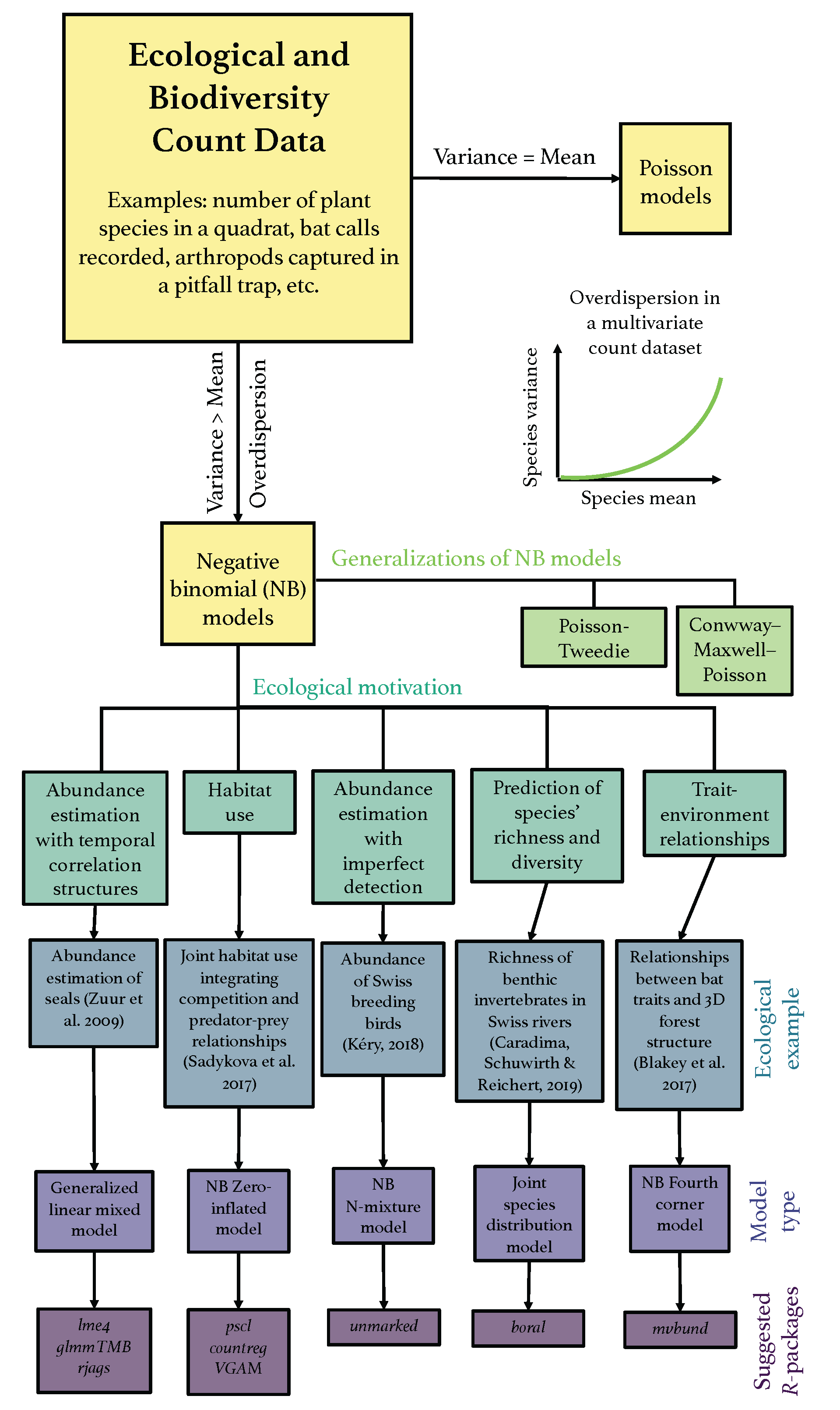
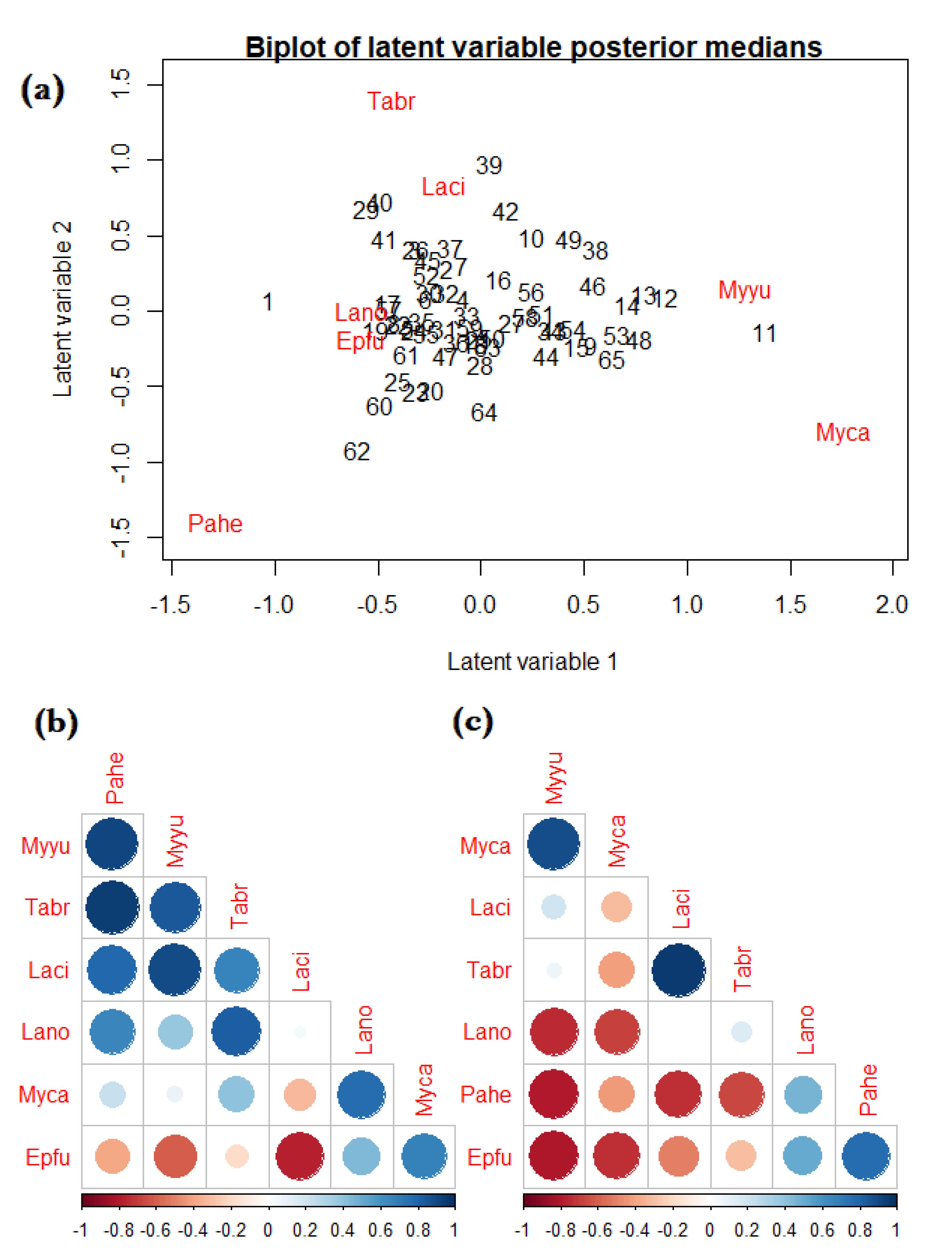
Table 1.
Parameter estimates with either 95% confidence or credible intervals when fitting a Poisson GLM, a Poisson-log-normal mixture model, a Poisson-gamma mixture model, and a Poisson–Tweedie mixture model to each species (spp.) in the bat acoustic count data. Seven bat species were recorded in oak woodlands of California, labelled by the following abbreviations: Tadarida brasiliensis (Tabr), Eptesicus fuscus (Epfu), Lasionycteris noctivagans (Lano), Lasiurus cinereus (Laci), Parastrellus hesperus (Pahe), Myotis yumanensis (Myyu), and Myotis californicus (Myca).
| Spp. | Model | |||
|---|---|---|---|---|
| Laci | Poisson | −0.38 (−0.69, −0.06) | −0.01 (−0.30, 0.29) | −0.47 (−0.83, −0.11) |
| Poisson-log-normal mixt. | −0.42 (−0.76, −0.13) | 0.01 (−0.28, 0.31) | −0.45 (−0.77, −0.12) | |
| Poisson-gamma mixt. | −0.39 (−0.73, −0.04) | 0.07 (−0.29, 0.43) | −0.46 (−0.87, −0.06) | |
| Poisson–Tweedie mixt. | −0.37 (−0.43, −0.31) | −0.00 (−0.06, 0.06 | −0.44 (−0.52, −0.37) | |
| Lano | Poisson | −0.88 (−1.30, −0.46) | 0.63 (0.19, 1.08) | −0.02 (−0.35, 0.32) |
| Poisson-log-normal mixt. | −1.09 (−2.07, −0.54) | 0.71 (0.21, 1.34) | −0.04 (−0.51, 0.34) | |
| Poisson-gamma mixt. | −0.97 (−1.50, −0.44) | 0.77 (0.08, 1.46) | 0.00 (−0.42, 0.42) | |
| Poisson–Tweedie mixt. | −0.89 (−0.98, −0.80) | 0.64 (0.55, 0.74) | −0.08 (−0.16, −0.00) | |
| Myyu | Poisson | −0.36 (−0.72, −0.01) | 0.81 (0.55, 1.07) | −1.39 (−1.72, −1.05) |
| Poisson-log-normal mixt. | −0.86 (−1.63, −0.31) | 0.46 (−0.06, 0.98) | −0.99 (−1.65, −0.43) | |
| Poisson-gamma mixt. | −0.03 (−0.47, 0.40) | 0.36 (−0.14, 0.86) | −1.02 (−1.58, −0.46) | |
| Poisson–Tweedie mixt. | 0.13 (0.07, 0.19) | 0.53 (0.45, 0.61) | −0.87 (−0.97, −0.78) | |
| Tabr | Poisson | 2.08 (1.98, 2.17) | 0.34 (0.25, 0.44) | −0.53 (−0.63, −0.42) |
| Poisson-log-normal mixt. | 0.87 (0.39, 1.29) | 0.82 (0.37, 1.33) | −0.48 (−0.93, −0.05) | |
| Poisson-gamma mixt. | 1.98 (1.64, 2.33) | 0.74 (0.15, 1.33) | −0.75 (−1.17, −0.33) | |
| Poisson–Tweedie mixt. | 2.09 (2.06, 2.12) | 0.56 (0.53, 0.59) | −0.22 (−0.25, −0.19) | |
| Epfu | Poisson | 1.39 (1.26, 1.52) | 0.30 (0.18, 0.42) | 0.62 (0.54, 0.70) |
| Poisson-log-normal mixt. | 0.07 (−0.59, 0.61) | 0.61 (0.06, 1.25) | 0.57 (0.06, 1.10) | |
| Poisson-gamma mixt. | 1.50 (1.02, 1.97) | 0.18 (−0.58, 0.93) | 0.59 (0.06, 1.12) | |
| Poisson–Tweedie mixt. | 1.58 (1.53, 1.62) | 0.36 (0.32, 0.40) | 0.31 (0.2, 0.34) | |
| Myca | Poisson | 2.16 (2.07, 2.24) | 0.31 (0.21, 0.40) | 0.14 (0.06, 0.21) |
| Poisson-log-normal mixt. | 0.64 (0.11, 1.10) | 0.32 (−0.15, 0.78) | 0.09 (−0.35, 0.55) | |
| Poisson-gamma mixt. | 2.16 (1.70, 2.62) | 0.52 (0.03, 1.02) | 0.25 (−0.24, 0.74) | |
| Poisson–Tweedie mixt. | 2.20 (2.17, 2.24) | 0.09 (0.05, 0.13) | 0.11 (0.07, 0.15) | |
| Pahe | Poisson | 0.75 (0.55, 0.94) | 0.34 (0.18, 0.51) | −0.83 (−1.04, −0.62) |
| Poisson-log-normal mixt. | −1.39 (−2.58, −0.57) | 1.16 (0.40, 2.12) | −1.32 (−2.34, −0.51) | |
| Poisson-gamma mixt. | 0.70 (0.14, 1.26) | 0.71 (−0.07, 1.49) | −1.04 (−1.75, −0.29) | |
| Poisson–Tweedie mixt. | 0.71 (0.64, 0.79) | 0.65 (0.57, 0.74) | −0.66 (−0.76, −0.57) |
Table 2.
Parameter estimates with either 95% confidence or credible intervals when fitting a negative binomial (NB GLM), zero-inflated Poisson (ZI-Poisson), and zero-inflated NB (ZI-NB) model to each species (spp.) in the bat acoustic count data. Seven bat species were recorded in oak woodlands of California, labelled by the following abbreviations: Tadarida brasiliensis (Tabr), Eptesicus fuscus (Epfu), Lasionycteris noctivagans (Lano), Lasiurus cinereus (Laci), Parastrellus hesperus (Pahe), Myotis yumanensis (Myyu), and Myotis californicus (Myca).
| Spp. | Model | |||
|---|---|---|---|---|
| Laci | NB GLM | −0.38 (−0.74, −0.01) | 0.03 (−0.33, 0.38) | −0.47 (−0.88, −0.05) |
| ZI-Poisson | 0.08 (−0.40, 0.57) | −0.05 (−0.41, 0.31) | −0.34 (−0.85, 0.17) | |
| ZI-NB | 0.08 (−0.40, 0.57) | −0.05 (−0.41, 0.31) | −0.34 (−0.85, 0.17) | |
| Lano | NB GLM | −0.91 (−1.41, −0.41) | 0.72 (0.16, 1.27) | 0.01 (−0.42, 0.43) |
| ZI-Poisson | −0.62 (−1.05, −0.19) | 0.50 (0.02, 0.97) | 0.61 (0.08, 1.14) | |
| ZI-NB | −0.64 (−1.14, −0.14) | 0.57 (−0.03, 1.17) | 0.66 (0.01, 1.31) | |
| Myyu | NB GLM | −0.02 (−0.50, 0.46) | 0.34 (−0.14, 0.81) | −0.96 (−1.53, −0.39) |
| ZI-Poisson | 0.51 (0.08, 0.94) | 0.44 (0.09, 0.78) | −1.05 (−1.46, −0.63) | |
| ZI-NB | 0.17 (−0.31, 0.65) | −0.06 (−0.63, 0.51) | −1.35 (−1.99, −0.72) | |
| Tabr | NB GLM | 1.96 (1.58, 2.34) | 0.71 (0.32, 1.11) | −0.73 (−1.13, −0.34) |
| ZI-Poisson | 2.41 (2.32, 2.51) | −0.02 (−0.13, 0.09) | −0.46 (−0.57, −0.35) | |
| ZI-NB | 2.16 (1.75, 2.58) | 0.24 (−0.36, 0.85) | −0.69 (−1.11, −0.28) | |
| Epfu | NB GLM | 1.44 (0.99, 1.88) | 0.24 (−0.21, 0.69) | 0.51 (0.07, 0.95) |
| ZI-Poisson | 1.98 (1.85, 2.12) | −0.09 (−0.27, 0.10) | 0.56 (0.47, 0.65) | |
| ZI-NB | 1.68 (1.22, 2.13) | −0.44 (−1.10, 0.22) | 0.76 (0.34, 1.18) | |
| Myca | NB GLM | 2.12 (1.67, 2.56) | 0.51 (0.06, 0.95) | 0.25 (−0.19, 0.69) |
| ZI-Poisson | 2.49 (2.40, 2.57) | 0.26 (0.17, 0.34) | 0.07 (0.00, 0.14) | |
| ZI-NB | 2.12 (1.67, 2.56) | 0.51 (−0.02, 1.04) | 0.25 (−0.25, 0.74) | |
| Pahe | NB GLM | 0.62 (0.03, 1.21) | 0.67 (0.05, 1.29) | −1.08 (−1.75, −0.41) |
| ZI-Poisson | 1.84 (1.63, 2.04) | −0.23 (−0.42, −0.03) | −0.55 (−0.79, −0.31) | |
| ZI-NB | 1.43 (0.53, 2.32) | −0.27 (−1.09, 0.55) | −0.81 (−1.81, 0.18) |
Table 3.
A selective list of R-packages for fitting various traditional and modern negative binomial (NB) models described in the main text. We denote as s the number of species/taxa, n the number of sampling units (e.g., sites), and p the number of covariates. Note that generic Bayesian MCMC packages such as the rjags and R2jags R-packages can also be used to fit many of the models listed below, with some additional coding required for specifying the NB likelihood. Indeed, some of the modern NB models discussed in Section 3 either do not have currently associated R-packages, or require bespoke R-code. Furthermore, some of the packages listed can fit multiple types of NB models (e.g., the gamlss package can also fit NB GLMs and GAMs).
| Model: | Modelling Usage and Notes: | R-Package(s): | Common Function: |
|---|---|---|---|
| Generalised linear model (GLM) | Single species () | MASS | glm.nb() |
| Generalised additive model (GAM) | Smoothing | mgcv | gam(family = nb()) |
| gamlss | gamlss(family = NBI) | ||
| Generalised linear mixed model (GLMM) | Random/mixed effects | lme4 | glmer.nb() |
| glmmTMB/glmmadmb | glmmTMBfamily = nbinom2() | ||
| Generalised additive mixed model | mgcv | gamm(family = nb()) | |
| GLM with regularisation penalties | High-dimension | glmnet | glmnet(family = negative.binomial) |
| GLMM with regularisation penalties | rpql | rpql(family = "nb2") | |
| Species distribution model | Stacked SDM () | mvabund | manyglm(family = "negative.binomial") |
| Stacked and Reduced-rank SDMs/GAMs | VGAM | vglm(family = negbinomial()) | |
| Joint species distribution model | (Residual) correlation across species | boral | boral(family = "negative.binomial") |
| gllvm | gllvm(family = "negative.binomial") | ||
| Poisson-log-normal mixture model | HierarchicalGOF | pois.overd.no.spat() | |
| Poisson-gamma mixture model | bsamGP | gblr(family = "poisson.gamma") | |
| Poisson–Tweedie mixture model | ptmixed | ptglm() | |
| Zero-inflated GLM | pscl/countreg | zeroinfl(dist = "negbin") | |
| VGAM | vglm(family = zinegbin()) | ||
| gamlss | family = ZIP()/ZINBI() | ||
| Zero-truncated GLM | countreg | zerotrunc(dist = "negbin") | |
| VGAM | vglm(family = posnegbinom()) | ||
| gamlss.tr | gen.trun(family = "PO") | ||
| N-mixture models | Imperfect detection | unmarked | pcount(mixture = "NB") |
| Generalised multinomial N-mixture | Three hierarchical levels | unmarked | gmultmix(mixture = "NB") |
| Hierarchical distance sampling | unmarked | gdistsamp(mixture = "NB") |
Publisher’s Note: MDPI stays neutral with regard to jurisdictional claims in published maps and institutional affiliations. |
© 2022 by the authors. Licensee MDPI, Basel, Switzerland. This article is an open access article distributed under the terms and conditions of the Creative Commons Attribution (CC BY) license (https://creativecommons.org/licenses/by/4.0/).
Share and Cite
MDPI and ACS Style
Stoklosa, J.; Blakey, R.V.; Hui, F.K.C. An Overview of Modern Applications of Negative Binomial Modelling in Ecology and Biodiversity. Diversity 2022, 14, 320. https://doi.org/10.3390/d14050320
AMA Style
Stoklosa J, Blakey RV, Hui FKC. An Overview of Modern Applications of Negative Binomial Modelling in Ecology and Biodiversity. Diversity. 2022; 14(5):320. https://doi.org/10.3390/d14050320
Chicago/Turabian StyleStoklosa, Jakub, Rachel V. Blakey, and Francis K. C. Hui. 2022. "An Overview of Modern Applications of Negative Binomial Modelling in Ecology and Biodiversity" Diversity 14, no. 5: 320. https://doi.org/10.3390/d14050320
Note that from the first issue of 2016, this journal uses article numbers instead of page numbers. See further details here.