Phylogenetic Signal of Threatening Processes among Hylids: The Need for Clade-Level Conservation Planning

Abstract
:
1. Introduction
2. Methods
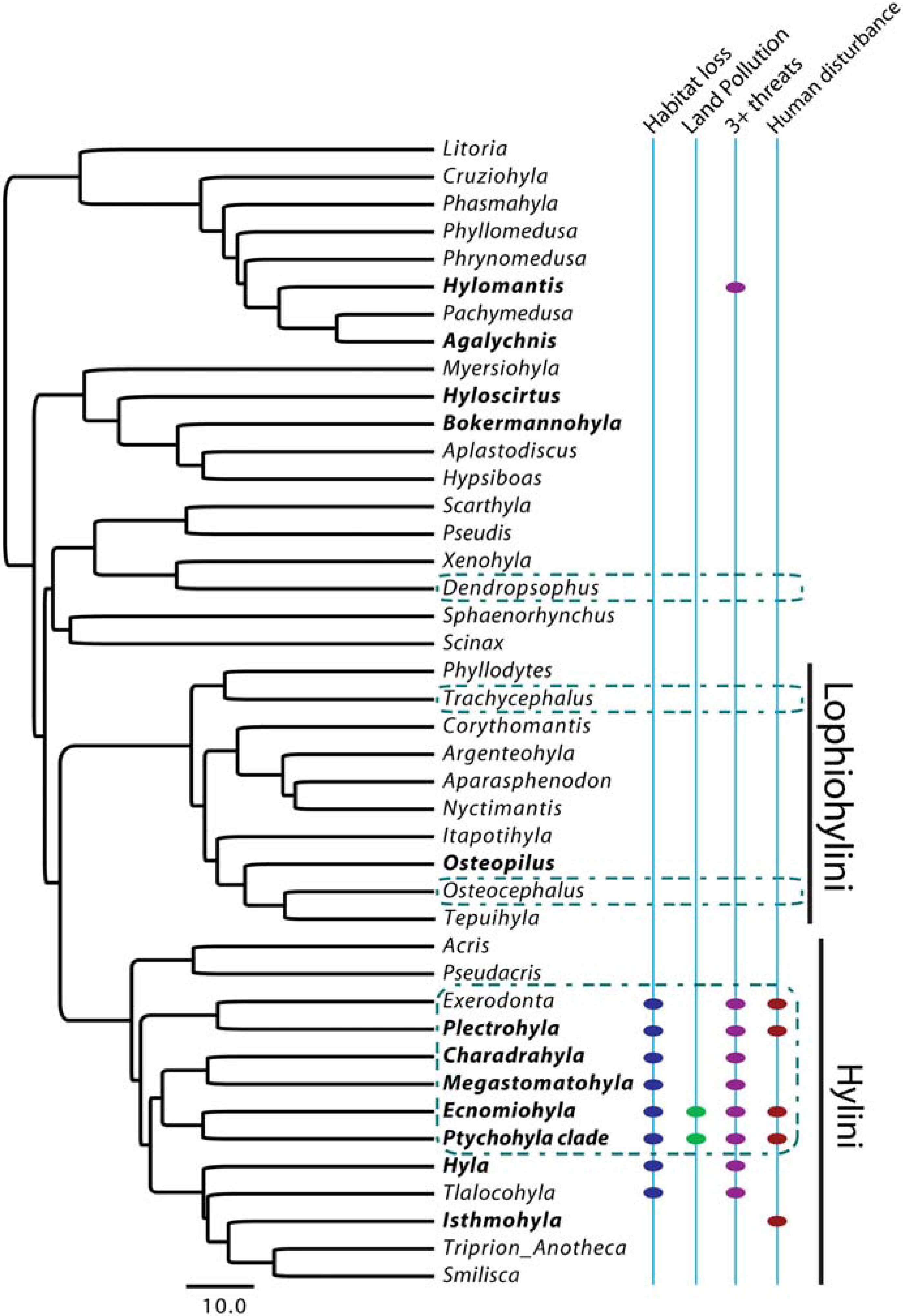
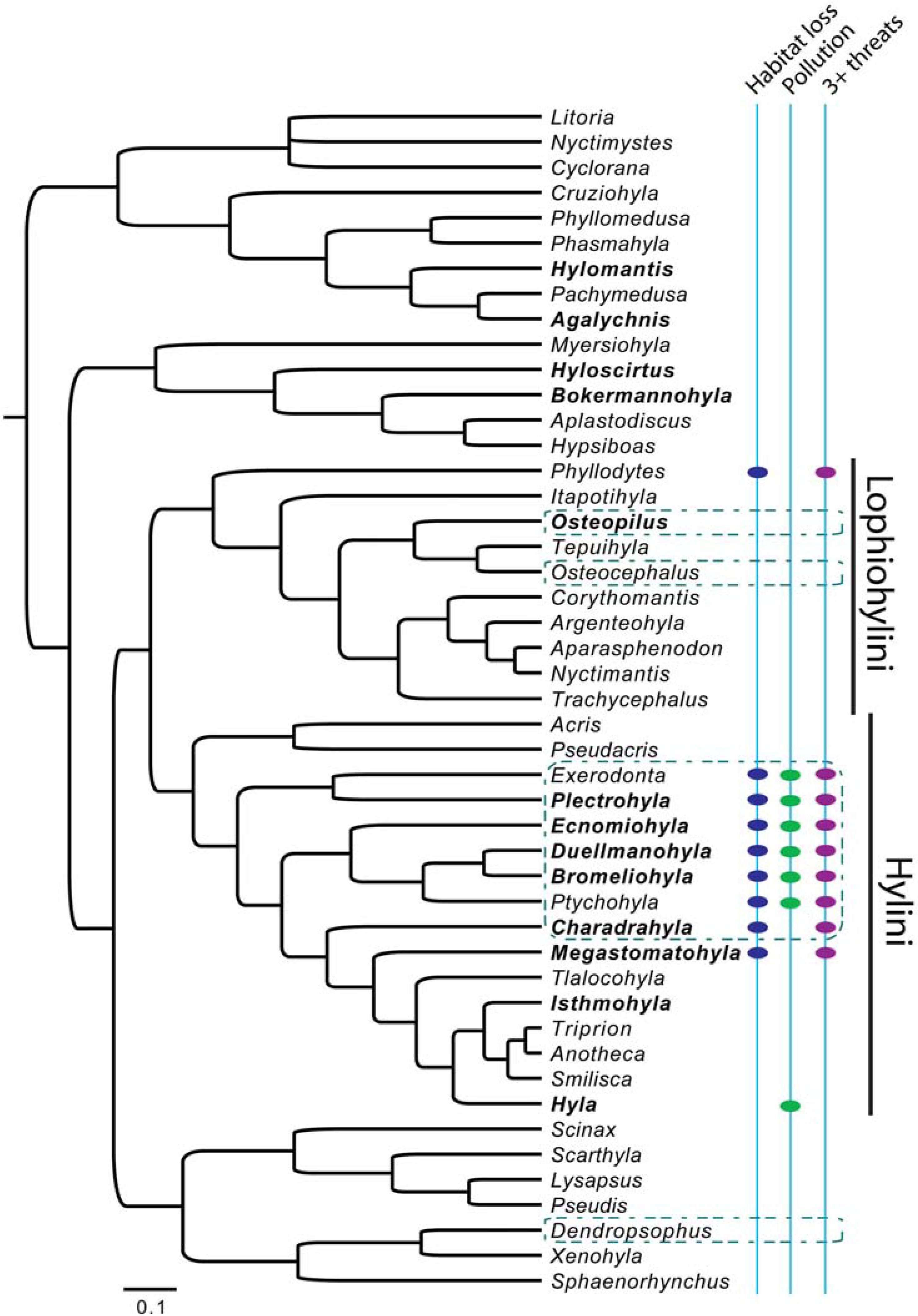
2.1. Phylogenies
2.2. Comparative Data
2.3. Phylogenetic Comparative Methods

2.3.1. Applying PCMs that do not directly assume an evolutionary model
 . Alpha is also considered an estimate of the rate of trait evolution [31].
2.3.2. PCMs based on Brownian Motion

2.3.3. PCMs based on Brownian Motion with evolutionary constraints
2.3.4. A PCM incorporating evolutionary constraints


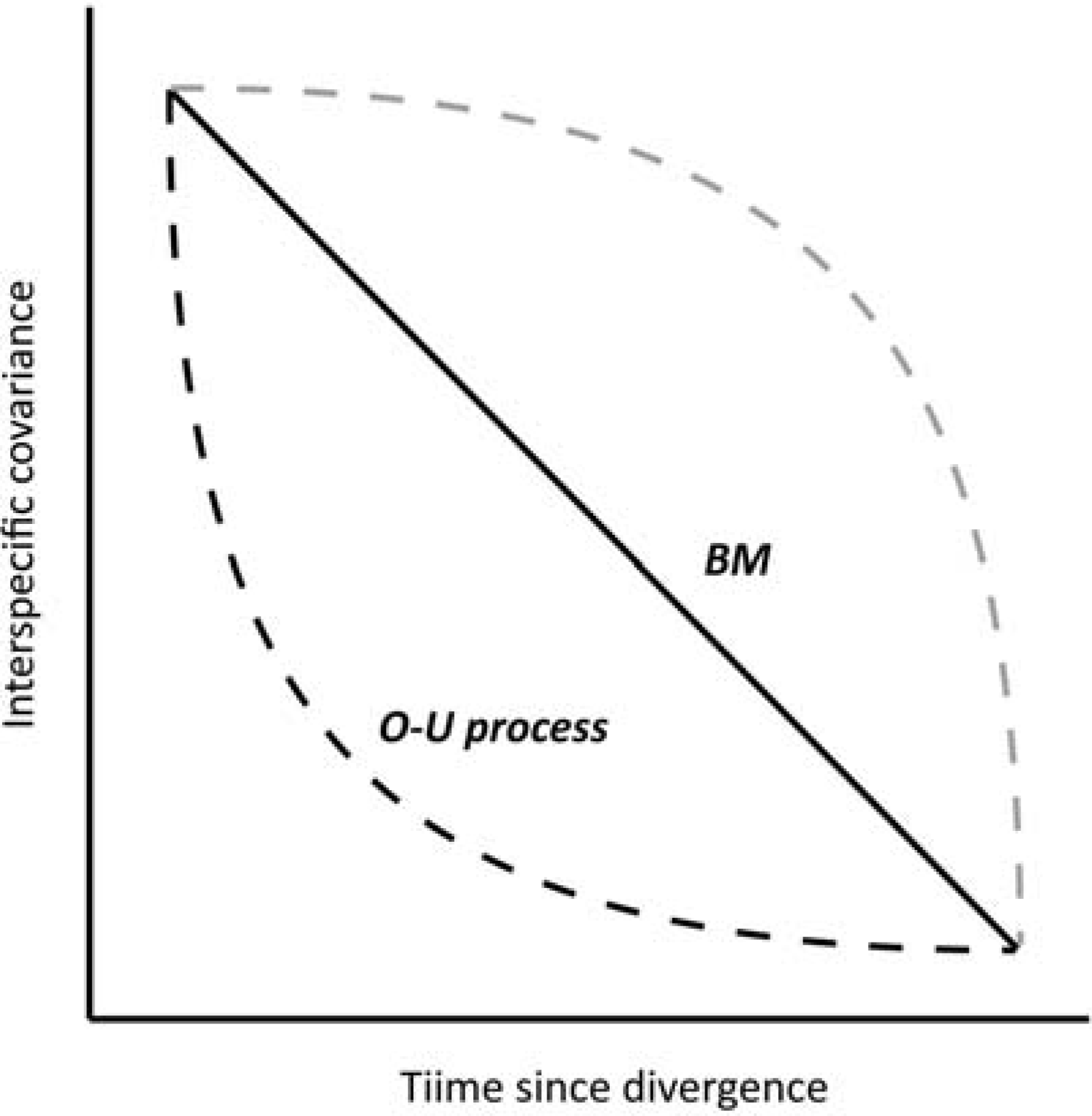
 is the rate of evolutionary divergence through time, τi is the node-to-tip branch length of species i, and the shared branch length between tips i and j is represented by τij. Additionally, the d parameter can be used to test the statistical adequacy of original branch lengths by asking, does the tree fit the trait data? Thus, the diagnostic use of d gives information about the degree of phylogenetic structure. As a diagnostic test for the K-statistic and randomization test for signal, the d-transformed tree MSEs were consistently lower than the MSE of the original tree.
 3. Results

| Threat component | Blomberg et al. | ||||||
|---|---|---|---|---|---|---|---|
| P randomization test of signal† | d | P d = 0 | K-statistic¥ | Diagnostic test‡‡ | |||
| Threatened status | 0.33 (0.21) | 0.3471* | 0.0420 | 0.6559 | 0.0460 | 0.9823 | sig |
| Threatened + Data Deficient status | 0.25 (0.23) | 0.0000* | 0.0290 | 0.7117 | 0.0510 | 0.9869 | sig |
| Enigmatic decline | ns | 0.0069 | 0.0660 | 1.1579 | 0.0290 | 0.6774 | 1-tailed sig |
| 2+ types of threat | 0.38 (0.21) | 0.4769 | 0.0300 | 0.6868 | 0.0480 | 0.9935 | sig |
| 3+ types of threat | 0.28 (0.23) | 0.2474* | sig | ||||
| All Habitat loss (HL) | 0.44 (0.20) | 0.5848 | 0.0340 | 0.7159 | 0.0430 | 0.9919 | sig |
| Agriculture HL | 0.29 (0.23) | 0.3516* | sig | ||||
| Extraction HL | 0.52 (0.18) | 1.1000‡ | sig | ||||
| Infrastructure HL | 0.32 (0.23) | 0.2672* | sig | ||||
| All Pollution | ns | 0.1506** | ns | ||||
| Land pollution | 0.41 (0.20) | 1.1000‡ | 0.5890 | n/s | 0.5600 | ns | |
| Water pollution | ns | 0.0931* | ns | ||||
| Human disturbance | 0.33 (0.21) | 0.4796 | 0.3070 | n/a | 0.1280 | ns | |
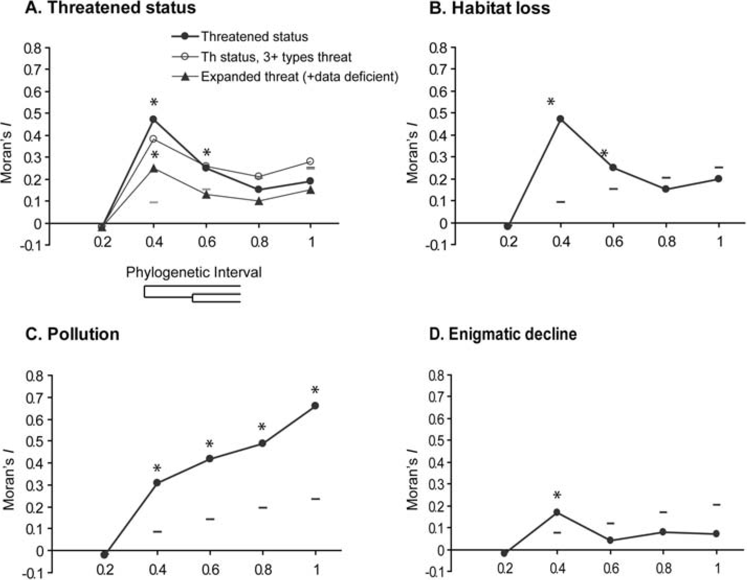
3.1. Moran’s I

3.2. Autoregressive Method

3.3. Pagel’s λ
3.4. Blomberg’s Randomization Test of Signal and K-Statistic
3.5. Blomberg’s d
4. Discussion
4.1. Phylogenetic Signal in Threatening Processes
4.2. Interpreting Phylogenetic Signal
4.3. Evolutionary Models in Phylogenetic Comparative Methods
4.4. Considering Effects of Phylogeography
4.5. Conservation Implications
| Genus | Enigmatic Decline | Threatened | HL | Pollution | B.d. | DD | Distribution of threatened species |
|---|---|---|---|---|---|---|---|
| Plectrohyla (41) | 17 | 38 | 38 | 12 | 6 (32) | 2 | Guatemala, Mexico, Honduras, El Salvador |
| Ptychohyla clade (23) | 5 | 20 | 20 | 11 | 5 (15) | 2 | Guatemala, Mexico, Honduras, Nicaragua, Panama, Costa Rica, El Salvador |
| Isthmohyla (14) | 6 | 10 | 9 | 6 | 1 (6) | 2 | Costa Rica, Panama, Honduras |
| Ecnomiohyla (10) | 1 | 7 | 7 | 2 | 0 (1) | 1 | Mexico, Costa Rica, Panama, Nicaragua, Guatemala, Colombia, Ecuador, Honduras |
| Exerodonta (11) | 0 | 7 | 7 | 1 | 1 (3) | 2 | Honduras, Mexico, Guatemala |
| Charadrahyla (5) | 1 | 5 | 5 | 0 | 1 (2) | 0 | Mexico |
| Megastomatohyla (4) | 1 | 4 | 4 | 0 | 0 | 0 | Mexico |
| Hyla (44) | 1 | 3 | 3 | 2 | 0 | 13 | Guatemala, Bolivia, Mexico |
| Tlalocohyla (4) | 0 | 1 | 1 | 0 | 0 | 0 | Mexico |
Acknowledgements
References
- Corey, S.J.; Waite, T.A. Phylogenetic autocorrelation of extinction threat in globally imperiled amphibians. Divers. Distrib. 2008, 14, 614–629. [Google Scholar] [CrossRef]
- Stuart, S.N.; Chanson, J.S.; Cox, N.A.; Young, B.E.; Rodrigues, A.S.L.; Fischman, D.L.; Waller, R.W. Status and trends of amphibian declines and extinctions worldwide. Science 2004, 306, 1783–1786. [Google Scholar] [CrossRef]
- Pounds, A.J.; Bustamante, M.; Coloma, L.; Consuegra, J.; Fogden, M.; Foster, P.; La Marca, E.; Masters, K.; Merino-Viteri, A.; Puschendorf, R.; Ron, S.; Sánchez-Azofeifa, G.; Still, C.; Young, B. Widespread amphibian extinctions from epidemic disease driven by global warming. Nature 2006, 439, 161–167. [Google Scholar] [CrossRef]
- Lips, K.R.; Mendelson, J.R., III; Muńoz-Alonso, A. Amphibian population declines in montane southern Mexico: Resurveys of historical localities. Biol. Conserv. 2004, 119, 555–564. [Google Scholar] [CrossRef]
- Lips, K.R.; Burrowes, P.A.; Mendelson, J.R.I.; Parra-Olea, G. Amphibian declines in Latin America: Widespread population declines, extinctions, and impacts. Biotropica 2006, 37, 163–165. [Google Scholar]
- Lips, K.R.; Reeve, J.D.; Witters, L.R. Ecological traits predicting amphibian population declines in Central America. Conserv. Biol. 2003, 17, 1078–1088. [Google Scholar] [CrossRef]
- International Union for Conservation of Nature (IUCN). IUCN Red List of Threatened Species. 2008. Available online: http://www.iucnredlist.org (accessed on 20 April 2009).
- Corey, S.J. Understanding Amphibian Vulnerability to Extinction: A Phylogenetic and Spatial Approach. In Ph.D. Thesis; The Ohio State University: Columbus, OH, USA, 2009. [Google Scholar]
- Faivovich, J.; Haddad, C.F.B.; Garcia, P.C.A.; Frost, D.R. Systematic review of the frog family Hylidae, with special reference to Hylinae: Phylogenetic analysis and taxonomic revision. Bull. Am. Mus. Nat. Hist. 2005, 294, 240. [Google Scholar]
- Smith, S.A.; Arif, S.; de Oca, A.; Wiens, J. A phylogenetic hot spot for evolutionary novelty in Middle American treefrogs. Evolution 2007, 61, 2075–2085. [Google Scholar] [CrossRef]
- Frost, D.R. Amphibian Species of the World: An Online Reference. Version 5.3. American Museum of Natural History: New York, NY, USA, 2009. Available online: http://research.amnh.org/herpetology/amphibia/ (accessed on 20 April 2009).
- Wiens, J.; Graham, C.H.; Moen, D.S.; Smith, S.A.; Reeder, T. Evolutionary and ecological causes of the latitudinal diversity gradient in hylid frogs: Treefrog trees unearth the roots of high tropical diversity. Am. Nat. 2006, 168, 579–596. [Google Scholar] [CrossRef]
- Smith, S.A.; de Oca, A.; Reeder, T.; Wiens, J. A phylogenetic perspective on elevational species richness patterns in Middle American treefrogs: Why so few species in lowland tropical rainforests? Evolution 2007, 61, 1188–1207. [Google Scholar] [CrossRef]
- Frost, D.R.; Grant, T.; Faivovich, J.; Bain, R.; Haas, A.; Haddad, C.; de Sa, R.; Channing, A.; Wilkinson, M.; Donnellan, S. The amphibian tree of life. Bull. Am. Mus. Nat. Hist. 2006, 297, 370. [Google Scholar]
- Aguiar, O., Jr.; Bacci, M.; Lima, A.P.; Rossa-Feres, D.C.; Haddad, C.F.B.; Recco-Pimentel, S.M. Phylogenetic relationships of Pseudis and Lysapsus (Anura, Hylidae, Hylinae) inferred from mitochondrial and nuclear gene sequences. Cladistics 2007, 23, 455–463. [Google Scholar] [CrossRef]
- Martins, E.P. COMPARE 4.6b: Computer Programs for the Statistical Analysis of Comparative Data. 2004. Available online: http://compare.bio.indiana.edu (accessed on 15 November 2007).
- Rambaut, A.; Charleston, M. TreeEdit. 2001. Available online: http://tree.bio.ed.ac.uk/software/treeedit (accessed on 13 July 2006).
- Sanderson, M.J. A nonparametric approach to estimating divergence times in the absence of rate constancy. Mol. Biol. Evol. 1997, 14, 1218–1231. [Google Scholar] [CrossRef]
- Mace, G.; Collar, N.; Gaston, K.; Hilton-Taylor, C.; Akçakaya, H.; Leader-Williams, N.; Milner-Gulland, E.; Stuart, S. Quantification of extinction risk: IUCN’s system for classifying threatened species. Conserv. Biol. 2008, 22, 1424–1442. [Google Scholar] [CrossRef]
- International Union for Conservation of Nature (IUCN); Conservation International; NatureServe. Global Amphibian Assessment. (formerly http://www.globalamphibians.org) (accessed on 13 February 2009).
- Lockwood, J.L.; Russell, G.J.; Gittleman, J.L.; Daehler, C.C.; McKinney, M.M.; Purvis, A. A metric for analyzing taxonomic patterns of extinction risk. Conserv. Biol. 2002, 16, 1137–1142. [Google Scholar] [CrossRef]
- Smith, K.; Sax, D.; Lafferty, K. Evidence for the role of infectious disease in species extinction and endangerment. Conserv. Biol. 2006, 20, 1349–1357. [Google Scholar] [CrossRef]
- Bielby, J.; Cooper, N.; Cunningham, A.; Garner, T.; Purvis, A. Predicting susceptibility to future declines in the world’s frogs. Conserv. Lett. 2008, 1, 82–90. [Google Scholar] [CrossRef]
- Ord, T.; Martins, E. Tracing the origins of signal diversity in anole lizards: Phylogenetic approaches to inferring the evolution of complex behaviour. Anim. Behav. 2006, 71, 1411–1429. [Google Scholar] [CrossRef]
- Blomberg, S.P.; Garland, T.; Ives, A.R. Testing for phylogenetic signal in comparative data: Behavioral traits are more labile. Evolution 2003, 57, 717–745. [Google Scholar] [CrossRef]
- Diniz-Filho, J.A.F. Phylogenetic autocorrelation under distinct evolutionary processes. Evolution 2001, 55, 1104–1109. [Google Scholar] [CrossRef]
- Martins, E.; Diniz-Filho, J.A.F.; Housworth, E. Adaptive constraints and the phylogenetic comparative method: a computer simulation test. Evolution 2002, 56, 1–13. [Google Scholar] [CrossRef]
- Moran, P.A.P. Notes on continuous stochastic phenomena. Biometrika 1950, 37, 17–23. [Google Scholar] [CrossRef]
- Cheverud, J.M.; Dow, M.M.; Leutenegger, W. The quantitative assessment of phylogenetic constraints in comparative analyses: Sexual dimorphism in body weight among primates. Evolution 1985, 39, 1335–1351. [Google Scholar] [CrossRef]
- Gittleman, J.L.; Kot, M. Adaptation: Statistics and a null model for estimating phylogenetic effects. Syst. Zool. 1990, 39, 227–241. [Google Scholar] [CrossRef]
- Martins, E.P.; Hansen, T.F. The statistical analysis of interspecific data: A review and evaluation of phylogenetic comparative methods. In Phylogenies and the Comparative Method in Animal Behavior; Martins, E.P., Ed.; Oxford University Press: Oxford, UK, 1996; pp. 22–75. [Google Scholar]
- Pagel, M. Inferring the historical patterns of biological evolution. Nature 1999, 401, 877–884. [Google Scholar] [CrossRef]
- Garland, T., Jr.; Harvey, P.H.; Ives, A.R. Procedures for the analysis of comparative data using phylogenetically independent contrasts. Syst. Biol. 1992, 41, 18–32. [Google Scholar] [CrossRef]
- Midford, P.E.; Garland, T., Jr.; Maddison, W.P. PDAP Package of Mesquite, Version 1.07. 2005. Available online: http://mesquiteproject.org (accessed on 15 November 2008).
- Maddison, W.P.; Maddison, D.R. Mesquite: A Modular System for Evolutionary Analysis, Version 2.6. 2009. Available online: http://mesquiteproject.org (accessed on 13 February 2009).
- Diaz-Uriarte, R.; Garland, T., Jr. Effects of branch length errors on the performance of phylogenetically independent contrasts. Syst. Biol. 1998, 47, 654–672. [Google Scholar] [CrossRef]
- Butler, M.A.; King, A.A. Phylogenetic comparative analysis: A modeling approach for adaptive evolution. Am. Nat. 2004, 164, 683–695. [Google Scholar] [CrossRef]
- Purvis, A. Phylogenetic approaches to the study of extinction. Ann. Rev. Ecol. Evol. Syst. 2008, 39, 301–319. [Google Scholar] [CrossRef]
- Owens, I.; Bennett, P.M. Ecological basis of extinction risk in birds: Habitat loss versus human persecution and introduced predators. Proc. Natl. Acad. Sci. USA 2000, 97, 12144–12148. [Google Scholar] [CrossRef]
- Davidson, A.D.; Hamilton, M.J.; Boyer, A.G.; Brown, J.H.; Ceballos, G. Multiple ecological pathways to extinction in mammals. Proc. Natl. Acad. Sci. USA 2009, 106, 10702–10705. [Google Scholar] [CrossRef]
- Loyola, R.; Becker, C.G.; Kubota, U.; Haddad, C.F.B.; Fonseca, C.R.; Lewinsohn, T.M. Hung out to dry: Choice of priority ecoregions for conserving threatened neotropical anurans depends on life-history traits. PLoS One 2008, 3, e2120. [Google Scholar]
- Fortin, M.J.; Dale, M. Spatial pattern. In Spatial Analysis: A Guide for Ecologists; Cambridge University Press: Cambridge, UK, 2005; pp. 6–10. [Google Scholar]
- Russell, G.J.; Brooks, T.M.; Mckinney, M.M.; Anderson, G.C. Present and future taxonomic selectivity in Bird and Mammal extinctions. Conserv. Biol. 1998, 12, 1365–1376. [Google Scholar] [CrossRef]
- Mace, G.M.; Gittleman, J.L.; Purvis, A. Preserving the tree of life. Science 2003, 300, 1707–1709. [Google Scholar] [CrossRef]
- McKinney, M.L. Extinction vulnerability and selectivity: Combining ecological and paleontological views. Ann. Rev. Ecol. Syst. 1997, 28, 495–516. [Google Scholar] [CrossRef]
- Gardner, T.; Barlow, J.; Peres, C. Paradox, presumption and pitfalls in conservation biology: The importance of habitat change for amphibians and reptiles. Biol. Conserv. 2007, 138, 166–179. [Google Scholar] [CrossRef]
- Schiesari, L.; Grillitsch, B.; Grillitsch, H. Biogeographic biases in research and their consequences for linking amphibian declines to pollution. Conserv. Biol. 2005, 21, 465–471. [Google Scholar]
- Kerby, J.L.; Richards-Hrdlicka, K.L.; Storfer, A.; Skelly, D.K. An examination of amphibian sensitivity to environmental contaminants: are amphibians poor canaries? Ecol. Lett. 2010, 13, 60–67. [Google Scholar] [CrossRef]
Appendix
Results of the Analysis with the Faivovich Phylogeny
| Threat Component | ρ (±90% CI) |
|---|---|
| Threatened status | 0.43 (0.197) |
| Threatened + Data deficient status | 0.29 (0.230) |
| Enigmatic decline | ns |
| 2+ types of threat | 0.44 (0.197) |
| 3+ types of threat | 0.45 (0.110) |
| All Habitat loss | 0.44 (0.197) |
| All Pollution | 0.52 (0.165) |

| Category of Threat | P Randomization Test of Signal* | d | P for d= 0 | P for d= 1 | Expected MSE0/MSE | Observed MSE0/MSE | K | MSE Star | MSE Original | MSE O-U |
|---|---|---|---|---|---|---|---|---|---|---|
| Threatened status | 0.0420 | 0.6559 | 0.0460 | 0.3900 | 1.0472 | 1.0287 | 0.9823 | 0.1077 | 0.1116 | 0.1050 |
| 2+ types of threat | 0.0300 | 0.6868 | 0.0480 | 0.4120 | 1.0574 | 1.0506 | 0.9935 | 0.1065 | 0.1093 | 0.1025 |
| All Habitat loss | 0.0340 | 0.7159 | 0.0430 | 0.4260 | 0.0681 | 1.0594 | 0.9919 | 0.1172 | 0.1183 | 0.1119 |
| Land pollution | 0.5890 | 0.5600 | ||||||||
| Enigmatic decline | 0.0660 | 1.1579 | 0.0290 | 0.0780 | 1.9534 | 1.3232 | 0.6774 | 0.0139 | 0.0141 | 0.0108 |
| Threatened + Data deficient status | 0.0290 | 0.7117 | 0.0510 | 0.4290 | 1.0664 | 1.0525 | 0.9869 | 0.1216 | 0.1228 | 0.1179 |
| Human disturbance | 0.3070 | 0.1280 |
© 2010 by the authors; licensee Molecular Diversity Preservation International, Basel, Switzerland. This article is an open-access article distributed under the terms and conditions of the Creative Commons Attribution license (http://creativecommons.org/licenses/by/3.0/).
Share and Cite
Corey, S.J. Phylogenetic Signal of Threatening Processes among Hylids: The Need for Clade-Level Conservation Planning. Diversity 2010, 2, 142-162. https://doi.org/10.3390/d2020142
Corey SJ. Phylogenetic Signal of Threatening Processes among Hylids: The Need for Clade-Level Conservation Planning. Diversity. 2010; 2(2):142-162. https://doi.org/10.3390/d2020142
Chicago/Turabian StyleCorey, Sarah J. 2010. "Phylogenetic Signal of Threatening Processes among Hylids: The Need for Clade-Level Conservation Planning" Diversity 2, no. 2: 142-162. https://doi.org/10.3390/d2020142
APA StyleCorey, S. J. (2010). Phylogenetic Signal of Threatening Processes among Hylids: The Need for Clade-Level Conservation Planning. Diversity, 2(2), 142-162. https://doi.org/10.3390/d2020142