Predicting Climate Change Impacts to the Canadian Boreal Forest

Abstract

Climate change is expected to alter temperature, precipitation, and seasonality with potentially acute impacts on Canada’s boreal. In this research we predicted future spatial distributions of biodiversity in Canada’s boreal for 2020, 2050, and 2080 using indirect indicators derived from remote sensing and based on vegetation productivity. Vegetation productivity indices, representing annual amounts and variability of greenness, have been shown to relate to tree and wildlife richness in Canada’s boreal. Relationships between historical satellite-derived productivity and climate data were applied to modelled scenarios of future climate to predict and map potential future vegetation productivity for 592 regions across Canada. Results indicated that the pattern of vegetation productivity will become more homogenous, particularly west of Hudson Bay. We expect climate change to impact biodiversity along north/south gradients and by 2080 vegetation distributions will be dominated by processes of seasonality in the north and a combination of cumulative greenness and minimum cover in the south. The Hudson Plains, which host the world’s largest and most contiguous wetland, are predicted to experience less seasonality and more greenness. The spatial distribution of predicted trends in vegetation productivity was emphasized over absolute values, in order to support regional biodiversity assessments and conservation planning.

1. Introduction

Latitudes north of 40° are expected to experience the greatest temperature increases due to climate change [1]. In northern locations, impacts of climate change are expected to be acute and the ecological response to climate change will vary spatially [2]. Alterations to biodiversity are one of the expected responses to climate change [3]. Most commonly, climate change is expected to reduce climatic constraints to plant growth [4]. Warmer, wetter conditions will result in increased vegetation productivity, which has been demonstrated as an indirect indicator of biodiversity that correlates with geographic variation in species richness [5].

Canada’s boreal is a unique northern environment where climate change is expected to have some of its largest impacts (e.g., [2,3,6,7]. To date, changes to fire regimes [8] and periodicity and impacts of insect infestations [9] have been documented and are unevenly distributed due to their dependence on local factors including terrain and moisture conditions. A large and ecologically continuous landscape [10], Canada’s boreal has been documented as essential for maintaining biodiversity [11,12,13]. Using measures of forest contiguity and functional traits, 80% of Canada’s boreal occurs in contiguous blocks [14,15] and provides a range of ecosystem services, such as carbon storage [16] within a stable ecosystem [17].

Over expansive areas such as Canada’s boreal, biodiversity management requires large area mapping and monitoring of vegetation conditions. In general, highly productive areas are hypothesized to support more species by providing ample food and habitat resources to partition among species [18,19]. Research also indicates that migratory fauna respond to seasonal productive pulses, whereas resident fauna preferentially select areas of consistent annual productivity, demonstrating the importance of modelling integrated annual (and variance) measures of vegetation production [20].

Remote sensing-derived productivity indicators have been shown to provide indirect representations of biodiversity in several areas [5,20,21,22,23,24,25], including Canada’s boreal [26] and have been related to vegetation and wildlife species richness [26,27,28]. In addition to providing spatially extensive and continuous data for indirect mapping of biodiversity indicators, remote sensing archives are temporally rich. Historical data from the Advanced Very High Resolution Radiometer (AVHRR) satellite sensor have been used to map Canada’s vegetation productivity annually, from 1981–2007, at a 1 km spatial resolution using imagery captured monthly [29].

In our research, productivity mapping is based on the fraction of photosynthetically active radiation (fPAR) absorbed by a vegetated canopy [23,29]. Radiation spanning the visible electromagnetic spectrum from 400–700 nm is absorbed by plant pigments for photosynthesis. Integrating maximum monthly absorption can be used as a proxy for production, as growth is indicative of the rate at which vegetation absorbs energy [19]. For an area where fPAR remains high over a growing season, high vegetation productivity can be inferred [23].

Several studies have documented a general link between vegetation productivity and biodiversity [5,28,30,31]. Though the associations are nuanced and complex, at the most simplistic level increased vegetation productivity generates more energy available to support species and therefore higher biodiversity [32,33,34,35,36,37]. More specifically, derivatives of fPAR have been related to species distribution and diversity [28,38].

Given the links between climate, vegetation, and ultimately biodiversity, quantifying possible responses of biodiversity to climate change provides important information to decision makers. Through integration with historical climate data, temporal archives of vegetation productivity provide an opportunity to quantify past trends between climate and productivity, and indirectly biodiversity [39]. Modelled relationships between historical climate and productivity data can be integrated with future climate scenarios to map possible future spatial distributions of vegetation productivity. For instance, climate modelling has been used to show that vegetation primary productivity may increase due to climate change [40].

The goal of this research was to understand how climate change might alter vegetation productivity in Canada’s boreal forest, and in turn how biodiversity will be impacted. To meet this goal we:

(1).

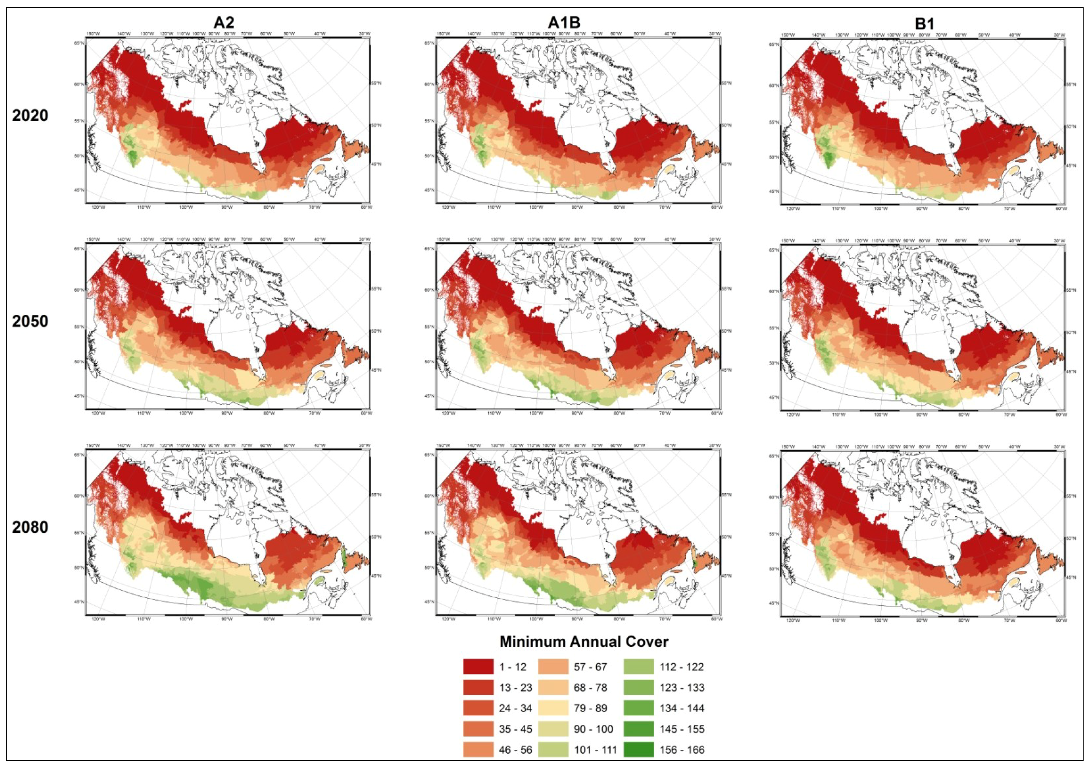
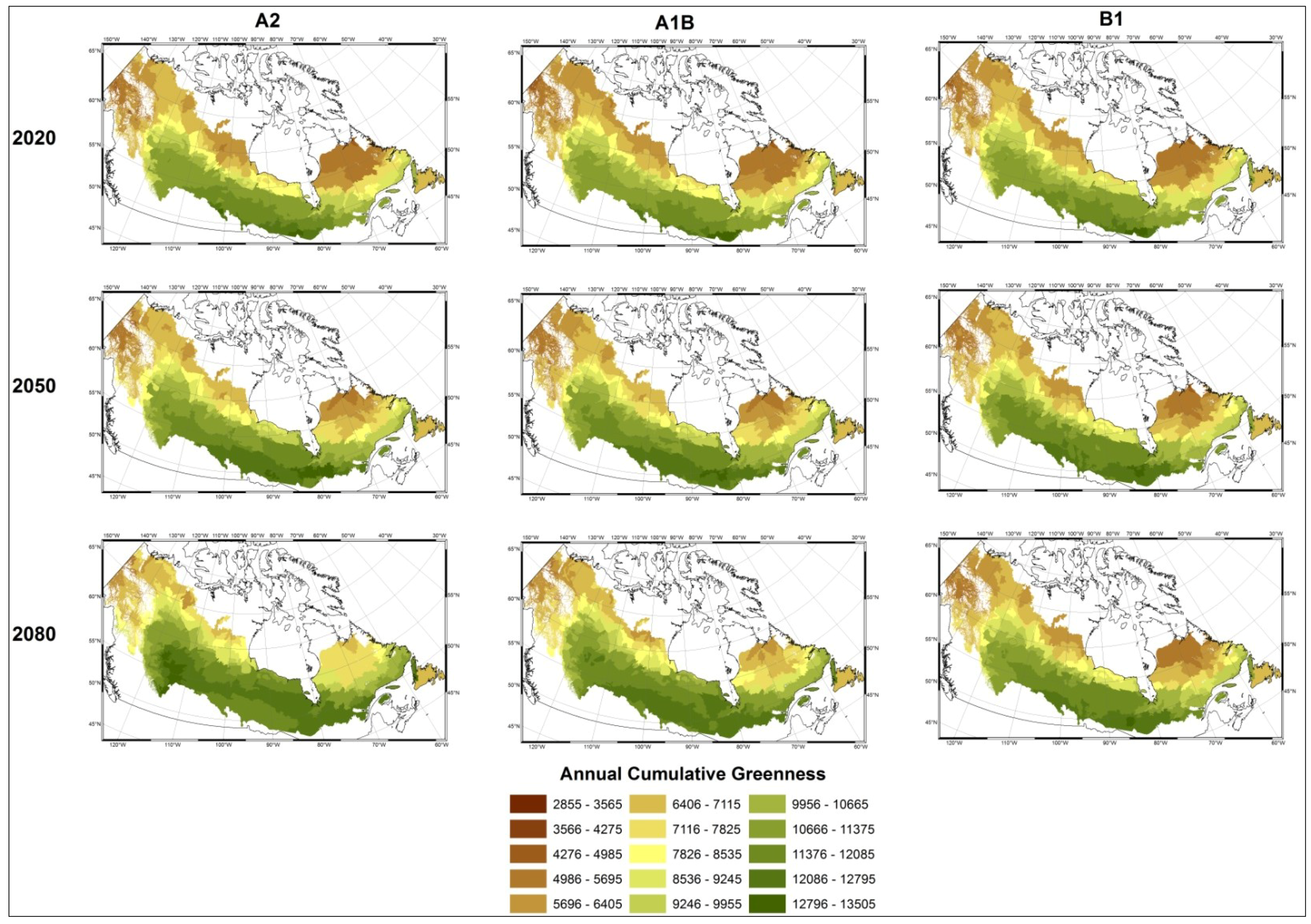
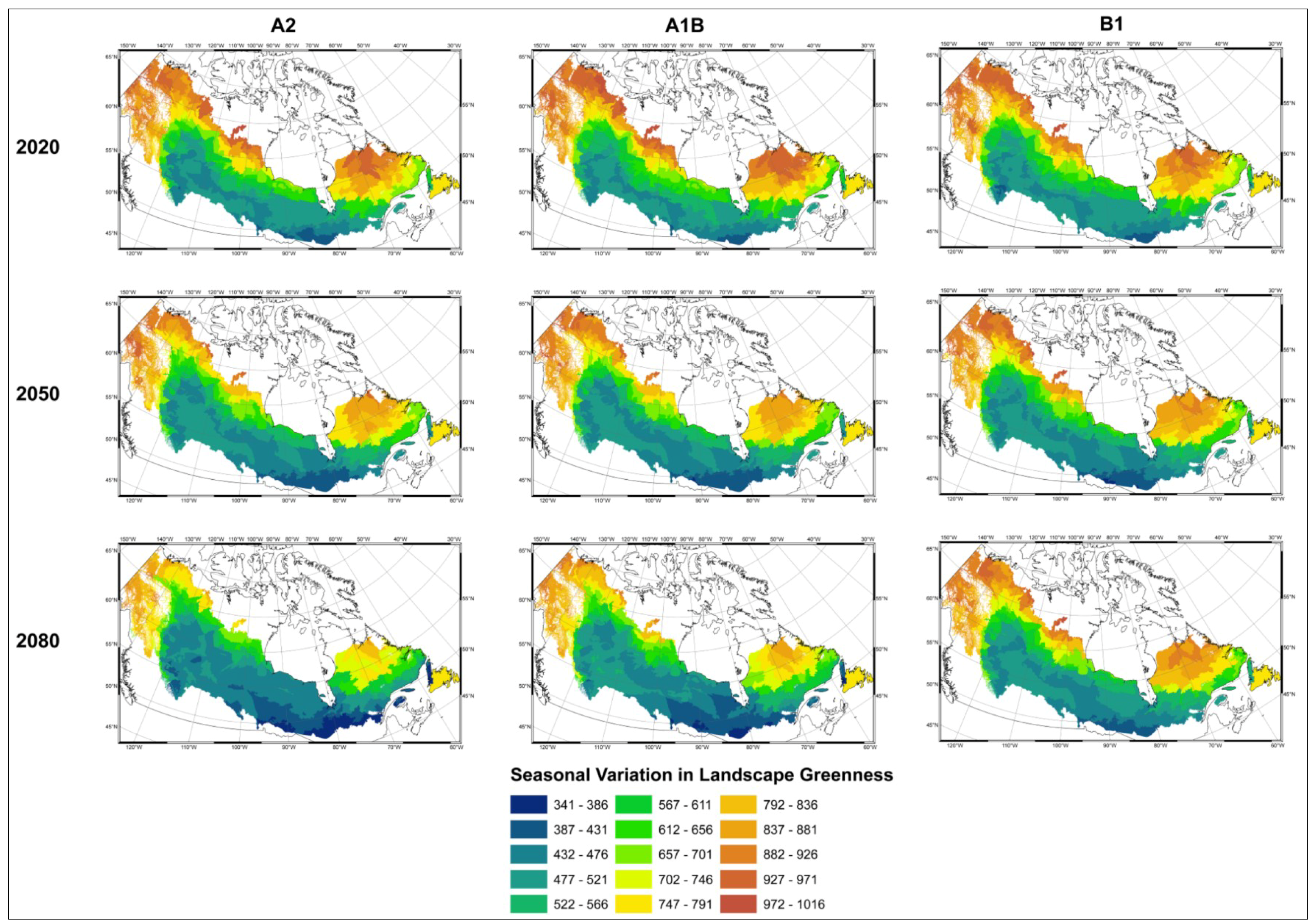
Modelled possible spatial distributions of vegetation productivity across Canada’s boreal in 2020, 2050, and 2080, using historical climate data, linked to historical remote sensing derived indirect indicators of vegetation productivity from 1987–2007, which are then projected using a range of future climate scenarios;

(2).

Assessed the performance of predictive models by comparing observed and predicted maps of vegetation productivity using a fuzzy map comparison approach, and

(3).

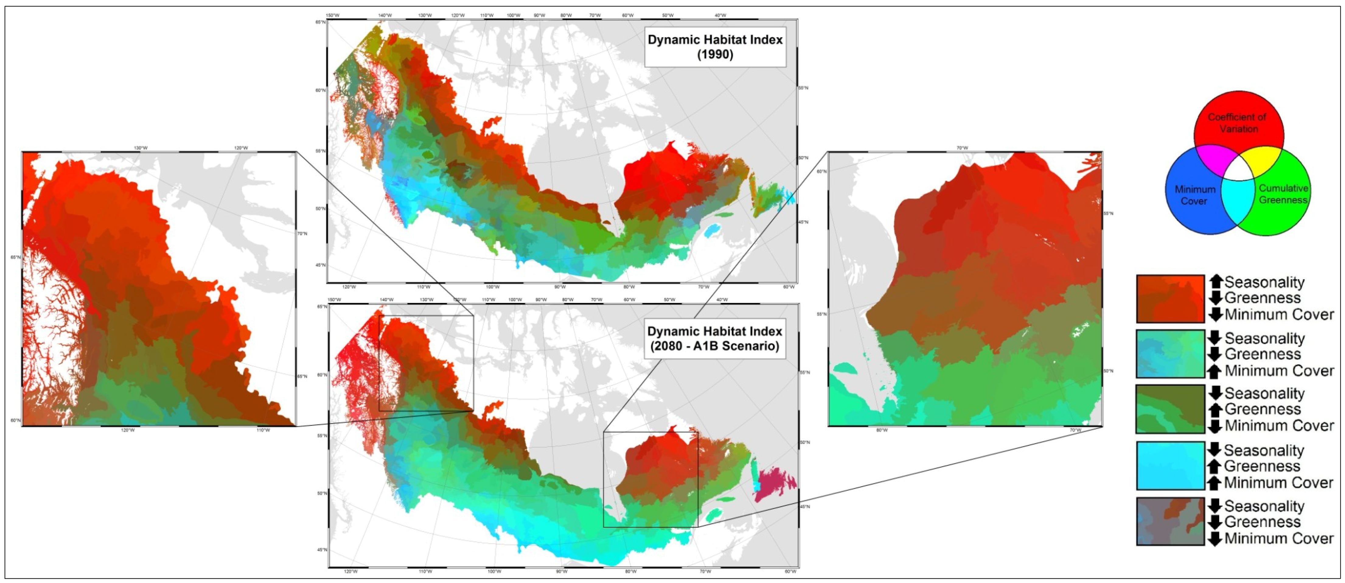
Mapped temporal variability in productivity predictions (from 2020, 2050, and 2080) to determine the locations where vegetation appears most and least sensitive to climate change.

2. Methods

2.1. Study Area and Data

The boreal region of Canada covers approximately 537 million km² and represents one quarter of all naturally functioning forests globally [41] (Figure 1). In contrast to the southern locations of the boreal zone where commercial forestry and human land uses are common, the northern boreal is shaped by active natural disturbances, principally fire [42,43,44]. Insect outbreaks are another important disturbance agent in Canada’s boreal [45]. Typically, insect outbreaks cause spatially localized disturbances. However, climate change is leading to unprecedented insect outbreaks that are having regional effects across North America [46,47]. The geographic distribution of productivity within the boreal forest is closely related to climatic regimes with the forests characterized by long, cold, dry winters and short, cool, moist summers.

Figure 1. Canadian boreal with ecozones.

Figure 1. Canadian boreal with ecozones.

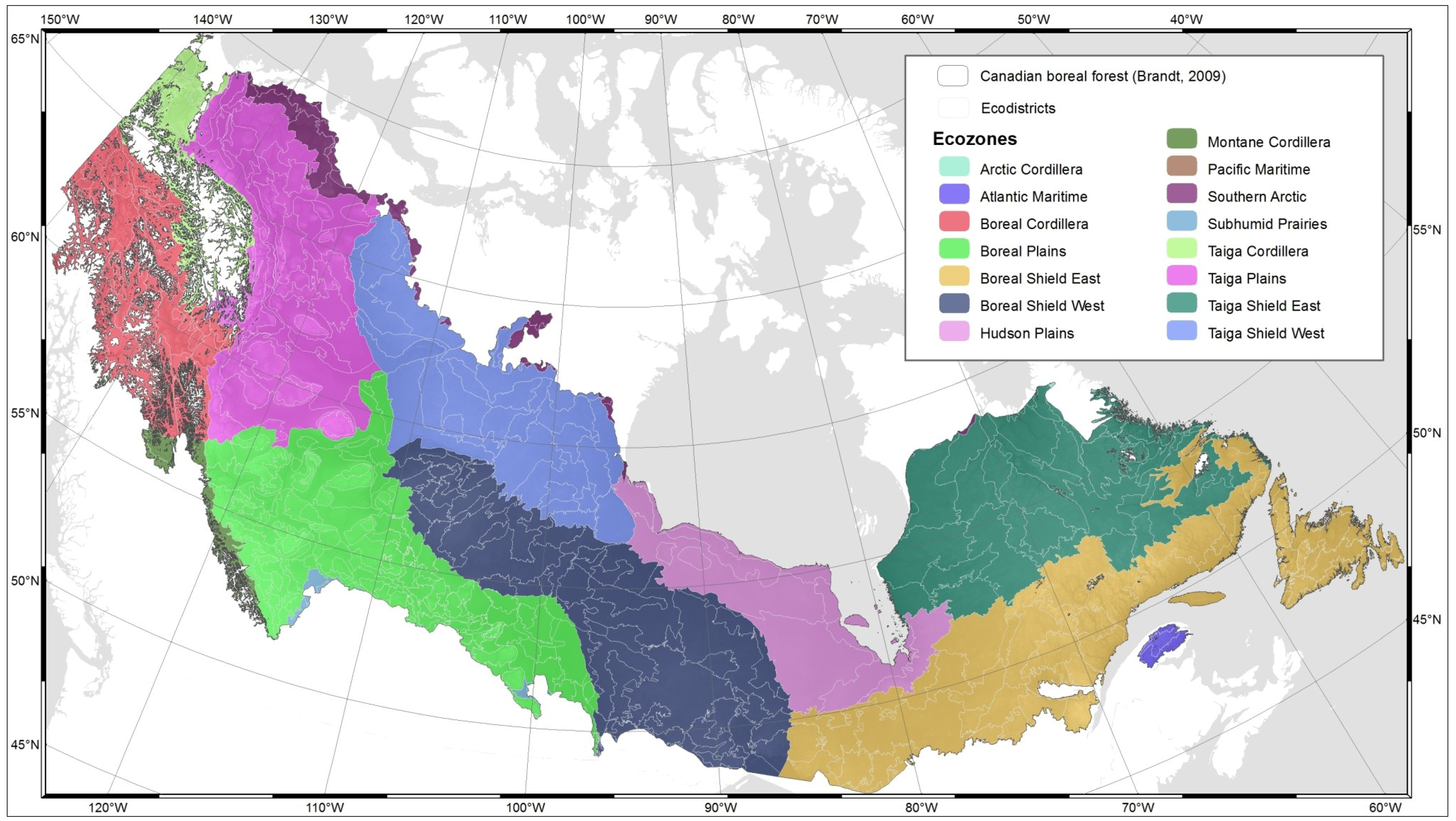
2.1.1. Ecodistricts and Ecozones

Due to the large spatial extent of the study area, ecozones and ecodistricts were used to provide geographic context and describe landscape characteristics. Ecozones and ecodistricts are two different landscape scales with homogenous and unique interactions between geologic, landform, soil, vegetation, climatic, water and human factors [48]. There are 15 ecoregions in Canada’s boreal (Table 1). The southern portion of the Boreal Plains ecozone is characterized by trembling aspen (Populous tremuloides) and balsam poplar (Populus balsamifera), as well as open parklands. The central portion of the boreal is covered largely by closed-canopy forest and is comprised of three distinct ecozones: the Boreal Plains, Boreal Shield, and Boreal Cordillera. In this research, as in others (e.g., [16,49]) the Boreal Shield and Taiga Shield are split into east and west units due to differences in precipitation and disturbance regimes. The northern boreal consists of sparse forest and open barrens extending to the northern limit of trees and is the least developed part of the Canadian boreal [15,50]. Within Canada’s boreal there are 592 ecodistricts with a minimum size of ~100 ha and these formed the basis of all mapping and predictions.

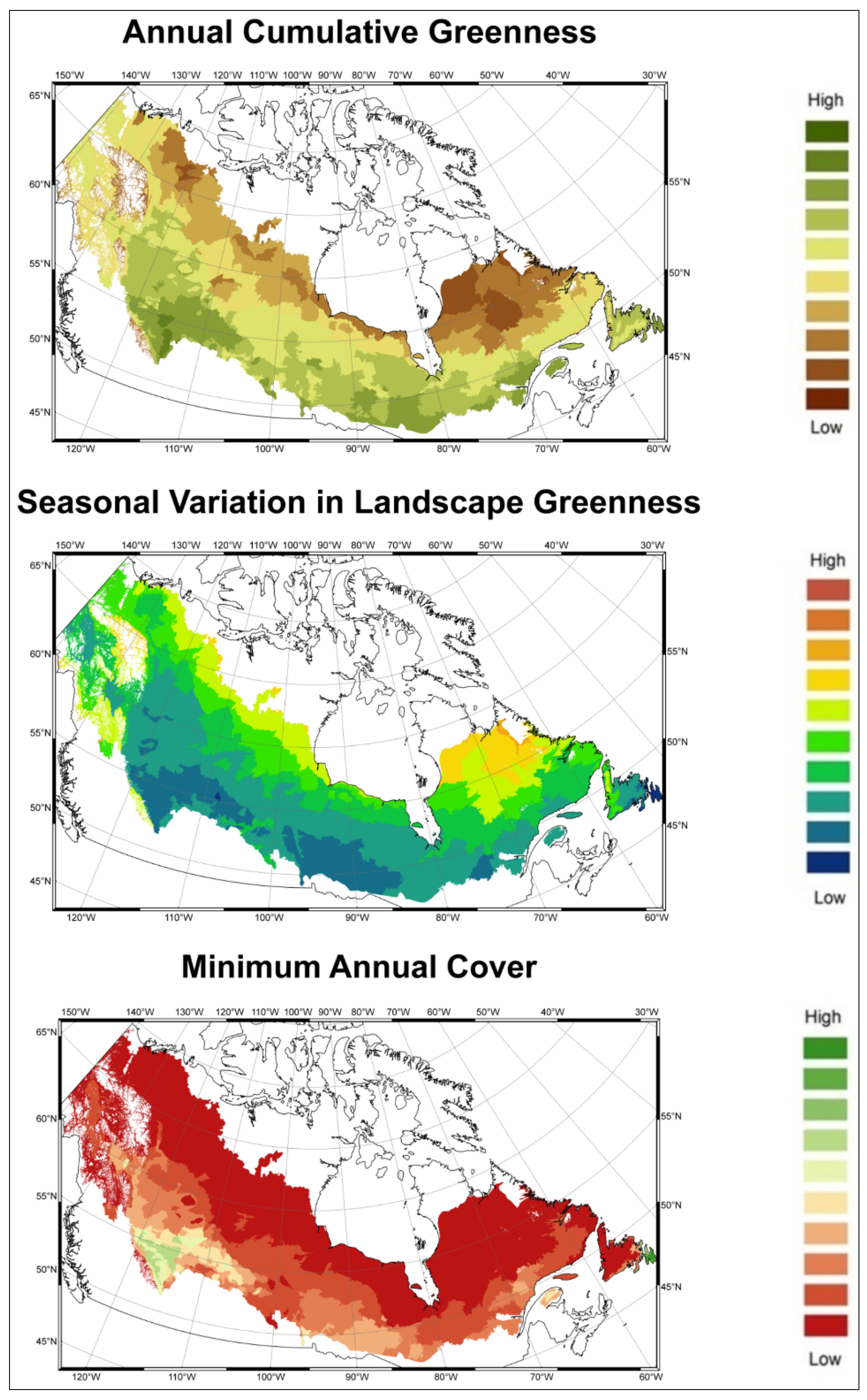
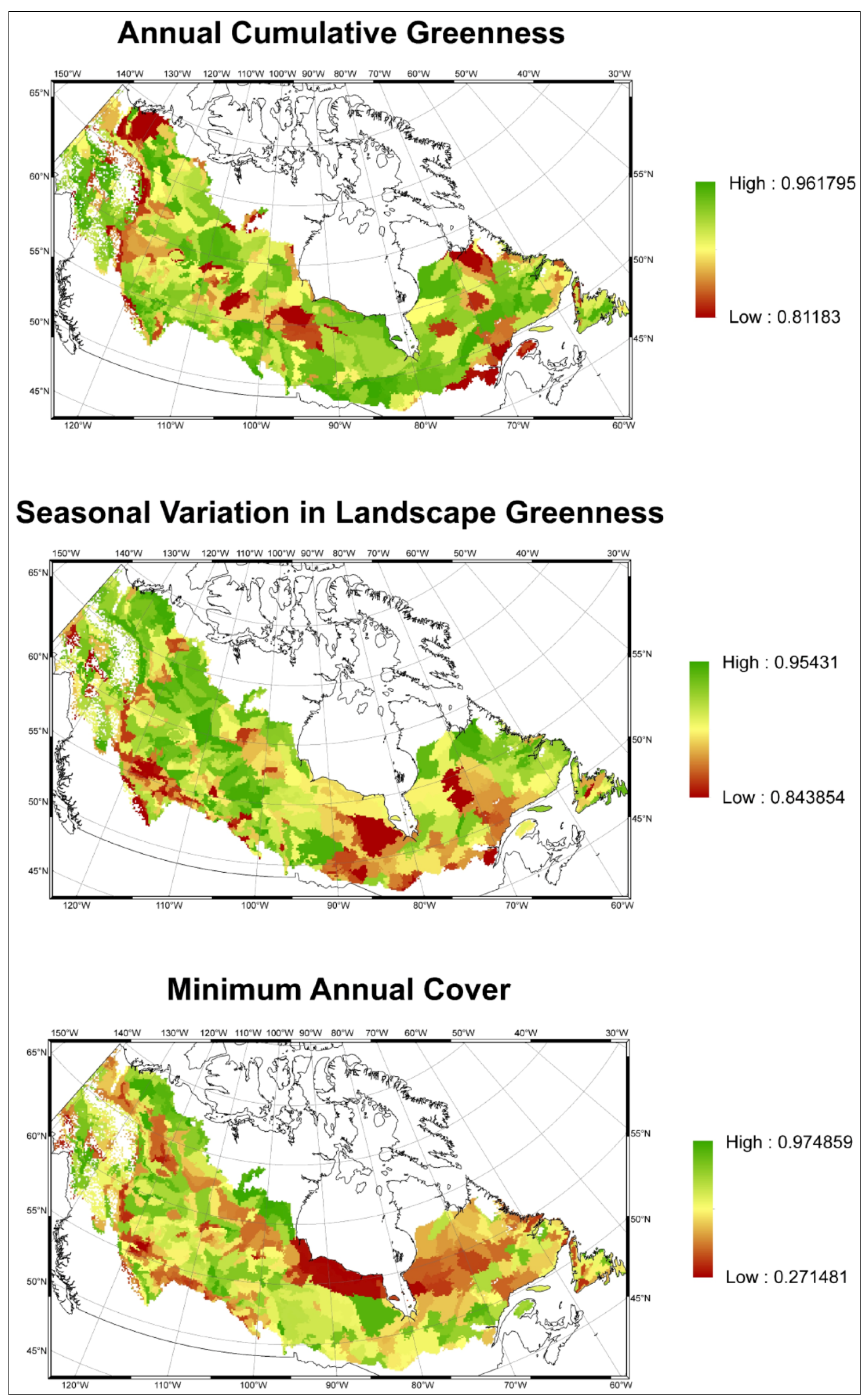
2.1.2. Indirect Biodiversity Indicators

The dynamic habitat index (DHI) is a representation of vegetation productivity and an indirect indicator of biodiversity. The DHI is acquired from three indices, calculated from monthly fPAR composite images, and derived from MODIS, MERIS or AVHRR reflectance values [5]. fPAR is a measure of the amount of radiation absorbed by the plant canopy during photosynthesis (400–700 nm wavelengths) [51]. A proxy for landscape vegetation primary productivity, fPAR is utilized as a surrogate measure for biodiversity [52]. For this research the DHI indices were computed from AVHRR data from 1987–2007 with a spatial resolution of 1 km [29], which is the only boreal-wide satellite dataset available over this time period. The three fPAR indices representing vegetation productivity that were combined into the DHI were: (i) annual cumulative greenness; (ii) seasonal variation in greenness; and (iii) minimum annual cover [5,38]. Annual cumulative greenness is an indication of overall vegetation productivity and the potential landscape productivity at any given location [19]. Annual cumulative greenness was estimated by summing monthly fPAR observations for each year [23]. Seasonal variation in greenness is directly related to local climate and geography and characterizes annual variations in vegetation productivity at a given location. Calculated as the coefficient of variation, seasonal variation in greenness is sensitive to extreme changes in vegetation cover such that the index is low in highly productive evergreen forests and high in areas exhibiting seasonal snow covers in the winter and vegetative growth in the spring. Minimum annual cover indicates the lowest amount of vegetated cover at a specific location within a year. Minimum annual cover provides information about the landscape’s capacity to support adequate levels of green vegetation cover and permanent resident species throughout the year [23]. Baseline data on annual cumulative greenness, seasonal variation in greenness, and minimum annual cover are provided in Figure 2. We set the baseline to 1990, as future predictions are provided at 30 year intervals for 2020, 2050, and 2080. The DHI in 1990 represents conditions 30 years prior to the first prediction and provides data at consistent time intervals.

Table 1. Ecozone descriptions for Canada’s boreal.

Ecozone	Landforms	Climate/ oceanographic characteristics	Vegetation/ productivity	Area (km2)
Arctic Cordillera	Mountains	Extremely cold, dry; continuous permafrost	Mainly unvegetated; some shrub-herb tundra	230,873
Atlantic Maritime	Hills and coastal plains	Cool, wet	Mixed deciduous-evergreen forest	183,978
Boreal Cordillera	Mountains, some hills	Moderately cold, moist	Largely evergreen forest; some tundra, open woodland	459,680
Boreal Plains	Plains, some foothills	Cold, moist	Mixed evergreen-deciduous forest	679,969
Boreal Shield East	Plains, some hills	Cold, moist	Evergreen forest, mixed evergreen, deciduous forest	1,782,252
Boreal Shield West
Hudson Plains	Plains	Cold to mild, semiarid; discontinuous permafrost	Wetland; some herb, lichen tundra, evergreen forest	353,364
Montane Cordillera	Mountains and interior plains	Moderately cold, moist to arid	Evergreen forest, alpine tundra, interior grassland	479,057
Pacific Maritime	Mountains, minor coastal plains	Mild, temperate, very wet to cold alpine	Coastal evergreen forest	205,175
Southern Arctic	Plains, hills	Cold, dry; continuous permafrost	Shrub-herb tundra	773,041
Subhumid Prairies	Plains, some hills	Cold, semiarid	Grass; scattered deciduous forest (“aspen parkland”)	469,681
Taiga Cordillera	Mountains	Cold, semiarid; discontinuous permafrost	Shrub-herb-moss-lichen tundra	264,480
Taiga Plains	Plains, some foothills	Cold, semiarid to moist; discontinous permafrost	Open to closed mixed evergreen-deciduous forest	580,139
Taiga Shield East	Plains, some hills	Cold, moist to semiarid; discontinuous permafrost	Open evergreen-deciduous trees; some lichen-shrub tundra	1,253,887
Taiga Shield West

Table 1. Ecozone descriptions for Canada’s boreal.

Ecozone	Landforms	Climate/ oceanographic characteristics	Vegetation/ productivity	Area (km2)
Arctic Cordillera	Mountains	Extremely cold, dry; continuous permafrost	Mainly unvegetated; some shrub-herb tundra	230,873
Atlantic Maritime	Hills and coastal plains	Cool, wet	Mixed deciduous-evergreen forest	183,978
Boreal Cordillera	Mountains, some hills	Moderately cold, moist	Largely evergreen forest; some tundra, open woodland	459,680
Boreal Plains	Plains, some foothills	Cold, moist	Mixed evergreen-deciduous forest	679,969
Boreal Shield East	Plains, some hills	Cold, moist	Evergreen forest, mixed evergreen, deciduous forest	1,782,252
Boreal Shield West
Hudson Plains	Plains	Cold to mild, semiarid; discontinuous permafrost	Wetland; some herb, lichen tundra, evergreen forest	353,364
Montane Cordillera	Mountains and interior plains	Moderately cold, moist to arid	Evergreen forest, alpine tundra, interior grassland	479,057
Pacific Maritime	Mountains, minor coastal plains	Mild, temperate, very wet to cold alpine	Coastal evergreen forest	205,175
Southern Arctic	Plains, hills	Cold, dry; continuous permafrost	Shrub-herb tundra	773,041
Subhumid Prairies	Plains, some hills	Cold, semiarid	Grass; scattered deciduous forest (“aspen parkland”)	469,681
Taiga Cordillera	Mountains	Cold, semiarid; discontinuous permafrost	Shrub-herb-moss-lichen tundra	264,480
Taiga Plains	Plains, some foothills	Cold, semiarid to moist; discontinous permafrost	Open to closed mixed evergreen-deciduous forest	580,139
Taiga Shield East	Plains, some hills	Cold, moist to semiarid; discontinuous permafrost	Open evergreen-deciduous trees; some lichen-shrub tundra	1,253,887
Taiga Shield West

Figure 2. The three fraction of photosynthetically active radiation (fPAR) indices that represent vegetation productivity and are combined to produce the dynamic habitat index (DHI): annual cumulative greenness; seasonal variation in greenness; and minimum annual cover. Annual cumulative greenness is an indication of overall vegetation productivity and the potential productivity at any given location. Seasonal variation in greenness is calculated as the coefficient of variation and is sensitive to extreme changes in vegetation cover. Minimum annual cover indicates the lowest amount of vegetated cover at a specific location within a year. Maps shown represent conditions in 1990.

Figure 2. The three fraction of photosynthetically active radiation (fPAR) indices that represent vegetation productivity and are combined to produce the dynamic habitat index (DHI): annual cumulative greenness; seasonal variation in greenness; and minimum annual cover. Annual cumulative greenness is an indication of overall vegetation productivity and the potential productivity at any given location. Seasonal variation in greenness is calculated as the coefficient of variation and is sensitive to extreme changes in vegetation cover. Minimum annual cover indicates the lowest amount of vegetated cover at a specific location within a year. Maps shown represent conditions in 1990.

2.1.3. Historical Climate Data

Historical climate data were provided by the Pacific Climate Impacts Consortium (PCIC) and were derived from models produced by the National Centers for Environmental Prediction (NCEP) North American Regional Reanalysis (NARR) project. The NARR project provides a long-term, dynamically consistent, high-resolution (32 km), high-frequency, atmospheric dataset for North America [53] that is available as point data. In order to spatially integrate the NARR data with the DHI, monthly climate datasets from 1987–2007 were interpolated using natural neighbours and stored in 1 km by 1 km grid cells. Daily climate variables were summarized annually and include precipitation (prec), maximum temperature (tmax), minimum temperature (tmin), and the mean annual growing season index (GSI) [54,55], which is an estimation of the mean vapour pressure deficit (iVDP) and mean suboptimal temperatures (iTmin). The vapour pressure deficit of the atmosphere serves as an index of vegetation evaporative demand where water stress constrains vegetation growth due to stomatal closure and reduced photosynthesis [6,54,56]. Suboptimal temperatures affect phenological development of vegetation during the first two to three months of the growing season, whereby cooler conditions retard and warmer conditions accelerate development [57]. The growing season index is computed by multiplying the suboptimal temperature, vapour pressure deficit, and photoperiod [54] and serves as indicator of the relative constraints to phenological development of vegetation due to climatic limits.

2.1.4. Scenarios of Future Climate

Three Intergovernmental Panel on Climate Change (IPCC) future climate scenarios were used: B1, A1B, and A2. The B1 scenario represents the least extreme climate change, the A1B (scenario represents business as usual, and the A2 represents the most extreme climate change. Based on the IPPC scenarios, maps of future climate for Canada’s boreal were obtained from the Canadian Centre for Climate Modelling and Analysis (CCCma) and represent the thirty-year climate averages centered on 2020, 2050, and 2080. By using three models we aimed to represent climate change conditions over a full range of possible scenarios [58]. Mote et al. [59] compared the ability of 10 global climate models to track recently recorded trends in temperature and precipitation in the Pacific northwest and reported that the Canadian model predicted trends consistent with other models, including a relatively rapid rate in warming and increases in precipitation when compared to actual observations.

2.2. Methods

2.2.1. Predicting Future Spatial Distributions of Forest Productivity

Described in more detail below, the general approach to prediction was to first quantify relationships between historical climate and the DHI. Using a Random Forest data mining technique that was used for each of the DHI components (annual cumulative greenness, seasonal variation in greenness, and minimum annual cover) we generated three 1987–2006 climate-productivity models. Using model fits, built from historical data, and future climate scenarios (A1B, A2, B1) each component of the DHI index was forecasted for the years 2020, 2050, and 2080, resulting in 27 future vegetation productivity maps at the spatial resolution of ecodistricts. In addition, the DHI indices were visualized in a composite image by simultaneously displaying seasonal variation in greenness, annual cumulative greenness, and minimum annual cover, which enabled interactions between the three DHI components to be explored.

For each of the three DHI components (annual cumulative greenness, seasonal variation in greenness, and minimum annual cover) a Random Forest model was generated to quantify relationships with historical climate data. Multiple fully grown regression trees (“the forest”) were used to create a model fit. These singular trees are formed by hierarchical binary partitions of singular predictor variables (ecoregion and climate indices) to explain the variation in the response variable (cumulative, seasonal and minimum fPAR levels) [60]. Predictor partitions were selected using iterative ANOVA analysis to ensure the greatest decrease in the sum of the squares within the vegetation productivity groups (see [61]). The variable selected at each split was chosen from a random subset of the predictors. Predictions of vegetation productivity at the terminal splits were averaged over all trees in the forest to predict the final annual productivity values [60]. In our case, 999 singular regression trees, created from boot-strapped samples, produced stable predictions.

The Random Forest algorithm was utilized for prediction as it does not make assumptions about the shapes of relationship and has been demonstrated to be a flexible model for ecological prediction [60,61]. Using an ensemble of trees is known to reduce error rates by smoothing the severity of the prediction boundaries created by singular regression trees [61]. In addition, the implementation of a second randomization step, of selecting a subset of predictors to be chosen from for the binary splits, is known to reduce the effects of redundant variables and allowed indices that may have been masked by dominant predictors to be selected [61,62]. The second randomization step also introduced a greater display of interaction effects between climate variables that may otherwise have been hidden [63].

Random Forest model fits for annual cumulative greenness, seasonal variation in greenness, and minimum annual cover, were assessed by the mean square error and percentage of variance explained, which is a generalized error rate calculated from out of the bag data [61], or data not used in the bootstrapped sample. To interpret which climate variable had the greatest influence on the productivity indices’ predictions, node purity was also used to indicate the average total reduced sum of the squares attained by all partitions on the environmental variable of interest [61].

2.2.2. Model Validation

For model validation the Random Forest models were applied to data from 1987–2006 to predict the three DHI indices in 2007. The 2007 observed and predicted maps of annual cumulative greenness, seasonal variation in greenness, and minimum annual cover were then compared using a technique known as fuzzy numerical map comparison [64]. The fuzzy numerical map comparison considers the similarity in modelled and observed values by quantifying how similar a DHI value is for a pixel, within the pixel’s spatial neighbourhood, and the mean of the map or study area. By comparison with the mean, the fuzzy numerical statistic identifies where the local pattern of similarity is unique [65]

(1)

S_i(A,B) = min(s_i(A,B),s_i(B,A))

(2)

(3)

(4)

Where s_i(A,B) is the one-way similarity between map A and B at cell i. Index j iterates through all N cells and the function w(d) defines the neighborhood, which defined by distance or, in this case, adjacent pixels. S_i(A,B) combines the two one-way similarities into an overall similarity. S(A,B) is the overall map similarity, it is the mean of overall n locations. The function f(a,b) determines the similarity of two values. The fuzzy numerical statistic values range from zero to one, where zero indicates no similarity and one indicates complete similarity.

3. Results

3.1. Predicting Future Spatial Distributions of Forest Productivity

For the annual cumulative greenness and seasonal variation in greenness, the models explained 79.3% and 79.0% of the variance respectively. Large increases in node purity and increases in mean square errors (after variable value permutations) indicated climate indices with the greatest importance to the overall prediction of annual vegetation productivity characteristics (Table 2). The variables with the strongest impact on node purity, a measure of the variable importance for cumulative vegetation production, were maximum temperature (tmax) and mean suboptimal temperatures (iTmin). Precipitation (prec) and mean vapour pressure deficit (iVDP) were the variables that when included reduced mean square error the most. For the minimum cover, the model explained 72.0% of variance and, as with the other models, maximum temperature (tmax) and mean suboptimal temperatures (iTmin) increased node purity. For minimum cover precipitation (prec) and mean annual growing season index (GSI) had the greatest impact on mean square error.

Table 2. Random Forest model fits. Percent increases in MSE (mean squared error) are indicative of the degree of the model fit based on the data used to train the Random Forest. Node purity is a summarized measure of how much the prediction was improved when the variable was selected (i.e., sum of the decrease in root mean square error across all trees in the forest).

DHI Indice	Annual Cumulative Greenness		Seasonal Variation in Greenness		Minimum Annual Cover
Variance Explained	79.33%		78.99%		71.98%
Measures of Variable Importance	% Increase MSE	Increases in Node Purity	% Increase MSE	Increases in Node Purity	% Increase MSE	Increases in Node Purity
Ecozone ID	74.12	5,169,808,231	74.44	19,389,848	37.81	1,824,596
prec	164.57	4,935,705,165	103.57	34,512,265	131.05	3,506,894
tmax	68.87	21,549,330,333	53.09	91,421,945	50.26	9,120,574
tmin	51.55	11,719,222,586	50.66	52,579,917	36.66	7,040,439
iVPD	101.22	4,630,608,283	78.10	38,235,056	77.19	34,769,256
iTmin	46.03	14,495,094,376	27.33	102,087,167	48.28	5,269,696
GSI	67.33	10,606,562,711	45.63	76,972,493	78.43	4,407,121

Table 2. Random Forest model fits. Percent increases in MSE (mean squared error) are indicative of the degree of the model fit based on the data used to train the Random Forest. Node purity is a summarized measure of how much the prediction was improved when the variable was selected (i.e., sum of the decrease in root mean square error across all trees in the forest).

DHI Indice	Annual Cumulative Greenness		Seasonal Variation in Greenness		Minimum Annual Cover
Variance Explained	79.33%		78.99%		71.98%
Measures of Variable Importance	% Increase MSE	Increases in Node Purity	% Increase MSE	Increases in Node Purity	% Increase MSE	Increases in Node Purity
Ecozone ID	74.12	5,169,808,231	74.44	19,389,848	37.81	1,824,596
prec	164.57	4,935,705,165	103.57	34,512,265	131.05	3,506,894
tmax	68.87	21,549,330,333	53.09	91,421,945	50.26	9,120,574
tmin	51.55	11,719,222,586	50.66	52,579,917	36.66	7,040,439
iVPD	101.22	4,630,608,283	78.10	38,235,056	77.19	34,769,256
iTmin	46.03	14,495,094,376	27.33	102,087,167	48.28	5,269,696
GSI	67.33	10,606,562,711	45.63	76,972,493	78.43	4,407,121

As models of climate change became more extreme, or as climate change continued through time, increased annual cumulative greenness shifts northward through Canada’s boreal and intensifies. The most extreme climate model scenario (A2) predicted the highest expansion of cumulative greenness into areas of the Hudson Plains wetlands and Taiga Plains tundra by 2080 (Figure 3). More conservative climate change scenarios, the A1B and B1 models, also predicted increased greenness, but the southern boreal forest was predicted to be more strongly impacted.

Figure 4 illustrates that as the climate changes, seasonal variation in greenness decreases. Future scenarios of seasonality indicated that the region around the Great Lakes is predicted, by the moderate (A1B) and high climate change (A2) scenarios, to be less seasonally coupled with an increase in cumulative productivity by 2080 (Figure 4). In contrast, the conservative climate change model (B1) indicated a reduction in the lowest seasonality class in the south boreal regions.

In general, minimum annual cover will decrease under increasing climate change. Forecasts showed a strong decrease in the southern portion of the Boreal Plains (Figure 5). However, throughout the Boreal Shield an increase in minimum cover was predicted, with the most extreme model (A2) predicted to have high minimum cover in the Hudson Plains’ region by 2080.

Simultaneous display of the three DHI indices for 1990 and the A1B scenario for 2080 allowed for more complex interpretation of habitat shifts due to the interaction of vegetation productivity processes (Figure 6). Results predicted reduced heterogeneity in vegetation productivity, particularly west of Hudson Bay as the complex colors shown in 1990 become more homogenous aqua and red in 2080. Reduced vegetation heterogeneity indicated that in the south, vegetation productivity is the expression of a combination of annual cumulative greenness and minimum annual cover, while in the north seasonal variation in greenness is the dominant process.

3.2. Model Validation

Comparison of the 2007 observed and predicted DHI generated fuzzy numerical values for the cumulative greenness ranging from 0.7–1.0 with a mean of 0.9 suggesting strong agreement. Fuzzy numerical values for the coefficient of variation or seasonality were similar, ranging from 0.6–1.0 with a mean of 0.9. The minimum cover had less agreement between observed and predicted with fuzzy numerical values ranging from 0.1–1.0 and a mean of 0.6.

The level of model agreement varied spatially (Figure 7). For annual cumulative greenness, the lowest agreement between modelled and observed 2007 data occurred primarily in the Southern Arctic and Taiga Plains and agreement was highest in the Hudson Plains. The Atlantic Maritime Ecozone, which is small in area, also showed poor agreement for annual cumulative greenness. For seasonal variation in greenness the lowest agreement occurred in the Hudson Plains, while the Taiga ecozones had the highest agreement. Minimum annual cover, overall, had much lower agreement, and the least agreement occurred in the Hudson Plains and Taiga Shield. All DHI indices had poor agreement in the Boreal Cordillera, likely due to the small area and thus the relationships that govern productivity may not be well represented in the model.

Figure 3. Predicted spatial distribution of annual cumulative greenness for 2020, 2050, and 2080 based on three Intergovernmental Panel on Climate Change (IPCC) climate change scenarios: A2 (most change), A1B (business as usual), and B1 (least change).

Figure 3. Predicted spatial distribution of annual cumulative greenness for 2020, 2050, and 2080 based on three Intergovernmental Panel on Climate Change (IPCC) climate change scenarios: A2 (most change), A1B (business as usual), and B1 (least change).

Figure 4. Predicted spatial distribution of seasonal variation in greenness for 2020, 2050, and 2080 based on three IPCC climate change scenarios: A2 (most change), A1B (business as usual), and B1 (least change).

Figure 4. Predicted spatial distribution of seasonal variation in greenness for 2020, 2050, and 2080 based on three IPCC climate change scenarios: A2 (most change), A1B (business as usual), and B1 (least change).

Figure 5. Predicted spatial distribution of minimum annual cover for 2020, 2050, and 2080 based on three IPCC climate change scenarios: A2 (most change), A1B (business as usual), and B1 (least change).

Figure 5. Predicted spatial distribution of minimum annual cover for 2020, 2050, and 2080 based on three IPCC climate change scenarios: A2 (most change), A1B (business as usual), and B1 (least change).

Figure 6. Composite DHI model results for observed 1990 and 2080 (A1B). Maps are a simultaneous display of the three DHI components where the red, green, and blue color bands represent seasonality, cumulative greenness, and minimum cover, respectively. Dark colored regions have low values in all DHI components while light colored areas have high values. Areas of definitive color indicate a dominant habitat indicator; for example a region that is purely red denotes high seasonal variation in greenness. As indicators shift in 2080, such as when seasonal variation in greenness decreases, other components such as annual cumulative greenness or minimum annual cover fill into newly favorable habitats. Common DHI blending occurred with light blue, yellow, and darker colorations like purple or dark orange. The light blue regions represent the most productive habitats with high minimum annual cover, high annual cumulative greenness, and low seasonal variation in greenness. Darker purple and orange colorations indicate low annual cumulative greenness, low seasonal variation in greenness, and low minimum annual cover.

Figure 6. Composite DHI model results for observed 1990 and 2080 (A1B). Maps are a simultaneous display of the three DHI components where the red, green, and blue color bands represent seasonality, cumulative greenness, and minimum cover, respectively. Dark colored regions have low values in all DHI components while light colored areas have high values. Areas of definitive color indicate a dominant habitat indicator; for example a region that is purely red denotes high seasonal variation in greenness. As indicators shift in 2080, such as when seasonal variation in greenness decreases, other components such as annual cumulative greenness or minimum annual cover fill into newly favorable habitats. Common DHI blending occurred with light blue, yellow, and darker colorations like purple or dark orange. The light blue regions represent the most productive habitats with high minimum annual cover, high annual cumulative greenness, and low seasonal variation in greenness. Darker purple and orange colorations indicate low annual cumulative greenness, low seasonal variation in greenness, and low minimum annual cover.

Figure 7. Map comparison results comparing modelled and observed DHI components in 2007. Values are an average of map comparison values for each ecozone, where high values indicate more similarity between observed and modelled maps.

Figure 7. Map comparison results comparing modelled and observed DHI components in 2007. Values are an average of map comparison values for each ecozone, where high values indicate more similarity between observed and modelled maps.

4. Discussion

Developing climate/vegetation relationships from 1987 to 2006 and then predicting 2007 vegetation spatial distributions (as DHI indices) allowed assessment of model performance beyond variance explained. Both model variance explained and model performance were quite high, 72.0%–74.0% and a mean of 0.6–0.9 respectively. Though, minimum annual cover model performance was highly variable and as low as 0.1. High variability in predictive success of minimum annual cover may be related to low variance, as minimum annual cover could be low for several different environments [39]. For example, minimum annual cover will be low in deciduous forests as well as grasslands. Given the large spatial extent of our study area it was essential that the interaction between climate processes and vegetation vary geographically. By building a spatially explicit model that included ecozones, we did not assume spatial non-stationarity. Rather, we allowed modelled relationships between climate and vegetation to be developed based on regional dynamics [61].

Using geographically explicit map comparison, we were also able to quantify the geographic nature of uncertainty and better understand ecological factors influencing model confidence [66]. Annual cumulative greenness was typically low in areas with long winters and cool summers (Southern Arctic and Taiga Plains), possibly reflecting the importance of temperature in the model (Figure 3). The Atlantic Maritime Ecozone, which also showed poor agreement, may be impacted by oceanic influence that mediates climate [3] and reduced associations between temperature and vegetation productivity [67,68]. The lower agreement between modelled and predicted results for seasonal variation in greenness in the Hudson Plains may reflect the presence of the largest contiguous wetland in the world [26,69]. Wetlands are a complex mosaic of vegetation (trees, shrubs, and herbs) interspersed with water bodies of various sizes, posing a difficult environment for consistent capture with coarse spatial resolution remote sensing [26,70]. Much of the vegetation in the Hudson Plains is low and easily covered with temporally dynamic snow and ice [5]. In contrast to forest dominated environments, wetlands express cover and seasonality characteristics that are not as well captured using the remote sensing methods, with further investigation warranted. Minimum annual cover produced much lower levels of agreement between observed and modelled maps and was more difficult to model due to numerous near zero values, which can occur in environments ranging from rock and ice to locations exhibiting vegetation senescence cycles. The lowest agreement occurred in the Hudson Plains, which again could be the result of the unique response of wetlands [5,26,70,71], and in the Taiga Shield, where a patchwork of wetlands, forests, meadows, and shrub occurs in a cold climate [69]. The strength of mapping minimum annual cover is best realized when it is utilized in conjunction with annual cumulative greenness.

Maps of modelled change in individual DHI indices indicated that overall cumulative greenness will increase, seasonality will decrease, and minimum cover will increase. Similar trends have been predicted for other regions of Canada [39]. The amount of change will vary spatially and increase through time with more extreme climate scenarios (Figure 3, Figure 4 and Figure 5). A north/south gradient of change was apparent and matches the observed and experienced temperature increases north of 40° latitude [1]. These mid to high latitudes have had diurnal decreases in temperature ranges and decadal increases in autumn and winter precipitation contributing already to a 10% decrease in snow cover and ice extent exacerbated in the most northern extents [72]. Using the composite image we can identify, using the legend, how the combination of DHI components are expressed spatially. The composite images of DHI from 1990 and 2080 (Figure 6) revealed that, when compared to 1990, vegetation productivity modelled to 2080 (using the business-as-usual (A1B) climate change scenario) will be most impacted by the increased seasonality predicted in the north and a combination of cumulative greenness and minimum cover in the south. More inter- and intra-annual variability in precipitation and snowfall is expected [73]. Areas in the west and east were modelled as changing the most. For example, Newfoundland is currently influenced by multiple productivity components and predicted to be strongly impacted by a combination of seasonality and minimum cover with a reduction in cumulative greenness. In the northwest, the Boreal Cordillera, Taiga Cordillera, and western portion of the Taiga Plains will also undergo substantive change influenced by seasonality more than any other DHI indices.

The relatively large predicted change in vegetation in the Hudson Plains and associated wetlands (Figure 3, Figure 4, Figure 5 and Figure 6) is in line with other research that has indicated climate change is a major threat to the integrity of wetlands [74]. Relative to other wetlands worldwide, the high latitude of Canada’s wetlands make them particularly vulnerable to climate change [75]. Previous research has suggested that drier and warmer conditions may lead to a 70%–90% loss of wetlands in the Hudson Plains [76]. Reduced duration of snow cover, associated with predicted increases in minimum greenness and decreased seasonality, will negatively impact some duck species in boreal wetlands [77]. For example, reduced flexibility in timing of breeding has been predicted to impact population levels of species such as scaups (Aythya spp.) and scoters (Melanitta spp.).

The Taiga has similar climate characteristics but different geology, flora, and fauna [71] to the Hudson Plains and was predicted to undergo substantial change in vegetation (west for annual cumulative greenness; east for seasonal variation in greenness and minimum annual cover). The Taiga is characterized by discontinuous permafrost and annual temperatures that are below freezing. Observing rapid change the Taiga may indicate that climate change will surpass a threshold that will cause a substantive response in vegetation [78]. For instance, in the western Taiga, Olthof and Pouliot [78] predicted conifer recruitment and growth would occur in the north.

A striking result of the composite images was the loss of heterogeneity in the DHI. Increased homogeneity may lead to reductions in species richness with fewer niches for species to select [79]. Examples of species of particular concern is the yellow rail (Coturnicops noveboracensis), an at-risk wetland bird whose narrow breeding habitat and important boreal breeding ranges south of Hudson and James Bay lowlands makes it especially vulnerable. Yellow rail breeding habitat is tightly constrained to shallow water levels (i.e., <15 cm for initial nesting) and the availability of overlying dry dead mats of vegetation, environments akin to wet marshy areas dominated by grass-like vegetation [80]. As such, climate-induced habitat loss or degradation through wetland reduction or shifts in wetland configuration and altered hydrological conditions, such as flooding or drought, represent an important threat to this species [80].

Research has previously documented that wide-ranging and sensitive species, such as birds and butterflies, follow vegetation productivity trends modelled by remotely sensed imagery [20,21,22,23,27,28,81]. Notably, seasonal trends captured by the fPAR index have been able to distinguish spatial variation in bird species richness, including species’ responses to seasonal and minimum annual productivity levels [23] and associations between composite DHI heterogeneity [81]. Demonstrated associations between vegetation productivity, represented by fPAR and the DHI index, suggest that predicting future possible spatial distributions of vegetation productivity provides guidance on how species spatial distributions may change. The strength of our approach is that it is general, covers a large area, and is repeatable. We provide a landscape perspective on predicted trends in the response of vegetation to climate change. The response of vegetation to climate is anticipated to correlate with change in species richness and distributions. However, responses will be complex and impacted by the interaction between multiple species [2] and nonlinear responses of species to climate change [82]. Our results are most appropriately interpreted as broad scale and relatively trends on spatial variation in the response of vegetation productivity and species distribution to climate change [9].

While our projections showed that climate change may increase the overall potential for greenness, other factors were not accounted for. For instance, soils will not change at the same rate as climate and may become a stronger limiting factor for vegetation growth. For example, our models showed potential increased greenness in higher elevations but thin soils may limit vegetation development. As well our models do not capture episodic events and climate extremes, such as droughts and flooding [72] or forest fire [43], which are all expected to increase in either magnitude or frequency due to climate change [83].

5. Conclusions

We have integrated historical climate and vegetation productivity data with future IPCC scenarios of climate change to map future spatial distributions of indirect indicators of biodiversity for Canada’s boreal. Our results indicate that vegetation productivity, an indirect indicator of biodiversity, will become more homogenous, particularly west of Hudson Bay. We can also expect climate to impact biodiversity along north/south gradients and by 2080 vegetation distributions will be dominated by processes of seasonal variation in greenness in the north and a combination of annual cumulative greenness and minimum annual cover in the south. The Hudson Plains are modelled as having the potential to experience substantive change becoming more productive or green with less seasonality.

In this research, we highlighted opportunities for space-time modelling of indirect indicators of biodiversity. Remote sensing provides datasets with continuous spatial coverage and long temporal extents and these are beneficial for mapping and modelling how vegetation has and will change. Though all models suffer uncertainty, managers tasked with planning and conserving biodiversity, particularly in large areas like Canada’s boreal, benefit from information on possible trends and changes in vegetation. The maps generated thorough this research are not the final word. One of the strengths of our methodology is that models and maps can be updated as new and better data come online. However, representations of future trends in vegetation productivity provide important context for long-term decision making and possible adaptation opportunities in Canada’s boreal.

References and Notes

1. Serreze, M.C.; Walsh, J.E.; Chapin, F.S., III; Osterkamp, T.; Dyurgerov, M.; Romanovsky, V.; Oechel, W.C.; Morison, J.; Zhang, T.; Barry, R.G. Observational evidence of recent change in the northern high-latitude environment. Clim. Change 2000, 46, 159–207. [Google Scholar] [CrossRef]
2. Walther, G.-R.; Post, E.; Convey, P.; Menzel, A.; Parmesan, C.; Beebee, T.J.C.; Fromentin, J.-M.; Hoegh-Guldberg, O.; Bairlein, F. Ecological responses to recent climate change. Nature 2002, 416, 389–395. [Google Scholar] [CrossRef]
3. Hamann, A.; Wang, T. Potential effects of climate change on ecosystem and tree species distribution in British Columbia. Ecology 2006, 87, 2773–2786. [Google Scholar] [CrossRef]
4. Nemani, R.R.; Keeling, C.D.; Hashimoto, H.; Jolly, W.M.; Piper, S.C.; Tucker, C.J.; Myneni, R.B.; Running, S.W. Climate-driven increases in global terrestrial net primary production from 1982 to 1999. Science 2003, 300, 1560–1563. [Google Scholar] [CrossRef]
5. Coops, N.C.; Wulder, M.A.; Duro, D.; Han, T.; Berry, S. The development of a Canadian dynamic habitat index using multi-temporal satellite estimates of canopy light absorbance. Ecol. Indic. 2008, 8, 754–766. [Google Scholar] [CrossRef]
6. Weiss, J.L.; Castro, C.L.; Overpeck, J.T. Distinguishing pronounced droughts in the southwestern United States: Seasonality and effects of warmer temperatures. J. Clim. 2009, 22, 5918–5932. [Google Scholar] [CrossRef]
7. Rinawati, F.; Stein, K.; Lindner, A. Climate change impacts on biodiversity—the setting of a lingering global crisis. Diversity 2013, 5, 114–123. [Google Scholar] [CrossRef]
8. Soja, A.; Tchebakova, N.; French, N.; Flannigan, M.; Shugart, H.; Stocks, B.; Sukhinin, A.; Parfenova, E.; Chapin, F.; Stackhouse, P., Jr. Climate-induced boreal forest change: Predictions versus current observations. Global Planet. Change 2007, 56, 274–296. [Google Scholar] [CrossRef]
9. Volney, W.J.A.; Fleming, R.A. Climate change and impacts of boreal forest insects. Agr. Ecosyst. Environ. 2000, 82, 283–294. [Google Scholar] [CrossRef]
10. Wulder, M.A.; White, J.C.; Han, T.; Coops, N.C.; Cardille, J.A.; Holland, T.; Grills, D. Monitoring Canada’s forests. Part 2: National forest fragmentation and pattern. Can. J. Rem. Sens. 2008, 34, 563–584. [Google Scholar] [CrossRef]
11. Geider, R.J.; Delucia, E.H.; Falkowski, P.G.; Finzi, A.C.; Grime, J.P.; Grace, J.; Kana, T.; la Roche, J.; Long, S.P.; Osborne, B.A.; et al. Primary productivity of planet earth: Biological determinants and physical constraints in terrestrial and aquatic habitats. Global Change Biol. 2001, 7, 849–882. [Google Scholar] [CrossRef]
12. Soulé, M.E.; Estes, J.A.; Miller, B.; Honnold, D.L. Strongly interacting species: Conservation policy, management, and ethics. Bioscience 2005, 55, 168–176. [Google Scholar] [CrossRef]
13. Bradshaw, W.E.; Holzapfel, C.M. Evolutionary response to rapid climate change. Science 2006, 312, 1477–1478. [Google Scholar] [CrossRef]
14. Smith, W.; Lee, P. Canada’s Forests at a Crossroads: An Assessment in the Year 2000; World Resources Institute: Washington, DC, USA, 2000. [Google Scholar]
15. Andrew, M.E.; Wulder, M.A.; Coops, N.C. Identification of de facto protected areas in boreal Canada. Biol. Conserv. 2012, 146, 97–107. [Google Scholar] [CrossRef]
16. Bolton, D.K.; Coops, N.C.; Wulder, M.A. Measuring forest structure along productivity gradients in the Canadian boreal with small-footprint Lidar. Environ. Monitor. Assess. 2013, 185, 6617–6634. [Google Scholar] [CrossRef]
17. Tilman, D.; Hill, J.; Lehman, C. Carbon-negative biofuels from low-input high-diversity grassland biomass. Science 2006, 314, 1598–1600. [Google Scholar] [CrossRef]
18. Wright, D.H. Species-energy theory: An extension of species-area theory. Oikos 1983, 41, 496–506. [Google Scholar] [CrossRef]
19. Berry, S.; MacKey, B.; Brown, T. Potential applications of remotely sensed vegetation greenness to habitat analysis and the conservation of dispersive fauna. Pac. Conserv. Biol. 2007, 13, 120–127. [Google Scholar]
20. Hurlbert, A.H.; Haskell, J.P. The effect of energy and seasonality on avian species richness and community composition. Am Nat. 2003, 161, 83–97. [Google Scholar] [CrossRef]
21. Hawkins, B.A. Summer vegetation, deglaciation and the anomalous bird diversity gradient in eastern North America. Global Ecol. Biogeogr. 2004, 13, 321–325. [Google Scholar] [CrossRef]
22. Evans, K.L.; Neil, J.A.; Kevin, J. Abundance, species richness and energy availability in the North American avifauna. Global Ecol. Biogeogr. 2006, 15, 365–378. [Google Scholar]
23. Coops, N.C.; Waring, R.H.; Wulder, M.A.; Pidgeon, A.M.; Radeloff, V.C. Bird diversity: A predictable function of satellite-derived estimates of seasonal variation in canopy light absorbance across the United States. J. Biogeogr. 2009, 36, 905–918. [Google Scholar] [CrossRef]
24. Fitterer, J.L.; Nelson, T.A.; Coops, N.C.; Wulder, M.A. Modelling the ecosystem indicators of British Columbia using Earth observation data and terrain indices. Ecol. Indic. 2012, 20, 151–162. [Google Scholar] [CrossRef]
25. Ivits, E.; Cherlet, M.; Horion, S.; Fensholt, R. Global biogeographical pattern of ecosystem functional types derived from Earth observation data. Rem. Sens. 2013, 5, 3305–3330. [Google Scholar] [CrossRef]
26. Powers, R.P.; Coops, N.C.; Morgan, J.L.; Wulder, M.A.; Nelson, T.A.; Drever, C.R.; Cumming, S.G. A remote sensing approach to biodiversity assessment and regionalization of the Canadian boreal forest. Prog. Phys. Geog. 2013, 37, 36–62. [Google Scholar] [CrossRef]
27. Fitterer, J.L.; Nelson, T.A.; Coops, N.C.; Wulder, M.A.; Mahony, N. Exploring the ecological processes driving geographical patterns of breeding bird richness in British Columbia Canada. Ecol. Appl. 2013, 23, 888–903. [Google Scholar] [CrossRef]
28. Andrew, M.E.; Wulder, M.A.; Coops, N.C. Patterns of protection and threats along productivity gradients in Canada. Biol. Conserv. 2011, 144, 2891–2901. [Google Scholar] [CrossRef]
29. Fontana, F.M.; Coops, N.C.; Khlopenkov, K.V.; Trishchenko, A.P.; Riffler, M.; Wulder, M.A. Generation of a novel 1 km NDVI data set over Canada, the northern United States, and Greenland based on historical AVHRR data. Rem. Sens. Environ. 2012, 121, 171–185. [Google Scholar] [CrossRef]
30. Hawkins, B.A.; Field, R.; Cornell, H.V.; Currie, D.J.; Guégan, J.F.; Kaufman, D.M.; Kerr, J.T.; Mittelbach, G.G.; Oberdorff, T.; O’Brien, E.M.; et al. Energy, water, and broad-scale geographic patterns of species richness. Ecology 2003, 84, 3105–3117. [Google Scholar] [CrossRef]
31. Field, R.; Hawkins, B.A.; Cornell, H.V.; Currie, D.J.; Diniz-Filho, J.A.F.; Guégan, J.-F.; Kaufman, D.M.; Kerr, J.T.; Mittelbach, G.G.; Oberdorff, T.; et al. Spatial species-richness gradients across scales: A meta-analysis. J. Biogeogr. 2009, 36, 132–147. [Google Scholar] [CrossRef]
32. Dallmeier, F.; Comiskey, J. (Eds.) Forest Biodiversity Research, Monitoring and Modeling: Conceptual Background and Old World Case Studies; The Parthenon Publishing Group: Pearl River, NY, USA, 1998.
33. Chase, J.M.; Leibold, M.A. Spatial scale dictates the productivity-biodiversity relationship. Nature 2002, 416, 427–430. [Google Scholar] [CrossRef]
34. Kerr, J.T.; Southwood, T.R.; Cihlar, J. Remotely sensed habitat diversity predicts butterfly species richness and community similarity in Canada. Proc. Nat. Acad. Sci. USA. 2001, 98, 11365–11370. [Google Scholar] [CrossRef]
35. Nagendra, H. Using remote sensing to assess biodiversity. Int. J. Remote Sens. 2001, 22, 2377–2400. [Google Scholar] [CrossRef]
36. Turner, W.; Spector, S.; Gardiner, N.; Fledeland, M.; Sterling, E.; Steininger, M. Remote sensing for biodiversity science and conservation. Trends Ecol. Evol. 2003, 18, 306–314. [Google Scholar] [CrossRef]
37. Nilsen, E.B.; Herfindal, I.; Linnell, J.D.C. Can intra-specific variation in carnivore home-range size be explained using remote-sensing estimates of environmental productivity? Ecoscience 2005, 12, 68–75. [Google Scholar] [CrossRef]
38. Duro, D.; Coops, N.C.; Wulder, M.A.; Han, T. Development of a large area biodiversity monitoring system driven by remote sensing. Progr. Phys. Geogr. 2007, 31, 235–260. [Google Scholar] [CrossRef]
39. Holmes, K.; Nelson, T.; Coops, N.C.; Wulder, M.A. Biodiversity indicators show climate change will alter vegetation in parks and protected areas. Diversity 2013, 5, 352–373. [Google Scholar] [CrossRef]
40. Kurz, W.A.; Stinson, G.; Rampley, G. Could increased boreal forest ecosystem productivity offset carbon losses from increased disturbances? Philos. T. R. Soc. B 2008, 363, 2259–2268. [Google Scholar] [CrossRef]
41. Brandt, J.P. The extent of the North American boreal zone. Environ. Rev. 2009, 17, 101–161. [Google Scholar] [CrossRef]
42. Amiro, B.D.; Cantin, A.; Flannigan, M.D.; de Groot, W.J. Future emissions from Canadian boreal forest fires. Can. J. Forest Res. 2009, 39, 383–395. [Google Scholar] [CrossRef]
43. Gralewicz, N.J.; Nelson, T.A.; Wulder, M.A. Factors influencing national scale wildfire susceptibility in Canada. Forest Ecol. Manage. 2012, 265, 20–29. [Google Scholar] [CrossRef]
44. Gralewicz, N.J.; Nelson, T.A.; Wulder, M.A. Spatial and temporal patterns of wildfire ignitions in Canada from 1980 to 2006. Int. J. Wildl. Fire 2012, 21, 230–242. [Google Scholar] [CrossRef]
45. Bergeron, Y.; Fenton, N.J. Boreal forests of eastern Canada revisited: Old growth, nonfire disturbances, forest succession, and biodiversity. Botany 2012, 90, 509–523. [Google Scholar] [CrossRef]
46. Robertson, C.; Farmer, C.J.; Nelson, T.A.; Mackenzie, I.; Wulder, M.A.; White, J.C. Determination of the compositional change (1999–2006) in the pine forests of British Columbia due to mountain pine beetle infestation. Environ. Monitor. Assess. 2009, 158, 593–608. [Google Scholar] [CrossRef]
47. Robertson, C.; Nelson, T.A.; Jelinski, D.E.; Wulder, M.A.; Boots, B. Spatial-temporal analysis of species’ range expansion: the case of the mountain pine beetle, Dendroctonus ponderosae. J. Biogeogr. 2009, 36, 1446–1458. [Google Scholar] [CrossRef]
48. Rowe, J.S.; Sheard, J.W. Ecological land classification: a survey approach. Environ. Manage. 1981, 5, 451–464. [Google Scholar] [CrossRef]
49. Stinson, G.; Kurz, W.A.; Smyth, C.E.; Neilson, E.T.; Dymond, C.C.; Metsaranta, J.M.; Blain, D. An inventory-based analysis of Canada’s managed forest carbon dynamics, 1990 to 2008. Global Change Biol. 2011, 17, 2227–2244. [Google Scholar] [CrossRef]
50. NRTEE (National Round Table on the Environment and the Economy). Boreal Futures: Governance, Conservation and Development in Canada’s Boreal; Renouf Publishing Company Ltd.: Ottawa, Canada, 2005. Available online: http://www.stakeholderforum.org/fileadmin/files/boreal-futures-eng.pdf (accessed on 21 February 2013).
51. Asrar, G.; Fuchs, M.; Kanemasu, E.T.; Hatfield, J.L. Estimating absorbed photosynthetic radiation and leaf area index from spectral reflectance in wheat. Agron. J. 1984, 76, 300–306. [Google Scholar] [CrossRef]
52. Xiao, J.; Moody, A. Geographical distribution of global greening trends and their climatic correlates: 1982–1998. Int. J. Remote Sens. 2005, 26, 2371–2390. [Google Scholar] [CrossRef]
53. Mesinger, F.; DiMego, G.; Kalnay, E.; Mitchell, K.; Shafran, P.C.; Ebisuzaki, W.; Jović, D.; Woollen, J.; Rogers, E.; Berbery, E.H.; et al. North American regional reanalysis. Bull. Am. Meteorol. Soc. 2006, 87, 343–360. [Google Scholar] [CrossRef]
54. Jolly, W.M.; Nemani, R.; Running, S.W. A generalized, bioclimatic index to predict foliar phenology in response to climate. Global Change Biol. 2005, 11, 619–632. [Google Scholar] [CrossRef]
55. Stöckli, R.; Rutishauser, T.; Baker, I.; Liniger, M.A.; Denning, A.S. A global reanalysis of vegetation phenology. J. Geophys. Res. 2011, 116, 1–19. [Google Scholar]
56. Salah, H.B.H.; Tardieu, F. Quantitative analysis of the combined effects of temperature, evaporative demand and light on leaf elongation rate in well-watered field and laboratory-grown maize plants. J. Exp. Bot. 1996, 47, 1689–1698. [Google Scholar] [CrossRef]
57. Cleary, B.D.; Waring, R.H. Temperature: Collection of data and its analysis for the interpretation of plant growth and distribution. Can. J. Bot. 1969, 47, 167–173. [Google Scholar] [CrossRef]
58. Murdock, T.Q.; Spittlehouse, D.L. Selecting and Using Climate Change Scenarios for British Columbia; Pacific Climate Impacts Consortium: Victoria, BC, Canada, 2011; p. 39. [Google Scholar]
59. Mote, P.; Salathé, E.; Peacock, C. Scenarios of Future Climate for the Pacific Northwest. Available online: http://cses.washington.edu/db/pdf/kc05scenarios462.pdf (Accessed on 21 February 2014).
60. Breiman, L.E.O. Random forests. Machine Learn. 2001, 45, 5–32. [Google Scholar] [CrossRef]
61. Prasad, A.; Iverson, L.; Liaw, A. Newer classification and regression tree techniques: Bagging and random forests for ecological prediction. Ecosystems 2006, 9, 181–199. [Google Scholar] [CrossRef]
62. Archer, K.J.; Kimes, R.V. Empirical characterization of random forest variable importance measures. Computation. Stat. Data Anal. 2008, 52, 2249–2260. [Google Scholar] [CrossRef]
63. Strobl, C.; Malley, J.; Tutz, G. An introduction to recursive partitioning: rationale, application, and characteristics of classification and regression trees, bagging, and random forests. Psych. Meth. 2009, 14, 323–348. [Google Scholar] [CrossRef]
64. Hagen-Zanker, A. Comparing Continuous Valued Raster Data: A Cross Disciplinary Literature Scan; Research Institute for Knowledge Systems: Maastricht, The Netherlands, 2006. [Google Scholar]
65. Long, J.A.; Nelson, T.A.; Wulder, M.A. Local indicators for categorical data (LICD): Impacts of scaling decisions. Can. Geogr. 2010, 54, 15–28. [Google Scholar] [CrossRef]
66. Nelson, T.; Boots, B.; Wulder, M.A. Techniques for accuracy assessment of tree locations extracted from remotely sensed imagery. J. Environ. Manage. 2005, 74, 265–271. [Google Scholar] [CrossRef]
67. Liu, Z.; Notaro, M.; Kutzbach, J. Assessing global vegetation-climate feedbacks from observations. J. Climate 2006, 19, 787–814. [Google Scholar] [CrossRef]
68. Notaro, M.; Liu, Z.; Williams, J.W. Observed vegetation–climate feedbacks in the United States. J. Climate 2006, 19, 763–786. [Google Scholar] [CrossRef]
69. Pavlic, G.; Chen, W.; Fernandes, R.; Cihlar, J.; Price, D.T.; Latifovic, R.; Fraser, R.; Leblanc, S.G. Canada-wide maps of dominant tree species from remotely sensed and ground data. Geocarto Int. 2007, 22, 185–207. [Google Scholar] [CrossRef]
70. Price, D.T.; Alfaro, R.I.; Brown, K.J.; Flannigan, M.D.; Fleming, R.A.; Hogg, E.H.; Girardin, M.P.; Lakusta, T.; Johnston, M.; McKenney, D.W.; et al. Anticipating consequences of climate change for Canada’s boreal forest ecosystems. Environ. Rev. 2013, 21, 322–365. [Google Scholar] [CrossRef]
71. Wiken, E.B. Terrestrial Ecozones of Canada; Environment Canada, Lands Directorate: Ottawa, Canada, 1986. [Google Scholar]
72. IPCC (Intergovernmental Panel on Climate Change). Third Assessment Report of the Intergovernmental Panel on Climate Change, WG I & II. Available online: http://www.grida.no/publications/other/ipcc_tar/ (accessed on 21 February 2014).
73. Coops, N.C.; Wulder, M.A.; Iwanicka, D. An environmental domain classification of Canada using earth observation data for biodiversity assessment. Ecol. Inform. 2009, 4, 8–22. [Google Scholar] [CrossRef]
74. Erwin, K.L. Wetlands and global climate change: The role of wetland restoration in a changing world. Wetlands Ecol. Manage. 2009, 17, 71–84. [Google Scholar] [CrossRef]
75. Lemmen, D.S.; Warren, F.J. (Eds.) Climate Change Impacts and Adaptation: A Canadian Perspective; Natural Resources Canada: Ottawa, ON, Canada, 2004.
76. Lenihan, J.M.; Neilson, R.P. Canadian vegetation sensitivity to projected climatic change at three organizational levels. Clim. Change 1995, 30, 27–56. [Google Scholar] [CrossRef]
77. Drever, M.C.; Clark, R.G.; Derksen, C.; Slattery, S.M.; Toose, P.; Nudds, T.D. Population vulnerability to climate change linked to timing of breeding in boreal ducks. Global Change Biol. 2012, 18, 480–492. [Google Scholar] [CrossRef]
78. Olthof, I.; Pouliot, D. Treeline vegetation composition and change in Canada’s western subarctic from AVHRR and canopy reflectance modeling. Remote Sens. Environ. 2010, 114, 805–815. [Google Scholar] [CrossRef]
79. Kerr, J.T.; Packer, L. Habitat heterogeneity as a determinant of mammal species richness in high-energy regions. Nature 1997, 385, 252–254. [Google Scholar] [CrossRef]
80. COSEWIC (Committee on the Status of Endangered Wildlife in Canada). COSEWIC Assessment and Status Report on the Yellow Rail (Coturnicops noveboracensis) in Canada; Committee on the Status of Endangered Wildlife in Canada: Ottawa, Canada, 2001. Available online: http://www.sararegistry.gc.ca/virtual_sara/files/cosewic/sr_yellow_rail_1101_e.pdf (accessed on 18 March 2013).
81. Coops, N.C.; Wulder, M.A.; Iwanicka, D. Exploring the relative importance of satellite-derived descriptors of production, topography and land cover for predicting breeding bird species richness over Ontario, Canada. Remote Sens. Environ. 2009, 113, 668–679. [Google Scholar] [CrossRef]
82. Schneider, S.H. Abrupt non-linear climate change, irreversibility and surprise. Global Environ. Change 2004, 14, 245–258. [Google Scholar] [CrossRef]
83. Lloret, F.; Escudero, A.; Iriondo, J.M.; Martínez‐Vilalta, J.; Valladares, F. Extreme climatic events and vegetation: the role of stabilizing processes. Global Change Biol. 2012, 18, 797–805. [Google Scholar] [CrossRef]