1. Introduction
A passive radar (PR) is defined as a sensor whose main objective is to detect targets and to estimate parameters, such as position and speed, using non-cooperative transmitters, known as opportunity illuminators (OIs), rather than a dedicated one [
1]. Broadcast, communications, radar or radio-navigation signals can be used as OIs. PRs present many advantages over active radars:
Low development, implementation and maintenance costs.
Easy deployment without any particular power requirement, using solar panels and batteries, and without complex civil engineering.
Small size and low weight.
Low probability of intercept (LPI).
Invulnerability against the progressive erosion of communication systems, which are demanding the use of traditional radar frequencies.
Avoidance of electromagnetic compatibility or environment impact problems.
In active radars, transmitters are usually a large fraction of the radar system cost and design effort and typically require a major share of system prime power and maintenance. The absence of their own transmitter is the main advantage of passive radars from the cost point of view. Of course, the use of non-controlled transmitters that have not been designed for radar purposes makes detection and tracking really complex. Thanks to the possibility of using commercial off-the-shelf (COTS) devices for signal reception (antenna, RF front-end and acquisition systems), an intense research activity has been carried out by research institutions, companies and universities. Technological advances, such as platforms for field-programmable gate array (FPGAs) programming or graphics processing units (GPUs), allow the reduction of the gap between technological demonstrators and prototypes. Actual active radar designs try to move the analog-to-digital conversion stage as close as possible to the antenna. Under this software-defined radio-receiving architecture, active and passive radars’ development costs can be comparable, but the active system will require its own transmitter.
Due to the high availability of satellite OIs and their almost total invulnerability to natural disasters or physical attacks, these OIs are of special interest. A deep study of the potential OIs is required, because most of the defining characteristics of the resulting PR system are inherited from the characteristics of the OI, in the same way that the behavior of an active radar is determined by the characteristics of its dedicated transmitter.
Geostationary satellites, constellations of medium Earth orbit satellites or low Earth orbit satellites have different features with respect to propagation losses, transmitted powers, central frequencies, bandwidths, waveforms, visibility times and geometry variation with time.
Systems based on geostationary communication satellites, Global Navigation Satellite System (GNSS) constellations or Earth Observation (EO) systems have been considered [
2,
3,
4,
5]. EO SARs present potential advantages associated with the use of radar signals: frequencies characterized by low atmospheric gas absorption and rain attenuation, high radiated powers, which have been designed for fulfilling radar requirements in a monostatic configuration, and low orbits, which reduce the transmitter-receiver and transmitter-target distances compared to other satellite constellations.
Synthetic Aperture Radar (SAR) sensors are key pieces of the Earth observation European Program Copernicus, previously known as GMES (Global Monitoring for Environment and Security) [
6]. These sensors produce high-resolution remote-sensing imagery using antennas installed aboard mobile platforms, such as aircraft or spacecrafts. Platform movement is used to improve azimuth resolution, through the generation of a larger synthetic antenna. SAR data are used for mapping terrain and sea surfaces and detecting and classifying point and extended targets [
7].
The high interest in these sensors has resulted in the launch of several satellites, and more launches are scheduled for the foreseeable future. Among these satellites are TerraSAR-X and next generation missions, Cosmo SkyMed, Sentinel-1 and the Radarsat mission (
Figure 1) [
8]. The Spanish National Earth Observation Program (PNOTS, Programa Nacional de Observación por Satélite ) has developed the PAZ system, an X-band SAR instrument mounted on a TerraSAR-X-like platform [
9], to fulfill the objective of providing a constellation of observation satellites to cover Spanish EO needs and to contribute to the Copernicus and Global Earth Observation System of Systems (GEOSS) programs. PAZ is a dual system: civilian and defense. Its potential applications are those considered in Copernicus, whose main goal is to deliver products and services to manage and protect the environment and natural resources and to ensure civil security. Six main areas are considered: maritime environment, land environment, atmospheric monitoring, emergency management, security and climate change monitoring. PAZ will be operational in 2016.
Figure 1.
Operating SAR EO satellites’ main characteristics [
8].
Figure 1.
Operating SAR EO satellites’ main characteristics [
8].
Over the last decade, bistatic SAR (BSAR) techniques have been developed using spaceborne, airborne or even fixed platforms [
10,
11,
12,
13]. Space-surface BSAR (SS-BSAR), or hybrid BSAR, combines a spaceborne platform and another platform located on or near the Earth’s surface. The spaceborne platform can be a SAR sensor [
10,
14,
15,
16,
17]. Some of the advantages associated with the use of bistatic systems are the following:
The use of a ground-based receiver allows [
18]:
Low cost experimentation of single and multichannel techniques (only a passive antenna with multiple sub-apertures with no space qualification).
No data-link/data storage limitations.
Data immediately available at the ground receiver.
Although the number of available SAR EO constellations is constantly growing (
Figure 1), increasing the chances that an area of interest is illuminated by an EO sensor, the orbit properties (revisit time) and on-demand operating principle limit the availability of an illuminating signal. This is an important constraint, but the high cost associated with the development and launch of an EO SAR and its limited lifetime justify the study of applications based on the signal generated from space.
Passive BSAR systems have been the object of an intense research activity [
19,
20,
21,
22,
23,
24,
25,
26]. The fact that they exploit OIs instead of a controlled transmitter allows the use of other satellite illuminators (other EO sensors, GNSS or communication systems) to provide a continuous monitoring of areas of interest, instead of being limited by the revisit time of one EO satellite or constellation.
In this paper, a different approach is considered. The objective is to study the feasibility of the detection and tracking of moving targets using EO SAR satellites as OIs. Taking into consideration that the objective of passive BSAR systems is to generate radar images of Earth’s surface for detecting and classifying point and extended targets, both systems could be used as valuable complements of actual active EO SAR systems. More specifically, PRs based on these OIs could provide additional information during the EO SAR sensor calibration and operation stages. The EO SAR and the PR sensors use the same transmitted signal, so novel complementary calibration techniques can be designed. Furthermore, information retrieval from SAR images can be improved. In the first approach, PR could estimate the speed and trajectory of moving targets or provide new target features due to the bistatic geometry. The availability of commercial receiving stations makes the deployment of PRs based on EO SAR sensors in areas of special interest with a low cost feasible. Because of that, a preliminary feasibility study for a PR using the signal transmitted by PAZ is presented.
This paper is structured as follows: In
Section 1, the motivation and objectives of the paper are presented; the performance principle of PRs is summarized in
Section 2, and the basic parameters related to resolution and coverage are analyzed taking into consideration the bistatic geometry and the use of satellite illuminators.
Section 3 describes the main features of PAZ and provides the required information for the feasibility study. Finally,
Section 4 and
Section 5 deal with the feasibility study and the analysis of a case study, respectively. Conclusions are presented in
Section 6.
2. Passive Radar Performance Principle
In
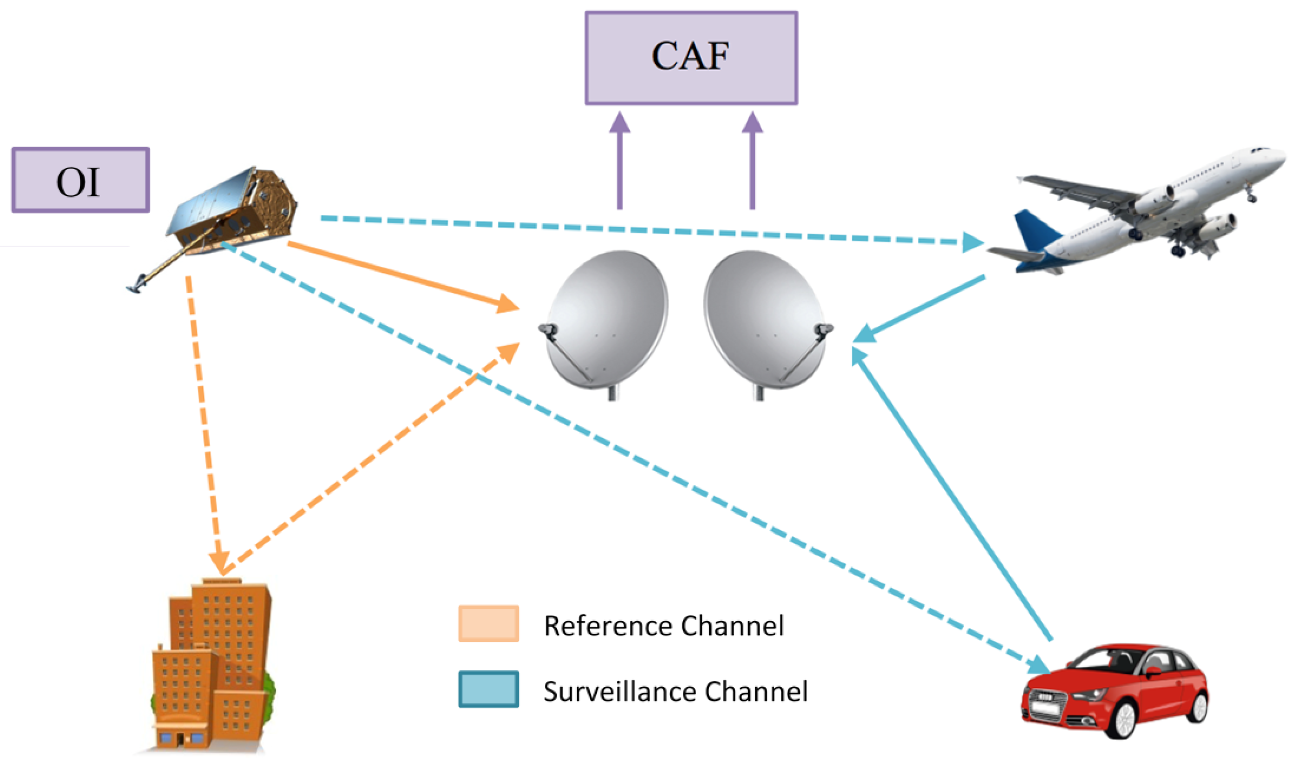
Figure 2, the basic geometry of a bistatic PR using an EO SAR sensor as the OI is presented. The system principle of operation is based on the correlation of the reference signal from the OI acquired by the reference channel (continuous orange arrow) and the target echoes acquired by the surveillance channel (continuous blue arrows). As a result of this coherent processing, the cross-ambiguity function (CAF) is generated.
Figure 2.
Example of passive radar geometry.
Figure 2.
Example of passive radar geometry.
In Equation (
1) the discrete time expression of the CAF is presented for a coherent integration time,
(s), and a sampling frequency,
(Hz), where:
is the number of samples.
m represents the time bin associated with a delay .
p is the Doppler bin corresponding to Doppler shift .
and are the reference and surveillance signals, respectively.
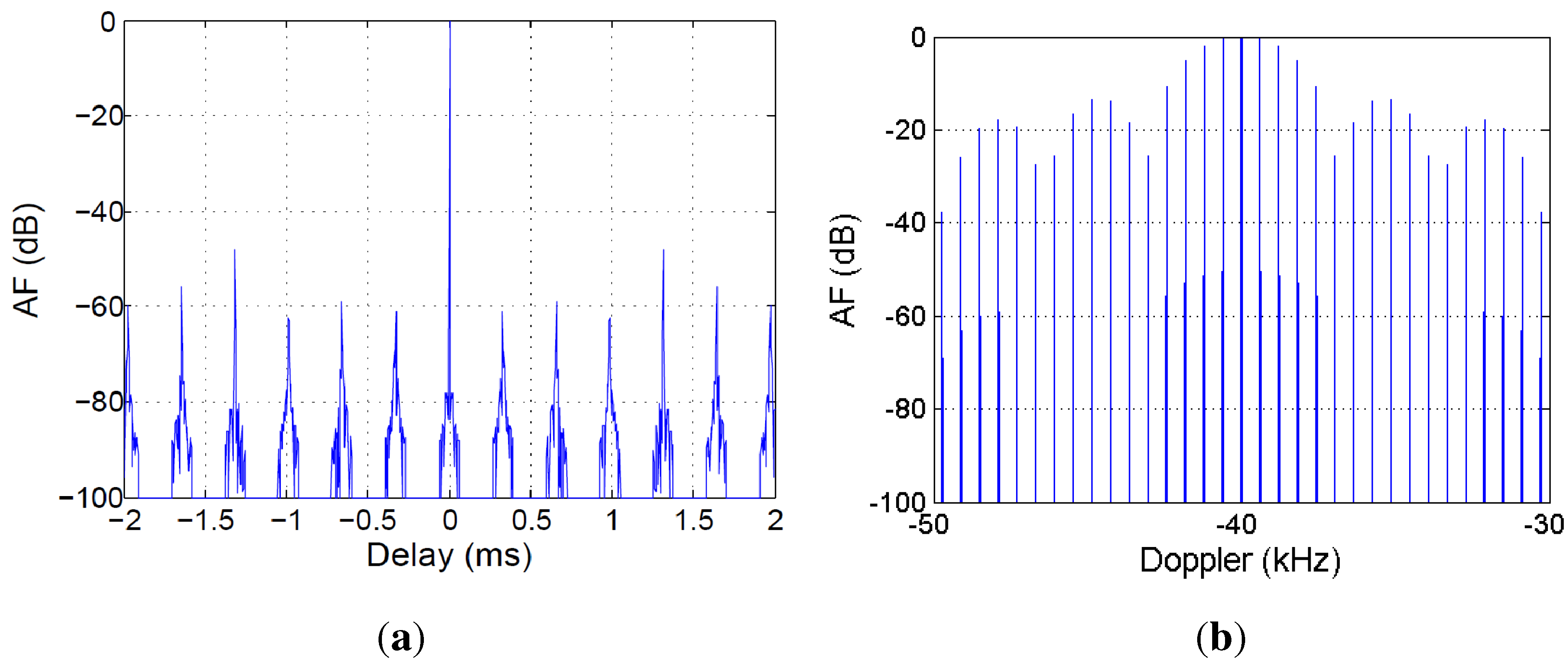
For each target of the coverage area, the result of the CAF is the ambiguity function (AF) of the transmitted signal, scaled and shifted to be centered on the time delay and Doppler shift corresponding to the bistatic range and bistatic Doppler shift of the target.
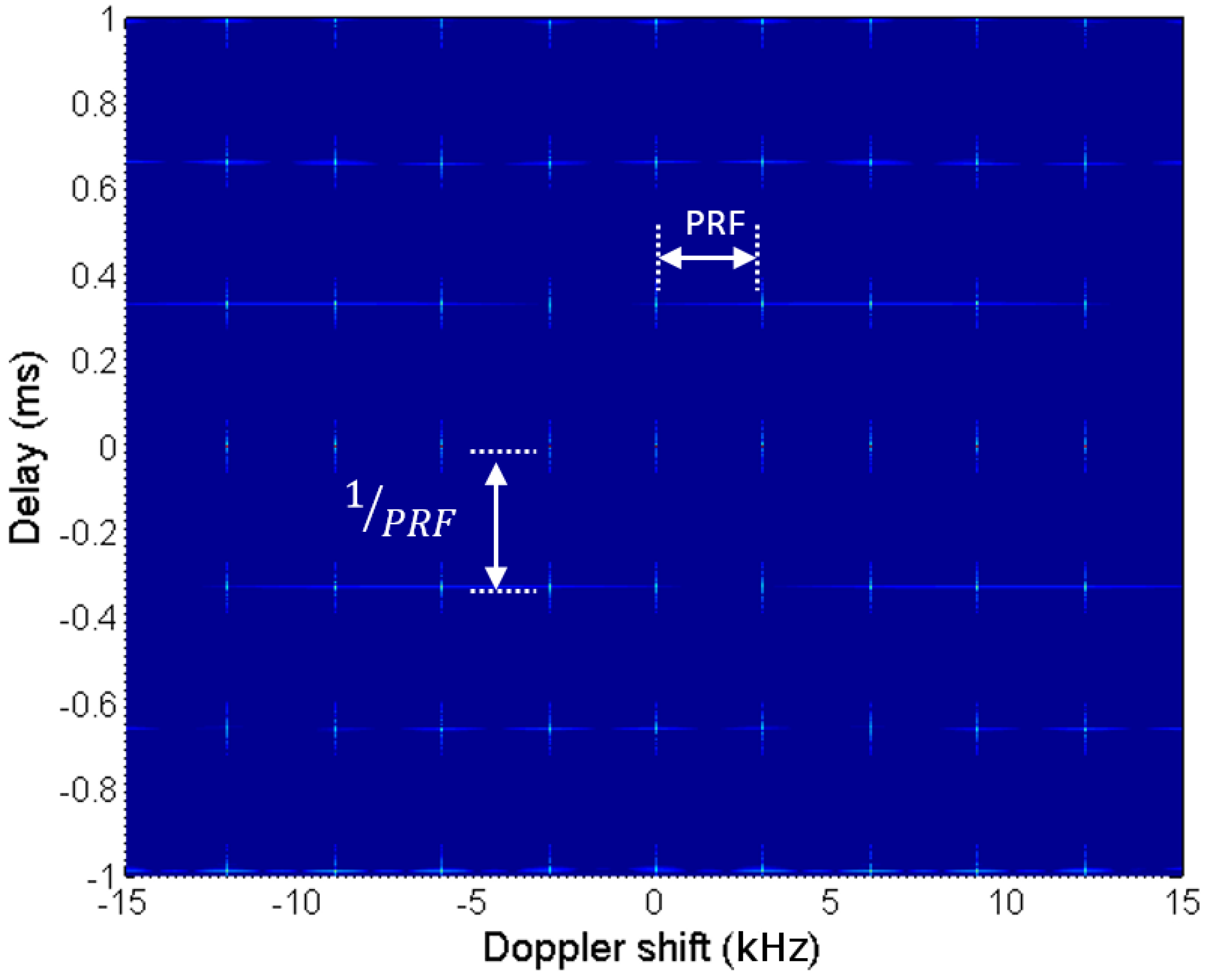
Figure 3 presents an example of CAF generated in a scenario with the following elements:
Two stationary targets are at bistatic ranges
and
. These bistatic ranges are calculated as
, where
is the bistatic delay calculated in Equation (
2) as a function of the target-OI, the target-PR and the OI-PR or baseline distances, denoted as
and
L, respectively.
c is the velocity of light. Stationary targets appear in the zero Doppler line of the range-Doppler map.
One moving target is detected at a bistatic range . Its echo appears in the range-Doppler map at , where is the bistatic Doppler generated by target movement relative to the OI and the PR.
The direct signal transmitted by the OI is captured by the reference and surveillance channels. The surveillance antenna is designed for rejecting this direct signal, but as it can be 100–80 dB higher than the target radar echoes, the level captured by the surveillance antenna can be significant compared to the target echo ones. This signal, known as the direct path interference (DPI) signal, correlates perfectly with the reference antenna signal, and as a result, a peak appears in the range-Doppler map of the CAF, located at zero bistatic range and zero Doppler.
Figure 3.
Example of the cross-ambiguity function (CAF) generated in a scenario with three targets. The effect of the DPI signal is also shown: 3D (a) and 2D (b).
Figure 3.
Example of the cross-ambiguity function (CAF) generated in a scenario with three targets. The effect of the DPI signal is also shown: 3D (a) and 2D (b).
In the following subsections, the main parameters and tools that will be used in the feasibility study are presented: the bistatic range resolution, the bistatic Doppler resolution and the bistatic radar equation.
2.1. Bistatic Range Resolution
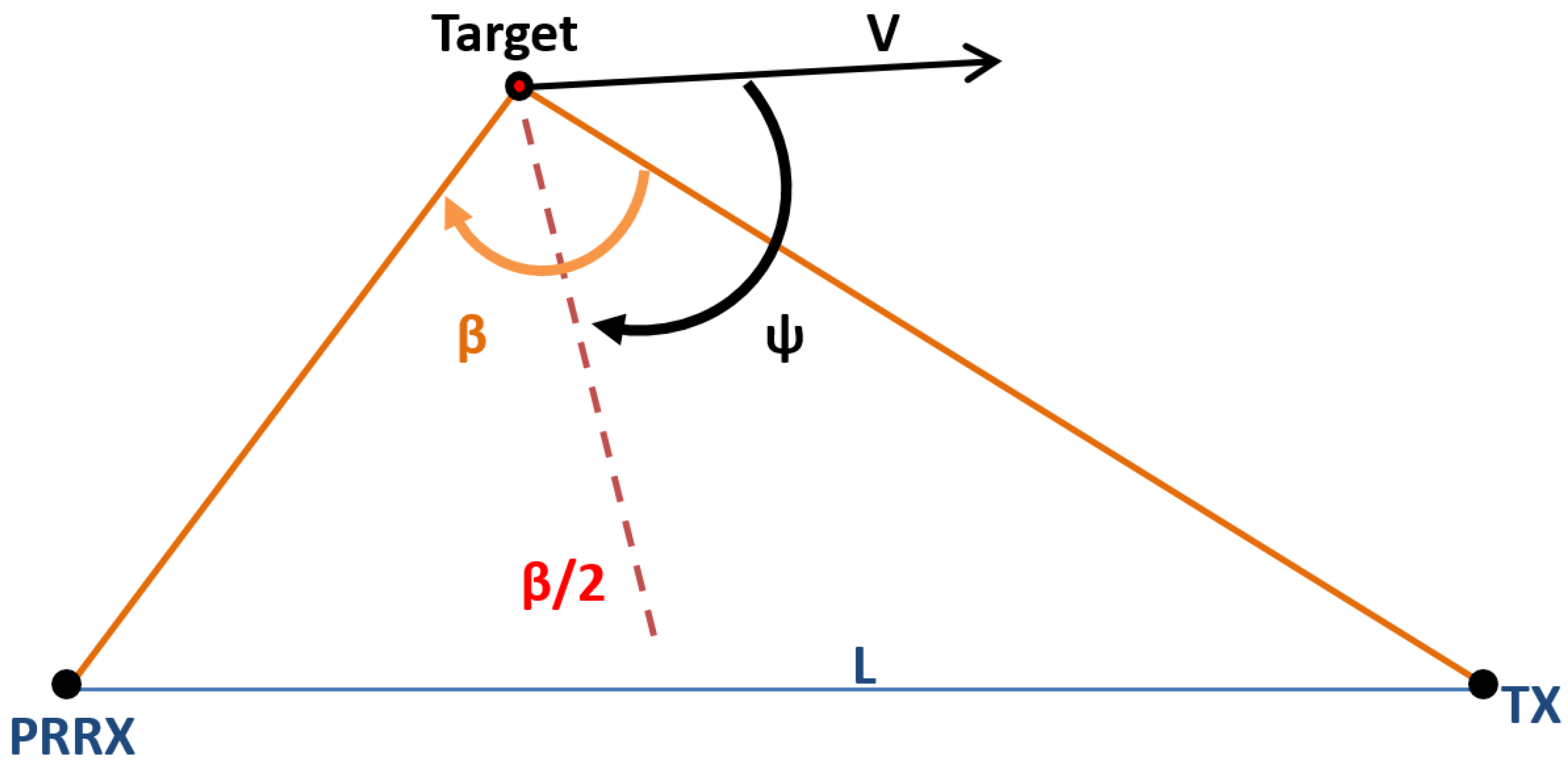
The bistatic range resolution,
, is defined as the minimum distance between two targets that guarantees a time delay between their respective radar echoes equal to the radar compressed pulse width,
. It is calculated using Equation (
3), where
B is the signal bandwidth,
,
β is the bistatic angle,
ψ is the aspect angle with respect to the bistatic bisector and
L is the OI-to-PR or baseline length (
Figure 4). The value obtained for
is usually used for specifying the bistatic range resolution of a system as a function of the bistatic angle.
Figure 4.
Geometry for bistatic range resolution calculation.
Figure 4.
Geometry for bistatic range resolution calculation.
2.2. Bistatic Doppler Resolution
For monostatic and bistatic Doppler resolutions,
is conventionally considered as an adequate Doppler separation between two target echoes at the receiver, where
is the coherent integration time. In
Figure 5, two targets sharing the same bistatic bisector are represented, as well as their speed component along the bistatic bisector. The required
is given by expression Equation (
4) [
1]:
Figure 5.
Geometry for Doppler resolution calculus.
Figure 5.
Geometry for Doppler resolution calculus.
2.3. Bistatic Radar Equation
The radar equation is a mathematical expression that relates the radar range at which the specific performance is obtained to the parameters that characterize the radar (transmitted power, antenna gains, operation frequency, etc.), the desired target (radar cross-section (RCS)) and the radar scenario (bistatic geometry, propagation losses, multipath, clutter).
For the bistatic geometry depicted in
Figure 2, the power scattered by a target can be calculated as:
where
is the received power,
is the power transmitted by the opportunity emitter,
and
are the transmitter and receiver antenna gains, respectively,
λ is the signal wavelength,
A represents the total propagation losses and
and
are the target-to-transmitter and target-to-receiver distances, respectively. The bistatic RCS,
, models the power scattered by the target towards the PR when it is illuminated by the OI.
2.4. System Coverage Limited by Sensitivity
Expression Equation (
5) can be re-written as in Equation (
6). The loci corresponding to
is known as the oval of Cassini. For a required system sensitivity,
, a value of
is obtained.
In the considered bistatic geometry, the passive radar is located on the Earth’s surface (
Figure 6). Assuming a baseline length
km and
km,
, and the Cassini oval breaks into two parts, one centered on the OI and the other on the PR.
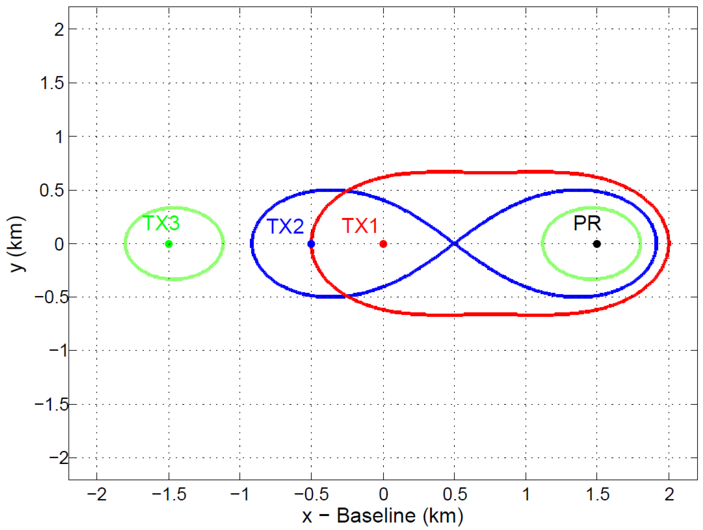
As an example of the impact of the
relation on the coverage area geometry, a simple study is presented in
Figure 7. Assuming a normalized value
km
, different coverage areas are represented for
.
Figure 6.
Geometry of the PAZ-based passive radar: β is the bistatic angle and α is the incidence one.
Figure 6.
Geometry of the PAZ-based passive radar: β is the bistatic angle and α is the incidence one.
Figure 7.
Study of different coverage areas for a fixed passive radar (PR) position as a function assuming km: in red, in blue and in green.
Figure 7.
Study of different coverage areas for a fixed passive radar (PR) position as a function assuming km: in red, in blue and in green.
2.5. Bistatic Radar Cross-Section
The bistatic RCS,
, is a function of the transmitted signal (frequency and polarization), the shape and materials of the target and the incidence and scattering directions. In the bistatic RCS region, characterized by bistatic angles higher than
and lower than
, the bistatic RCS is usually lower than the monostatic RCS for complex targets. Exceptions include [
27]:
Some target aspect angles that generate a low monostatic RCS and a high bistatic specular RCS at specific bistatic angles.
Targets that are designed for low monostatic RCS over a range of aspect angles.
Shadowing that sometimes occurs in a monostatic geometry and not in a bistatic one.
Taking into consideration the scenario geometry depicted in
Figure 6 and the possible incidence and scattering directions, the monostatic and the bistatic RCSs of a car were estimated using the program POFACETS, developed at the Naval Postgraduate School [
28]. Incidence and scattering directions are defined by pairs
, where
θ represents the elevation angle (measured with respect to the Earth’s surface perpendicularly) and
ϕ the azimuth one (measured in the plane tangent to the Earth’s surface, with respect to the north). A basic car model made of perfect electrical conductor (PEC) with dimensions 6 m (L) × 2 m (W) × 1.6 m (H) was used, and the simulations were performed for
GHz and vertical polarization. The RCS has dimensions of area, so an RCS value equal to
corresponds to
.
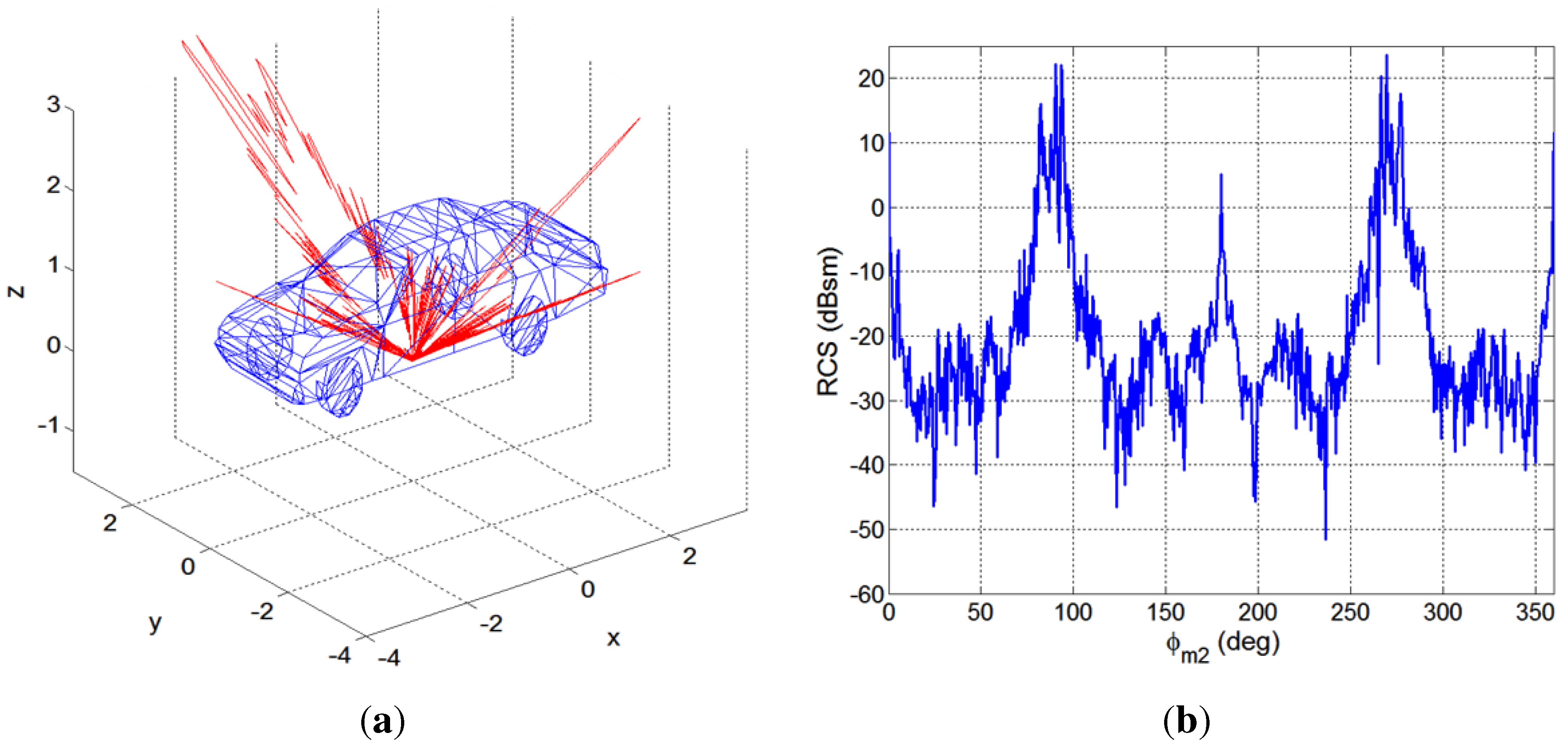
For the monostatic study, two cases were simulated:
Monostatic-1 (
and
), and
Monostatic-2 (
and
). In
Figure 8 and
Figure 9 the results obtained for the monostatic study cases,
Monostatic-1 and
Monostatic-2, are depicted in 3D and in cartesian coordinates.
Figure 8.
Results obtained for the Monostatic 1 case using POFACETS : (a) 3D model of the target and 3D monostatic radar cross-section (RCS); (b) Monostatic RCS in Cartesian coordinates.
Figure 8.
Results obtained for the Monostatic 1 case using POFACETS : (a) 3D model of the target and 3D monostatic radar cross-section (RCS); (b) Monostatic RCS in Cartesian coordinates.
Figure 9.
Results obtained for the Monostatic 2 case using POFACETS: (a) 3D model of the target and 3D monostatic RCS; (b) Monostatic RCS in Cartesian coordinates.
Figure 9.
Results obtained for the Monostatic 2 case using POFACETS: (a) 3D model of the target and 3D monostatic RCS; (b) Monostatic RCS in Cartesian coordinates.
In the bistatic case, incidence and scattering directions must be considered. The estimation of an average bistatic RCS was performed using the following methodology:
For each value of incidence elevation angle, and , the incidence azimuth angle, , was varied from to , taking into consideration the symmetry of the car in the XY plane.
For each incidence direction
, the elevation angle of the scattered wave was fixed to
, and the azimuth scattering angle,
, was varied from
to
.
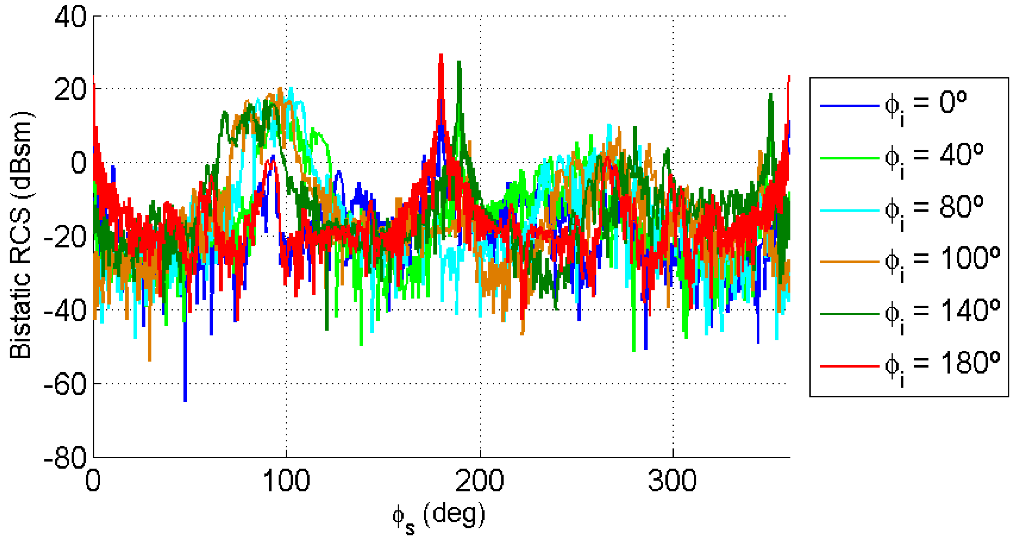
Figure 10 and
Figure 11 show results obtained for
and
, respectively.
Figure 10.
Bistatic RCS as a function of the scattering direction azimuth, , for , and .
Figure 10.
Bistatic RCS as a function of the scattering direction azimuth, , for , and .
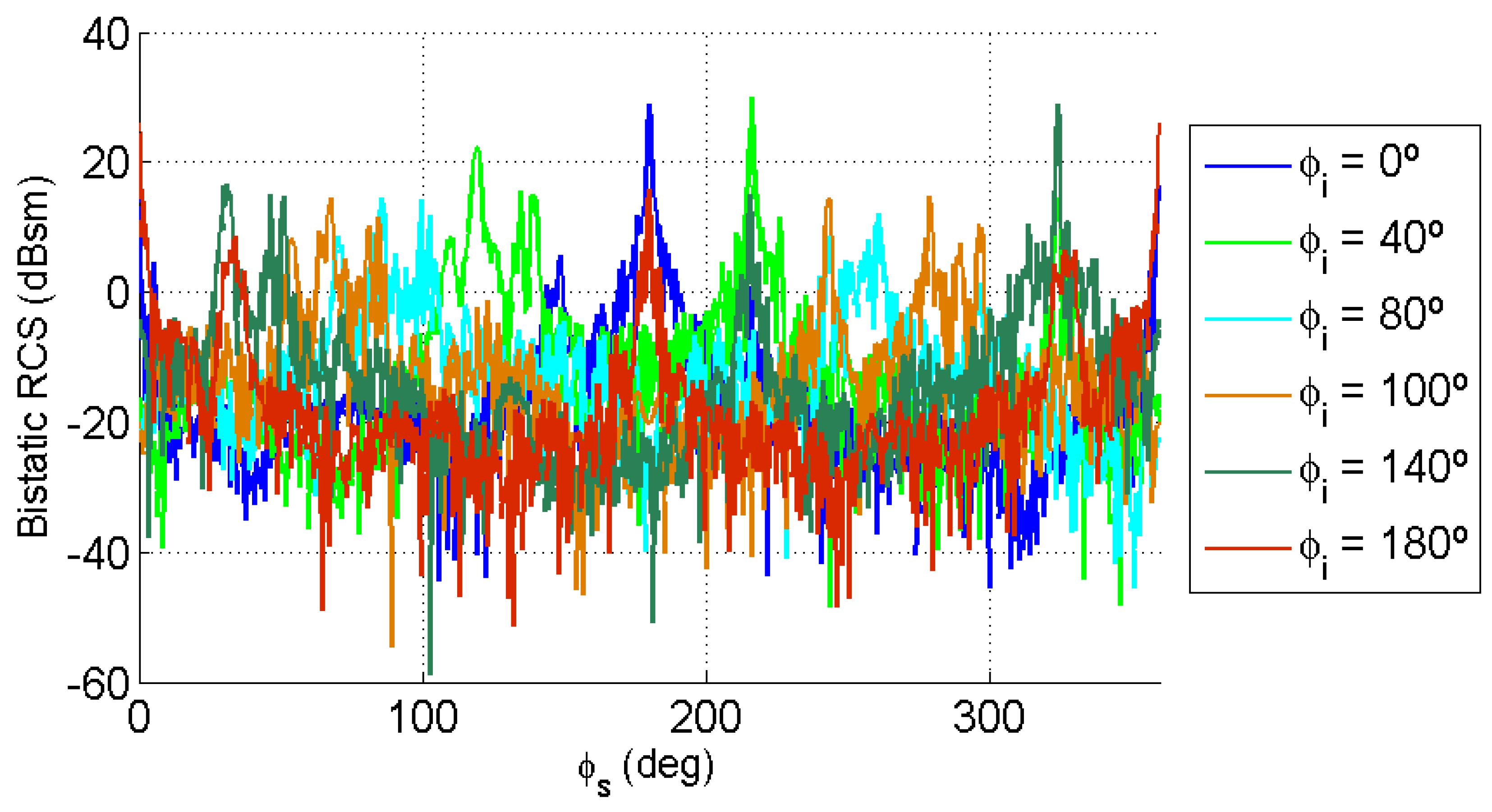
Figure 11.
Bistatic RCS as a function of the scattering direction azimuth, , for , and .
Figure 11.
Bistatic RCS as a function of the scattering direction azimuth, , for , and .
For each scattering direction,
, and incidence elevation angle
, an average bistatic RCS was calculated as the mean value of the bistatic RCSs estimated for the set of
values ranging from
to
. The study carried out for
was denoted as
Bistatic-1 and the study for
was denoted as
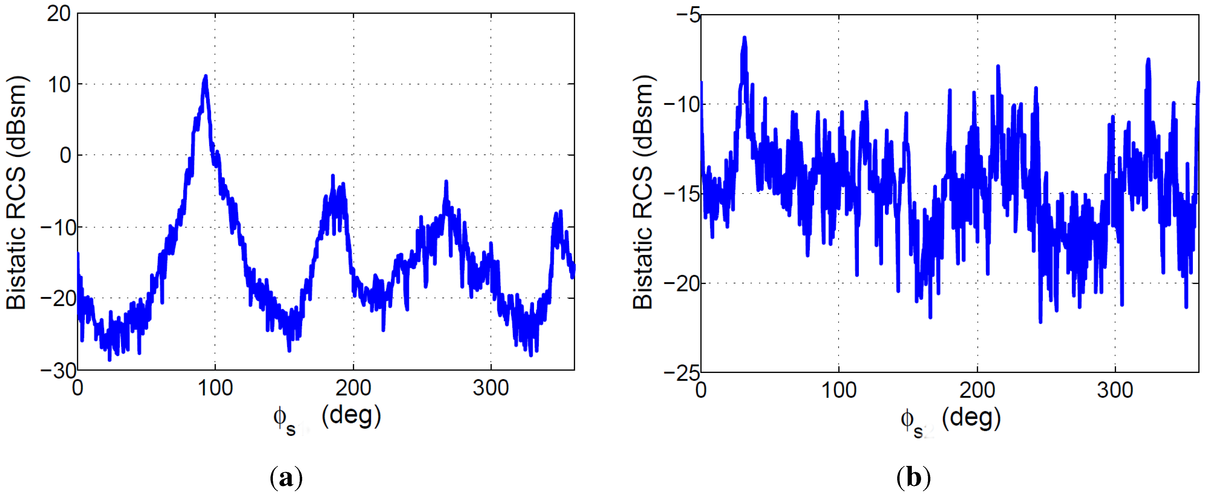
Bistatic-2. Results are presented in
Figure 12.
Maximum, minimum and average values of the mean bistatic RCS along the
dimension are summarized in
Table 1. Results show that for the lower incidence angle (close to normal incidence), the monostatic RCS is higher than the bistatic one, but for higher values of the incidence angle, the bistatic RCS can be higher than the monostatic one.
Figure 12.
Bistatic RCS averaged along the incidence direction azimuth, : (a) Bistatic 1 case study; (b) Bistatic 2 case study.
Figure 12.
Bistatic RCS averaged along the incidence direction azimuth, : (a) Bistatic 1 case study; (b) Bistatic 2 case study.
Table 1.
Bistatic RCS simulations results.
Table 1.
Bistatic RCS simulations results.
| RCS | Monostatic 1 | Bistatic 1 | Monostatic 2 | Bistatic 2 |
|---|
| Maximum | 37.385 dBsm | 11.074 dBsm | 23.611 dBsm | −6.293 dBsm |
| Minimum | −50.229 dBsm | −28.678 dBsm | −51.619 dBsm | −22.193 dBsm |
| Average | −3.331 dBsm | −15.522 dBsm | −20.532 dBsm | −14.658 dBsm |
3. PAZ Description
The PAZ satellite platform is similar to the TerraSAR-X one and has been developed by Airbus DS. The instrument front-end has been designed by Airbus DS Spain/CASAEspacio ( Construcciones Aerospaciales S.A.). The Spanish National Institute for Aerospace Technology (INTA, Instituto Nacional de Tecnología Aerospacial) has been responsible for the development of the Ground Segment of the PAZ Mission, and it is responsible for PAZ scientific exploitation.
Scientific exploitation conveys all knowledge areas related to SAR technology: radio-frequency, digital signal processing, image processing, remote sensing,
etc. The main objectives are the following:
To identify areas of interest considering the Spanish environment and compromises.
To provide data to the scientific community for educational, scientific and technological purposes.
To research SAR systems’ characterization and calibration, operating modes’ definition, multi-static configurations and multi-sensor developments.
To collaborate with high level SAR institutions.
To develop a set of research-based demonstrators to prove SAR technology capabilities in different applications.
Searchers or research groups can communicate their interest to the e-mail address
[email protected].
For the proposed study, the antenna gain and the imaging modes are of great importance. They are analyzed in the following subsections.
3.1. PAZ Antenna
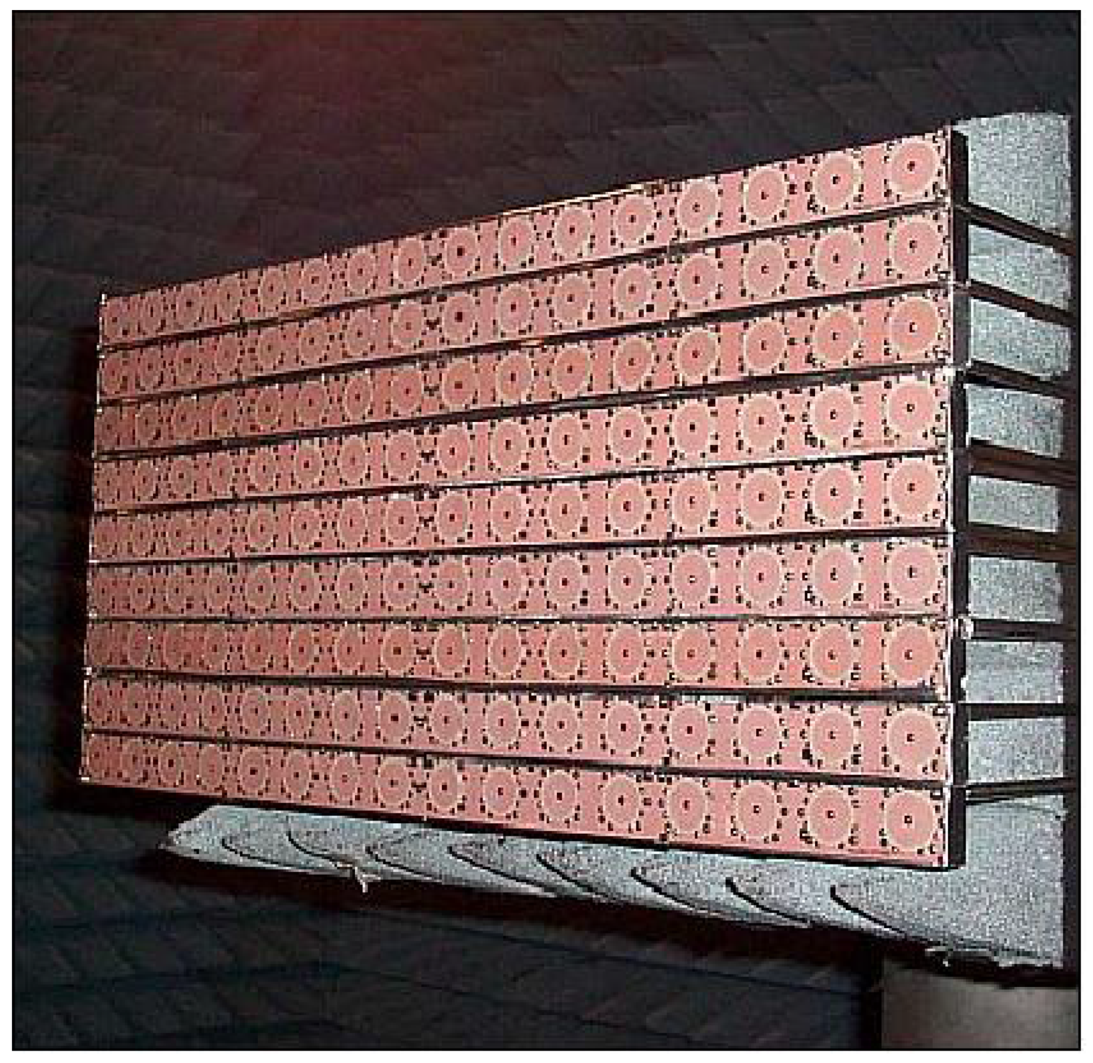
The PAZ antenna is an X-band active-phase planar array implemented in printed-radiator technology. Together with a low profile, low-mass, flexibility and easiness of manufacturing, this technology allows the development of flexible beamforming networks (BFN).
The PAZ planar array is composed of 12 panels (4.8 m × 0.7 m). Each panel is composed of 32 subarrays, and each subarray is composed of 16 microstrip patches. Each subarray is a single radiating element, which includes a dedicated transmit-receive module (TRM) adjustable in amplitude and phase by applying complex excitation coefficients. This enables beam steering, adaptive beamforming in the azimuth and elevation and the generation of more than ten thousand beams. An accurate antenna model (AMOR, Antenna MOdelleR ) was developed for generating the antenna patterns for improving radar image quality and calculating TRM settings to ensure the performance further on, even in the case of drifting and/or failed modules during the spacecraft lifetime, among other objectives [
29].
Figure 13 shows a qualification model composed of nine subarrays [
8].
Figure 13.
PAZ panel subarrays [
8].
Figure 13.
PAZ panel subarrays [
8].
The array gain is a key element in the feasibility study, so an estimated value was calculated using the available information [
30]:
Assuming that all of the elements of the array are equal and unaffected by the position in the array, thus ignoring some possible edge effects, the array gain can be estimated as follows [
31]:
where:
is the element efficiency term due to possible mismatching effects.
represents the scan loss effect, which is typically modeled as a function of , being the main beam pointing direction with respect to the array broadside direction.
represents the directivity of each single radiating element.
N is the number of single radiating elements in the array.
Given the similarities between PAZ and TerraSAR-X, the angle between the array panel inclination and nadir direction of TerraSAR-X was considered for the study, this value being equal to .
Finally, the Equivalent Isotropic Radiated Power (EIRP) was estimated for α ranging from to . For and . EIRPs of dBm and dBm, were obtained, respectively.
3.2. Transmitted Signal
The PAZ signal is a periodic train of linear frequency-modulated pulses. The typical bandwidth will be 150 MHz, but it will be able to be increased to 300 MHz for special imaging modes.
Table 2 summarizes the main signal parameters [
32,
33].
Table 2.
PAZ signal parameters.
Table 2.
PAZ signal parameters.
| Central frequency | 9.65 GHz |
| Maximum bandwidth | 300 MHz |
| Peak power | 1.9 kW |
| Pulse length | 15 µs–67 µs |
| Service factor | – |
| Pulse repetition frequency | 2 kH– kH |
3.3. Orbit Parameters
PAZ will fly in a polar dawn-dusk Sun-synchronous orbit. This type of orbit allows power throughput maximization and simplifies the thermal design. TerraSAR-X and TanDEM-X satellites follow this same orbit, offering the capability for repeat-pass interferometry. PAZ will cover all of Earth with a mean revisit time of one day and a mean access delay slightly higher than 24 h (
Table 3) [
33].
Table 3.
PAZ orbit and incidence angle values.
Table 3.
PAZ orbit and incidence angle values.
| Nominal height | 514 km |
| Orbits per day | 15 + 2/11 |
| Incidence angle | 20–45 (full perf.) 15–60 (accessible) |
3.4. PAZ Imaging Modes
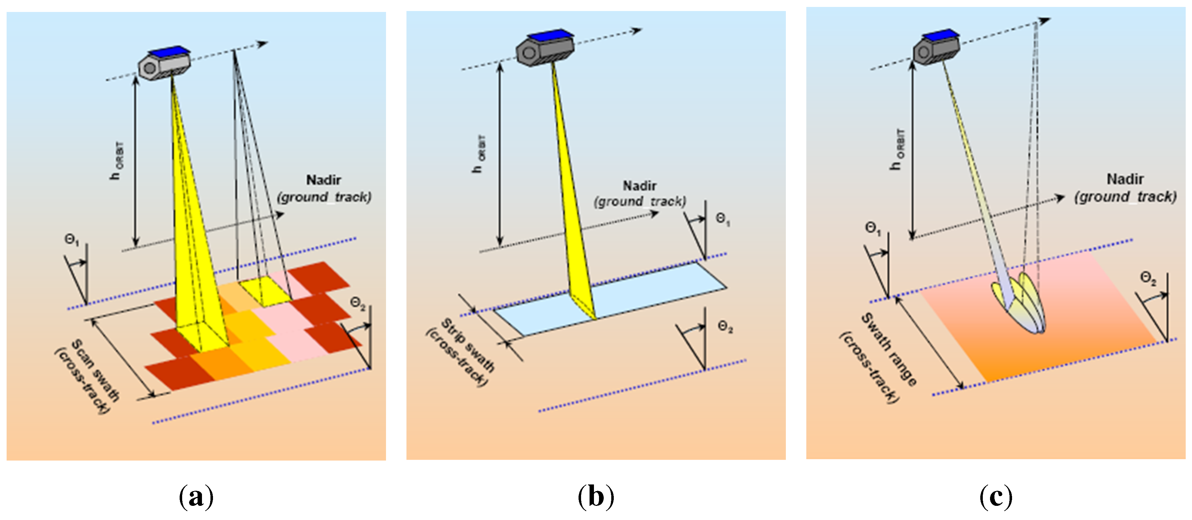
The PAZ satellite will operate in four nominal imaging modes (
Figure 14):
Stripmap: The antenna beam is pointed to a fixed angle in elevation and azimuth, resulting in a strip with constant quality in azimuth (azimuth resolution up to 3 m, scene size up to 30 km × 50 km). Single (HH, VV) and dual (HH/VV, HH/HV, VV/VH) polarization modes are possible.
ScanSAR: The electronic antenna elevation steering is used to switch after bursts of pulses between swathes with different incidence angles. This mode has an azimuth resolution up to 18 m, with a scene size of 100 km × 150 km. It can only acquire images with single polarization (HH, VV).
Spotlight: Azimuth phased array beam steering is used to increase the illumination time and the azimuth resolution, at the cost of azimuth scene size (azimuth resolution up to 2 m, scene size of 10 km × 10 km). Single (HH, VV) and dual polarization (HH/VV) operating modes are possible.
High resolution spotlight: this mode has an azimuth resolution up to 1 m, with a scene size of 10 km × 5 km and is able to operate with single (HH, VV) and dual polarization (HH/VV).
New modes developed for TerraSAR-X, such as the staring spotlight and the wide ScanSAR, are foreseeable for PAZ.
Figure 14.
PAZ imaging models [
8]: ScanSAR (
a); stripmap (
b); spotlight (
c).
Figure 14.
PAZ imaging models [
8]: ScanSAR (
a); stripmap (
b); spotlight (
c).
5. Case Study Example
The analysis of the bistatic geometry of a PR based on TerraSAR-X was carried out, because of the similar characteristics of PAZ and TerraSAR-X. The central point of the area of interest was located at the University of Alcalá campus, on the roof of the Polytechnic School, with the following coordinates N, W and an altitude of 587 m.
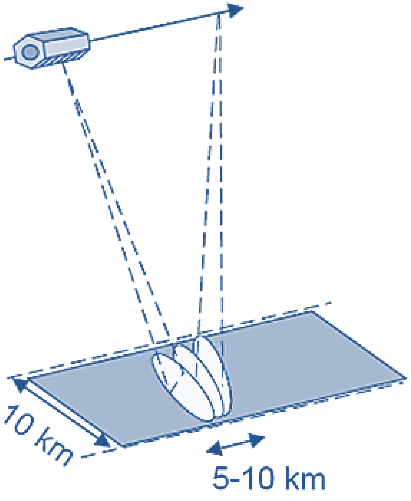
An acquisition in spotlight mode was assumed. This mode simplifies the geometry of the system, because it allows the definition of a constant coverage area during SAR sensor operation. It has been selected in order to focus on the description of the parameters to be considered in the analysis. Once the methodology has been explained, it can be straightforwardly applied to ScanSAR and stripmap modes, taking into consideration the movement of the footprint and the increase in the achievable coverage area.
A spotlight image acquisition covering an area of
km
, with a bandwidth of 300 MHz, an incidence angle of
, and an acquisition time of
s was assumed (
Figure 18). Due to the slight movement of the beam along the cross-range direction, an effective inner illuminated area of
km
was considered (
Figure 20).
The PR receiver was located at the center of the area of interest. This solution minimized the required sensitivity, taking into consideration that, as has been already mentioned, the coverage was composed of two independent ovals centered on the OI and the PR receiver, respectively. The considered area laid completely in the unambiguous detection region defined by the LFM pulse train CAF, which is around 480 km long for the monostatic case.
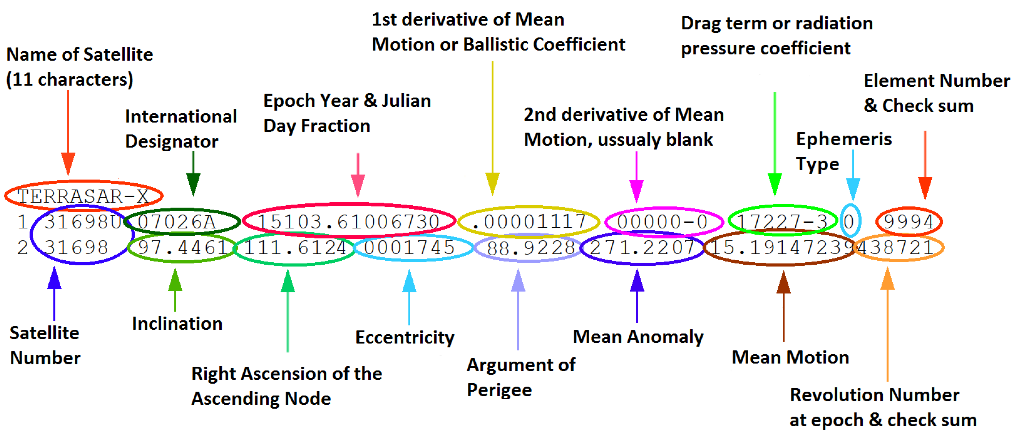
The date and time parameters of the case of study were: 13 April 2015, 17:58:50. From the TLE parameters provided by the SGP4 model, during the acquisition time of
s, the main features of the satellite movement where estimated:
The satellite moved from N, W to N, W.
Satellite altitude remained approximately constant and equal to 513.4 km.
The acquisition started at the time when the elevation angle of the satellite with respect to the PR receiver location was maximum. The elevation variations were of some hundredths of degree around .
The azimuth of the satellite with respect to the North varied , from to . This variation was higher due to the polar orbit of the sensor.
Knowing the position of the OI during the acquisition time, a bistatic system geometry analysis was carried out throughout the coverage area (
Figure 20) with the following considerations:
The area of interest was divided into m cells.
The system geometry was calculated assuming that a non-moving ground target was located at the center of each cell.
The system geometry was recalculated each 0.01 s (150 time slots were analyzed) in order to take into account the satellite dynamics.
Figure 20.
Case study geometry analysis scheme.
Figure 20.
Case study geometry analysis scheme.
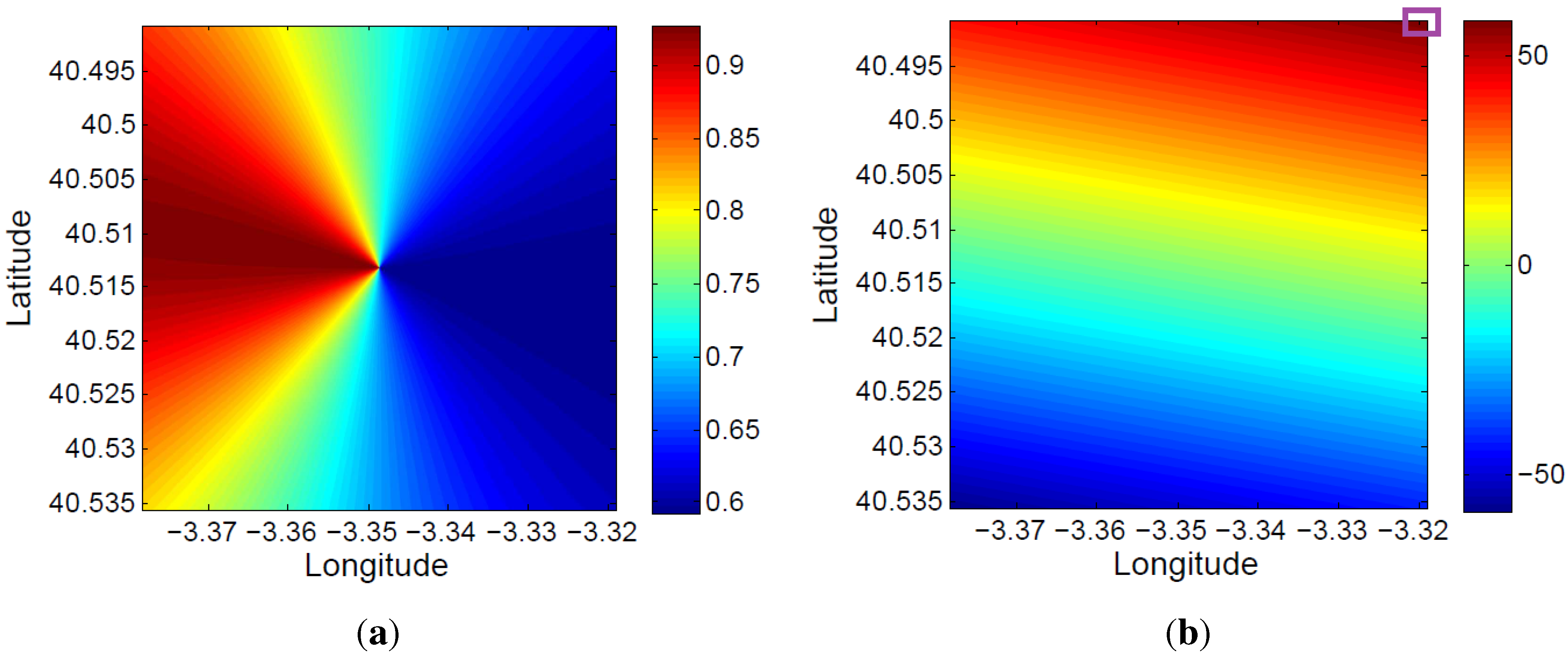
The bistatic angle at the acquisition starting time for each
m
cell of the defined coverage area is presented in
Figure 21a. The total variation of the bistatic angle during the whole acquisition time is represented in
Figure 21b. The maximum bistatic angle variations is equal to
.
Figure 21.
Study of the spatial and time variation of the bistatic angle: (a) initial value at each m cell of the coverage area; (b) total variation during the acquisition time.
Figure 21.
Study of the spatial and time variation of the bistatic angle: (a) initial value at each m cell of the coverage area; (b) total variation during the acquisition time.
The bistatic range resolution, which is a function of the bistatic angle, was also analyzed. Using Equation (
3), its value at the acquisition starting time for each
m
cell of the defined coverage area was calculated (
Figure 22a). Due to the small variation of the bistatic angle during the acquisition time, the variation of the bistatic range resolution in the
s has not been represented.
Because of the satellite movement, the bistatic time delay and the associated bistatic range are also a function of time (
, in
Figure 6). This makes the estimated target location a time-dependent variable. In
Figure 22b, the total variation of the bistatic range during the whole acquisition time is represented for each
m
cell of the defined area of coverage. In this case, variations of 50 m are calculated.
Figure 22.
Bistatic range resolution and bistatic range: (a) initial bistatic range resolution at each m cell of the coverage area; (b) total variation of the bistatic range during the acquisition time.
Figure 22.
Bistatic range resolution and bistatic range: (a) initial bistatic range resolution at each m cell of the coverage area; (b) total variation of the bistatic range during the acquisition time.
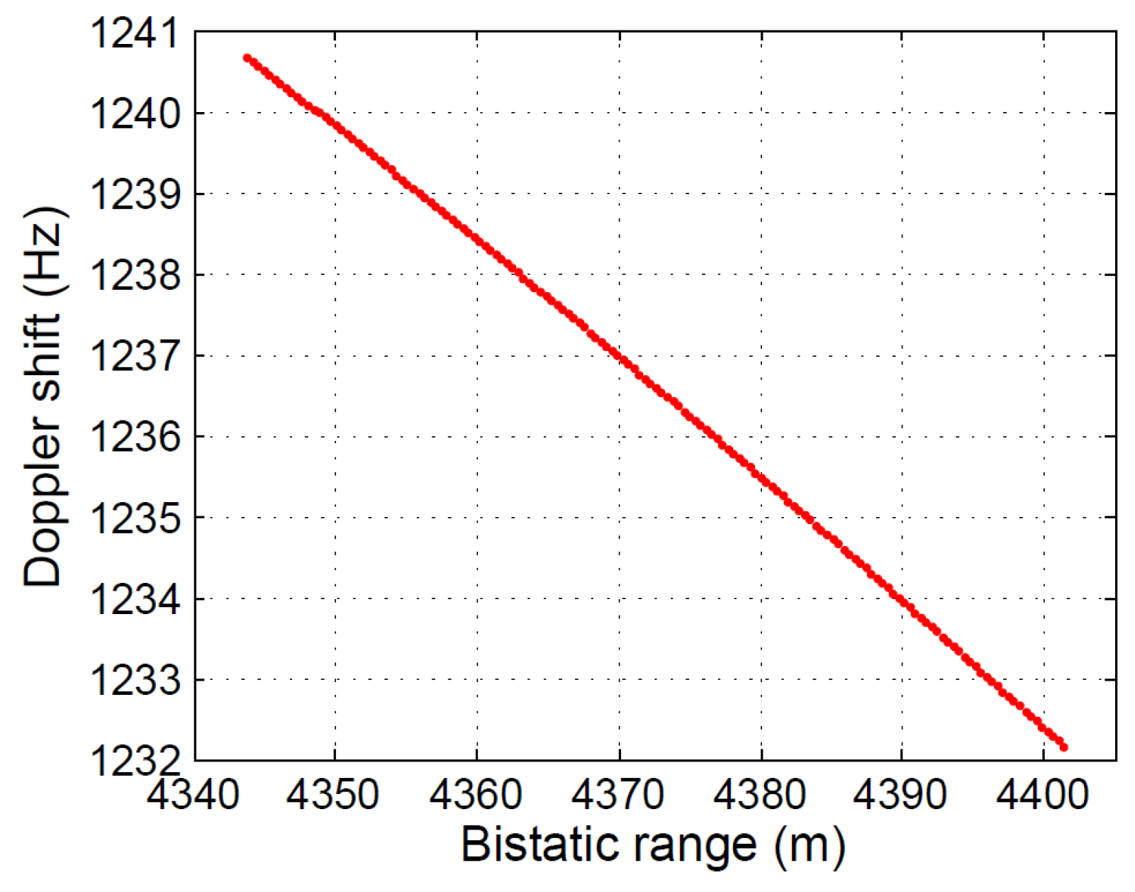
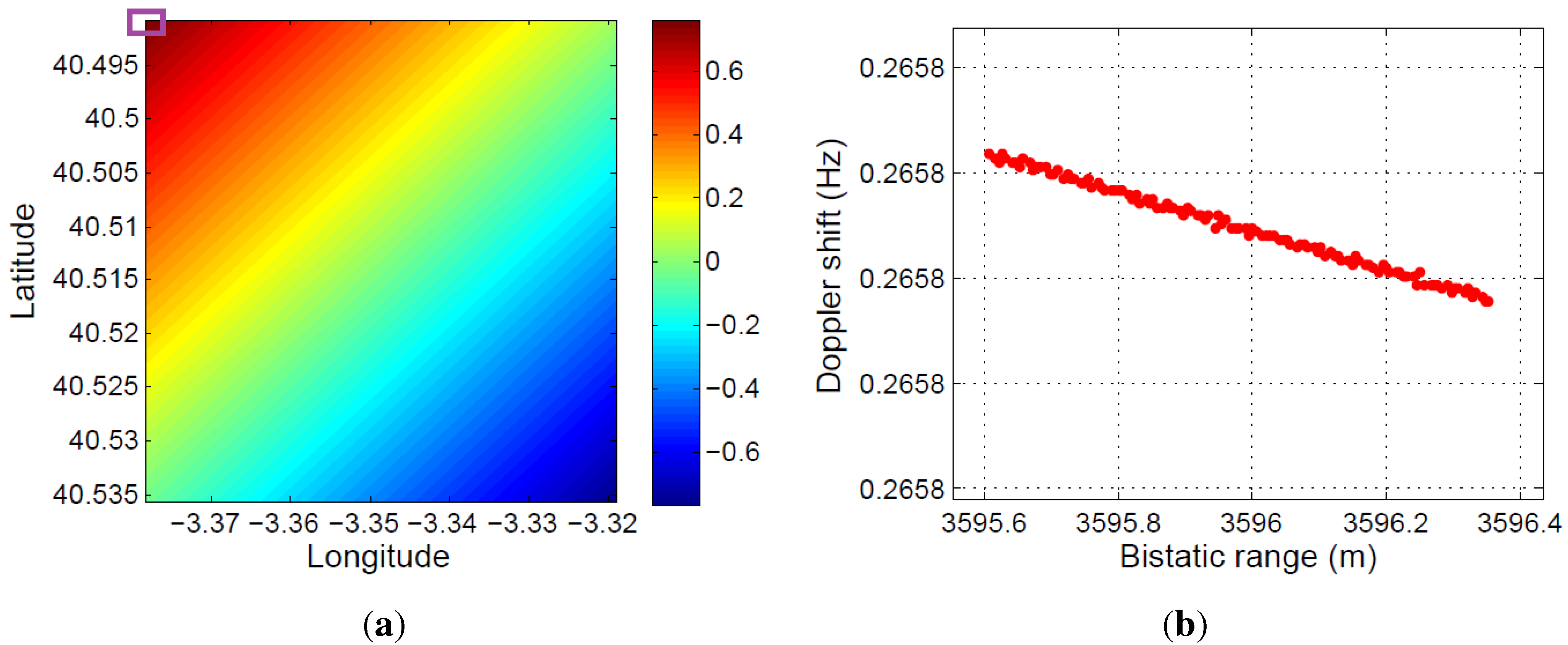
The variation of the bistatic range with time for a stationary target (
i.e., corner reflector) located at the center of a
m
cell gives rise to the virtual movement of the stationary target. In
Figure 23, the virtual trajectory of a stationary target located at the upper right corner cell of
Figure 22b is depicted. During the acquisition time, an average speed of 38 m/s and a total variation of the bistatic range of around 55 m were estimated.
Figure 23.
Virtual displacement for a fixed point inside the area of interest.
Figure 23.
Virtual displacement for a fixed point inside the area of interest.
This virtual movement is completely defined by the system geometry, so it can be predicted and, therefore, compensated. To complete the study, two examples of different system geometries are presented:
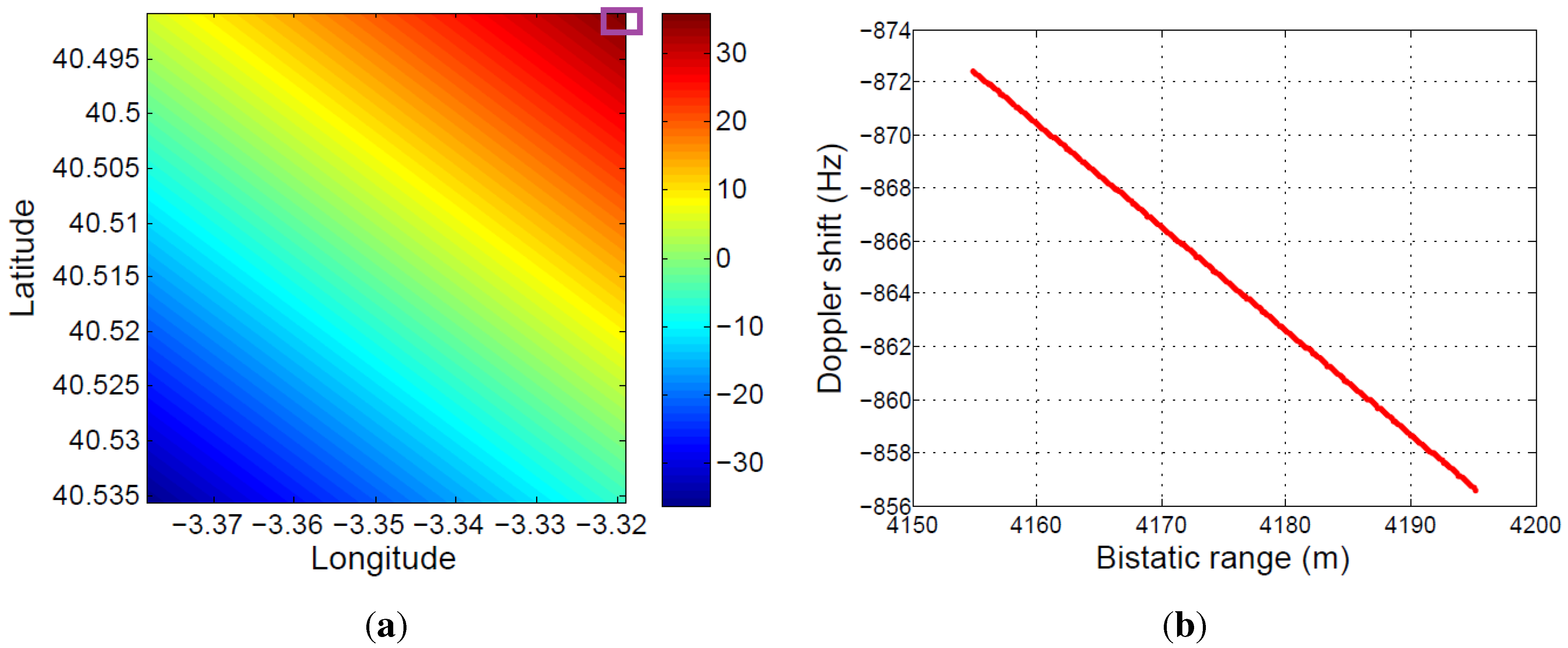
Virtual movement analysis for a bistatic radar scenario using the same satellite, but assuming a different acquisition date: The new date and time parameters are: 3 June 2015, 17:34:15.
Figure 24 shows the total variation of the bistatic range and the virtual movement of the same stationary target as in the previous study, during the same acquisition time. In this case, the maximum magnitude of the bistatic range variation is approximately 35 m, lower than the approximated 55 m obtained in the previous study.
Figure 24.
System geometry analysis assuming different TerraSAR-X orbital parameters (3 June 2015, 17:34:15): (a) total variation of the bistatic range during the acquisition time; (b) virtual displacement associated with satellite movement.
Figure 24.
System geometry analysis assuming different TerraSAR-X orbital parameters (3 June 2015, 17:34:15): (a) total variation of the bistatic range during the acquisition time; (b) virtual displacement associated with satellite movement.
Virtual movement analysis for a bistatic radar scenario using a GPS satellite: A new study case is considered exploiting the signal transmitted by Navstart 59 (USA 192). This is a medium-orbit satellite. The date and time parameters are: 25 May 2015, 12:20:00. The characteristics of the orbit and the transmitted signal parameters used in the study are summarized in
Table 5 and
Table 6, respectively. Results are presented in
Figure 25. In this case, the stationary target is assumed to be located on the upper left corner of
Figure 25a, in order to perform the analysis for a case characterized by a big variation of the considered parameters. For the same acquisition time used in previous examples, the obtained virtual displacement is significantly lower, less than 1 m.
These results validate the proposal of a PAZ-based PR for PAZ calibration and maintenance purposes and for surveillance of critical areas where the increase of monitoring time and/or target speed estimation could be important added values.
Table 5.
GPS signal parameters used in the third geometry study.
Table 5.
GPS signal parameters used in the third geometry study.
| Central frequency | 1557 MHz |
| Bandwidth | 2 MHz |
| Power | 27 W |
| Modulation | Spread spectrum |
| Transmission rate | 50 bps |
Table 6.
GPS orbit parameters.
Table 6.
GPS orbit parameters.
| Nominal height | 20,200 km |
| Orbits per day | 2 |
Figure 25.
System geometry analysis for Navstart 59 (USA 192), on 25 May 2015, at 12:20:00: (a) total variation of the bistatic range during the acquisition time; (b) virtual displacement associated with the satellite orbit.
Figure 25.
System geometry analysis for Navstart 59 (USA 192), on 25 May 2015, at 12:20:00: (a) total variation of the bistatic range during the acquisition time; (b) virtual displacement associated with the satellite orbit.
6. Conclusions
PAZ, the satellite EO SAR sensor of the Spanish National Earth Observation Program, is a powerful observation tool that will be used in the different applications defined in Copernicus, the European Earth observation program: land monitoring, marine monitoring, emergency management and security.
Taking into consideration the increasing interest in passive radars and the potential good features of a system such as PAZ, a complete study about PAZ’s feasibility as an opportunity illuminator in passive radar applications was carried out. Bistatic SAR systems have been the object of study, and some works dealing with the generation of passive radar images have been published. In this paper, the feasibility of PAZ as an opportunity illuminator in a passive bistatic radar system in surveillance applications was considered. Although a major drawback of that system is its intermittency in acquisition, constrained by the orbit parameters and its on-demand operating principle, PAZ is a powerful detection tool, with a finite lifetime, factors that justify the search for alternative applications.
A detailed study was carried out to analyze the influence of waveform, platform movement, variable bistatic geometry, transmitted power and on-demand operation mode. The main conclusions are the following:
The transmitted signal is characterized by periodic ambiguity peaks that limit the coverage area and the target dynamics. After a study of instrumented coverage and system sensitivity, the limits imposed by the signal AF are beyond the limits imposed by these other factors, so the ambiguity peaks have no practical effect on system performance.
OI availability: A study of potential bistatic geometries was carried out in order to determine the time availability and the instrumented spatial coverage. The orbital parameters, the acquisition modes and the operation schedule impose critical limitations on the OI availability. Taking into consideration these limitations, the following potential applications are proposed:
- −
A PR system exploiting the signal emitted by PAZ can be used as a low-cost, easily deployable and configurable calibration tool in the commissioning phase of the SAR sensor or in posterior maintenance processes. The cost associated with the PR receiver is expected to be reduced due to the availability of commercial systems for direct receiving of sensor X-band data.
- −
PR based on PAZ can also provide additional information, especially that related to the speed and trajectory of moving targets, to improve the information extraction from the acquired SAR images in the operational phase. This application can be really important in areas of special interest for monitoring specific phenomena.
- −
As a PR can exploit the signal transmitted by other SAR sensors, GNSS and communication satellites, BSAR images can be generated to fill time gaps during which PAZ is not available.
Instrumented coverage area: This is determined by the OI antenna footprint. The spotlight acquisition mode simplifies the geometry of the system, because it allows the definition of a constant coverage area during SAR sensor operation. For stripmap or ScanSAR operation, the knowledge of the sensor position makes it possible to study the movement of the coverage area, providing an increase of the achievable coverage.
Different study cases were defined to analyze the impact of OI orbit: two study cases based on TerraSAR-X with different orbit parameters and a study case based on a GPS satellite.
Incident power density and required sensitivity: The available power at the PR antenna was estimated as a function of the target-to-PR distance, proving the feasibility of PAZ as an IO from this point of view, allowing coverages of 15 km with affordable system sensitivities.


