1. Introduction
Relative navigation of a non-cooperative target satellite is an important part of space missions such as space offense and defense, on-orbit maintenance and orbital debris removal [
1,
2]. Different from the relative navigation of a cooperative target in which special optical markers are equipped on the target [
3,
4], the non-cooperative target has no preset special marker to be used. Since satellites are artificial objects, they usually have obvious feature points such as edges and corners on their surfaces, and these feature points can be used to obtain the relative navigation information [
5]. If all of the feature points extracted from the surface of the target satellite are used for the relative navigation, the computational load will be very large. It is a great challenge for the chaser satellite with limited computing ability or a high real-time requirement. Therefore, a compromise between the computational load and the performance should be explored in practice. From this point of view, a subset of feature points can be selected for the relative navigation. The number of selected feature points should be far less than the number of the total feature points to reduce the computational load. Meanwhile, the accuracy with the selected feature points should meet the navigation requirement.
The estimated variance in a vision-based navigation system is closely related to the geometric distribution of feature points [
6]. The accuracy can be described by the dilution of precision (DOP), which is widely used in the Global Navigation Satellite System (GNSS) [
7,
8,
9]. A smaller DOP value indicates a higher navigation accuracy. For a vision-based navigation system that estimates position and attitude simultaneously, the geometric distribution of feature points affects the accuracies of position and attitude. Therefore, the accuracies of position and attitude can be described by position DOP (PDOP) and attitude DOP (ADOP), respectively.
The DOP of the vision-based system have been studied in recent years. Baine [
10] studied the DOP of the vision-based system using the directional cosine matrix in the navigation frame and applied it to the consistency test. Park [
11] studied the DOP of a combined vision and IMU system taking into account the alignment error and the mapping error, then analyzed the characteristics of the DOP in this system. Won [
12] derived the weighted DOP using the unit vectors of feature points when the variances of feature points were different with respect to the geometrical distortion of the vision sensor. These research works were concerned with the DOP of absolute navigation and took the target body frame as the reference frame. To estimate the position and attitude of the non-cooperative target satellite, the DOP for the relative navigation in the sensor frame should be studied.
With the concept of DOP, the problem of the feature point selection for the non-cooperative target satellite can be described as selecting
m from
n feature points to make the DOP value as small as possible, where
m represents the number of selected feature points and
n represents the number of the total feature points. The most straightforward method called the optimal method [
13] is to calculate the DOP values of all possible combinations with the number of
m, then the subset with the minimum DOP value is selected. In this method, all possible combinations of
m from
n are tested, and each combination has matrix multiplication and inversion. The corresponding number of combinations is
. For example, if
and
, then there will be almost
combinations to be tested. The number of combinations rapidly increases with the increase of the total feature points, and it is unacceptable for the chaser satellite to complete the computation.
The feature point selection in a vision-based navigation system is similar to the satellite selection in GNSS. In GNSS, more and more satellites are in view because of the advent of Galileo, Compass and GPS. The increase of satellites will make use of the optimal method intractable. Many scholars have proposed different satellite selection methods in GNSS including the recursive method [
14], maximum volume method [
15,
16], four-step method [
17], neural network method [
18,
19] and other methods [
20,
21,
22,
23]. Since these methods utilize the characteristics of satellite orbit such as longitude and latitude or have a restriction on the selected number, they cannot be used to select feature points in a vision-based navigation system.
The image cannot be used to select feature points in different planes directly because of the lack of three-dimensional information. This paper assumes that feature points are in a plane. They can be easily obtained at close range navigation or based on the structure model of the target satellite, which is known in advance. Thus, the distribution of the feature points on the surface of the target satellite is similar to the distribution of the feature points on the image. The feature point selection is to select feature points on the image.
Inspired by Park [
24], a quasi-optimal method is proposed for selecting feature points. In this method, the redundancy is determined by as a function of the angles between two unit vectors from the projection center to feature points, and the feature point with the largest redundancy is removed one by one. The quasi-optimal method yields a near-optimal geometric distribution without restrictions on the number of selected feature points and reduces the computational load significantly.
This paper is organized as follows. In
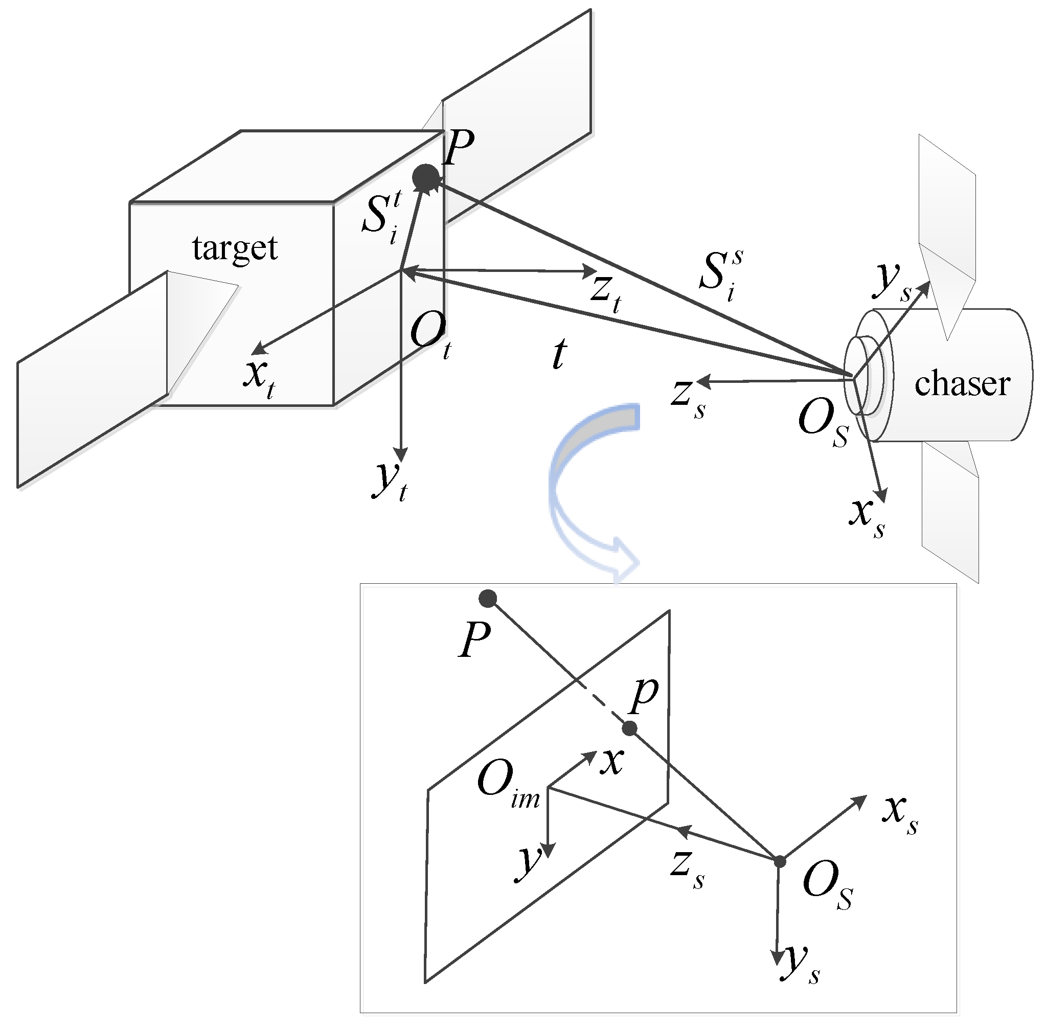
Section 2, we review coordinate systems and the observation model.
Section 3 gives the DOP of the vision-based navigation system in the sensor frame, and
Section 4 gives the quasi-optimal feature point selection method. The performance of the quasi-optimal method is discussed in
Section 5. Finally,
Section 6 is the conclusion.
3. DOP in a Vision-Based Navigation System
In a vision-based navigation system, the geometric distribution of feature points affects the navigation accuracy. The DOP is determined and utilized to estimate the accuracy of the vision-based navigation system.
For
feature points,
is the measurement residual vector with
dimensions and
is the mapping matrix after being linearized with
dimensions. To determine the DOP in a vision-based navigation system, the error of the state vector
should be estimated assuming that
and
are known. The least square method is used to solve Equation (
7), and the error function
is defined as:
where
is a quadratic form and can be expanded as:
Taking the derivative of
with respect to
, we can get:
To get the optimal
, Equation (
10) should be equal to
. Thus, it can be expressed as:
By solving Equation (
11),
is estimated as:
Using Equation (
12), the covariance of the state vector
can be expressed as:
It is assumed that all measurements are independent with the same variance
. The horizontal and vertical variances of a feature point are also assumed to be independent, although they are measured simultaneously. Thus, the variance
can be described as
, and Equation (
13) can be simplified as:
In Equation (
14), the matrix
represents the mapping relationship between the measurement variance and the state error variance.
is a diagonal matrix because of the independence of measurements. Thus, DOP is defined as the sum of the elements along the main diagonal of
with
.
Different from the state vector in the GNSS, which has only the term of position, the state vector of the vision-based navigation system takes position and attitude into consideration. Thus, the DOP of the vision-based navigation system can be divided into PDOP and ADOP, and they are defined as:
Since the DOP of the vision-based navigation system includes PDOP and ADOP, the optimal method for the system searches the subset with the minimum PDOP value or the minimum ADOP value. Subsets with small PDOP values tend to have good geometric distributions. Therefore, they usually have small ADOP values and vice versa.
Equations (
14) and (
15) show that a smaller PDOP (or ADOP) means a higher navigation accuracy of position (or attitude). In GNSS, DOP becomes smaller as the number of satellites increases. It is always true that the PDOP (or ADOP) of the vision-based navigation system will become smaller when more feature points are selected.
4. Quasi-Optimal Method for Selecting Feature Points
A large number of feature points can be extracted from the image. This will result in a large computational load to finish the calculation if all feature points are used. Therefore, it is necessary to select a subset of feature points. The geometric distribution of the feature points on the surface of the target satellite plays a key role in the navigation accuracy. Assuming that feature points are in a plane, this section presents the quasi-optimal method for selecting a subset of feature points.
4.1. The Quasi-Optimal Method
The quasi-optimal method [
24] is initially used to select satellites from different constellations in GNSS. The elements of the matrix
H are the direction cosines of angles between the coordinate axis and vectors from the receiver to satellites. Therefore, the matrix
H is used to select satellites directly. In a vision-based navigation system, the matrix
H has no physical meaning. Thus, other measurements are needed to select feature points.
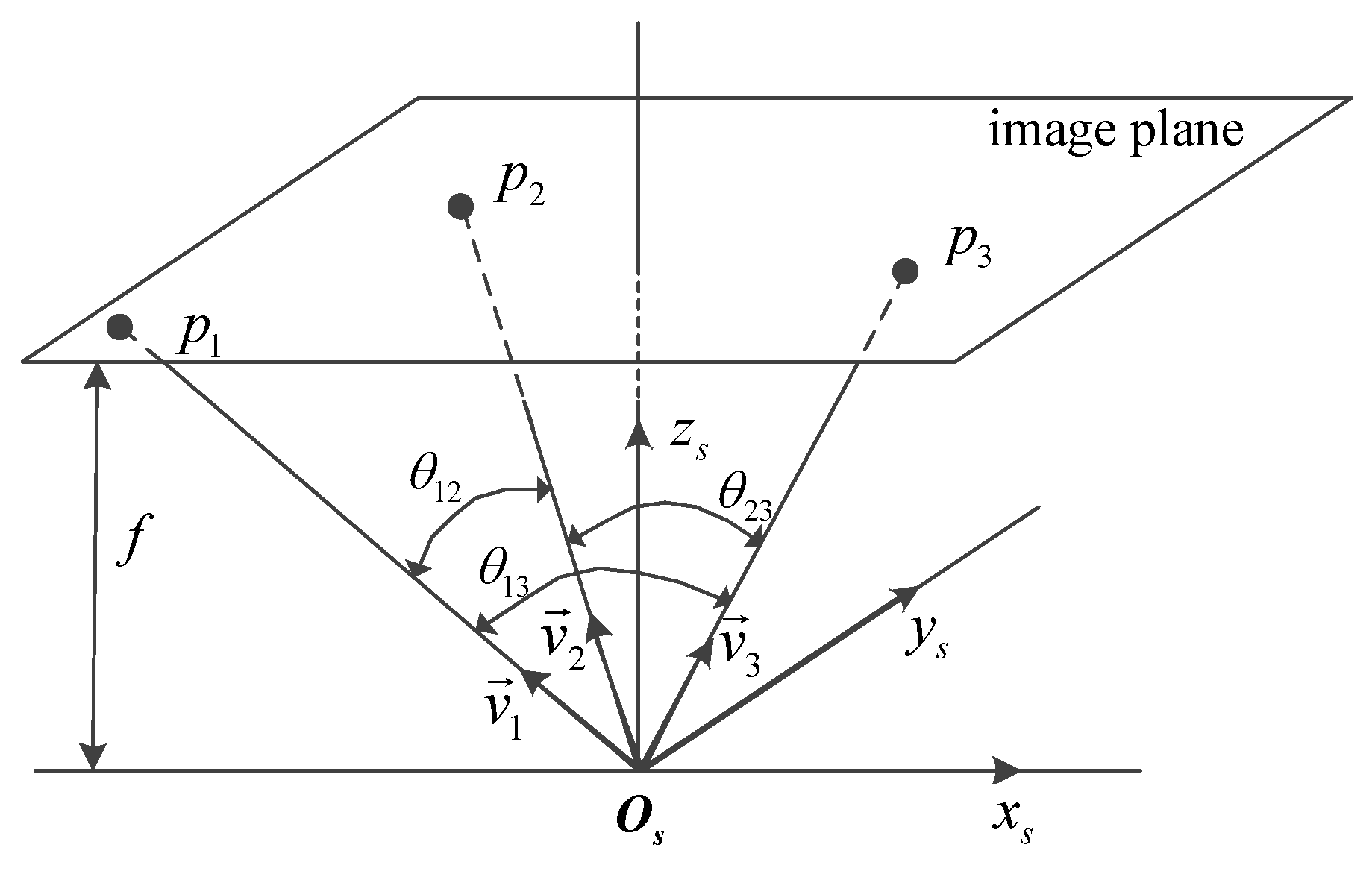
The distribution of the feature points on the image can be described by the angles between the unit vectors from the projection center to feature points as shown in
Figure 2. A small angle between two unit vectors indicates the closeness of the two corresponding feature points on the image.
The cost used in this method is inspired by the intuitive concept that two unit vectors close to each other provide more redundant information. The cost
for the
i-th unit vector and the
j-th unit vector is defined as:
where
is the angle between the
i-th unit vector and the
j-th unit vector.
The cost is a function of the angle between two unit vectors. If the angle between two unit vectors is small or the corresponding two feature points on the image are close to each other, the cost will be large. Otherwise, the cost will be small. The redundancy of the
i-th unit vector can be defined as the sum of costs between the
i-th unit vector and the other unit vectors. It can be described as:
where
n is the number of the total feature points. Equation (
17) represents the redundancy degree of the
i-th unit vector. Redundancies of other unit vectors can be determined in the same way.
For the
i-th feature point, its unit vector is represented as
. Thus,
represents the unit vectors of
n feature points. It is an
matrix, and the matrix
can be calculated as:
where the element of
,
, is the cosine of the angle between the
i-th unit vector and the
j-th unit vector. With Equation (
18), the redundancy of the
i-th unit vector can be rewritten as:
where the superscript 1 indicates that the redundancy lies in initial redundancies.
The redundancy of the
i-th unit vector can be expressed in terms of the sum of the squares of all elements in the
i-th row of the matrix
. All redundancies can be calculated, and the unit vector with largest redundancy can be determined as:
where the subscript
represents the index of the feature point with the largest redundancy.
The feature point should be removed because it provides the least additional information. The -th row and the -th column are deleted from the matrix , and a new matrix with dimensions is generated.
Then, new redundancies and the largest redundancy
are recalculated for the new matrix
using Equation (
21). Remove the
-th feature point, and delete the
-th row and column from the new
. Another new matrix
with
dimensions is generated.
In order to reduce the computational load, Equation (
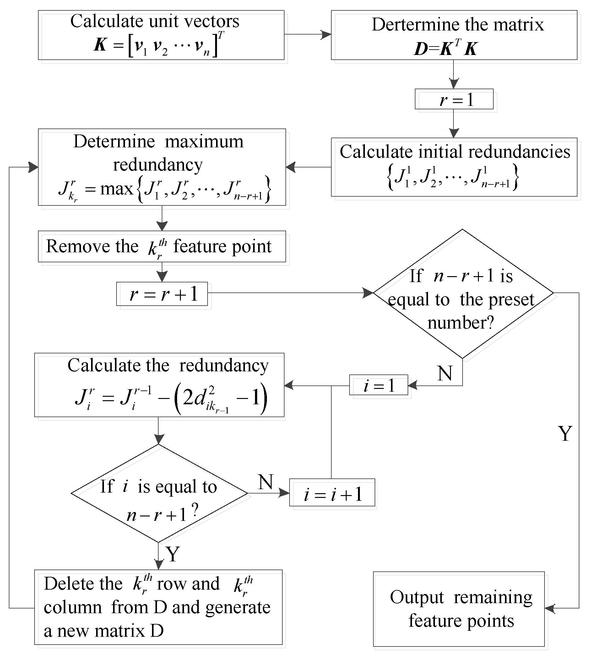
22) is used to compute new redundancies by subtracting the costs of the previous redundancies associated with the removed feature point.
Repeat the procedures above until the number of remaining feature points is the same as the preset number. The flowchart of the method is shown in
Figure 3.
4.2. Analysis of the Method
The quasi-optimal method proposed in this paper is an iterative method that removes the most redundant feature points one by one. An alternative to the quasi-optimal method is the one-step method. This method calculates the initial redundancies firstly. Then, it removes multiple feature points with larger redundancies directly, and the remaining feature points are the selection result.
The feature point with the largest redundancy has different effects on the redundancies of other feature points. Therefore, the feature point with the second largest redundancy in the initial redundancies is not usually the most redundant after the feature point with the largest redundancy is removed. The one-step method does not consider this effect, but the iterative method does. This is the reason why the iterative method is chosen in this paper to filter out feature points. To demonstrate the advantage of the iterative method, an example for selecting two from four feature points is given.
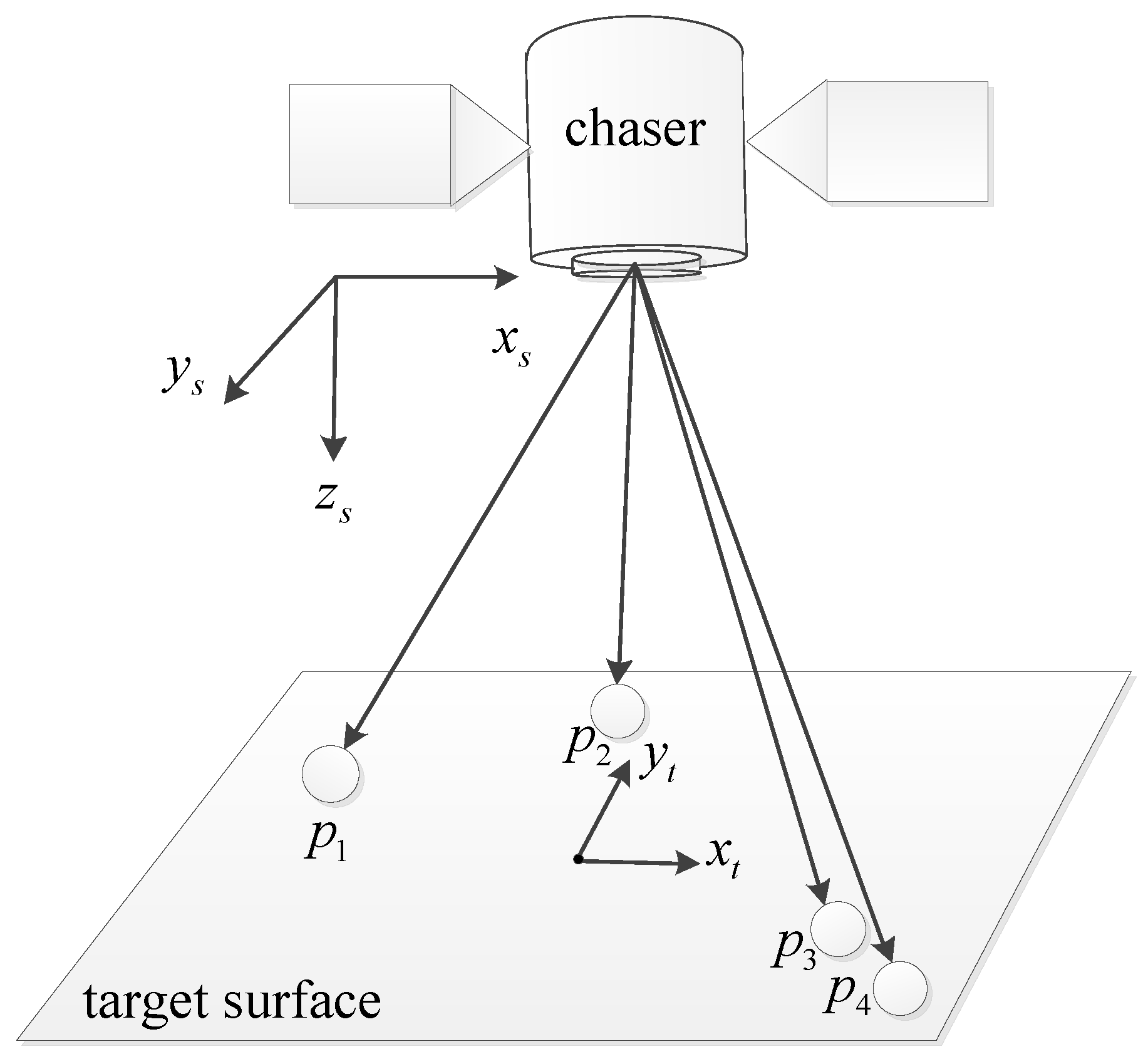
In this example, it is assumed that only translation motion between the target satellite and the chaser satellite exists. There are four feature points on the surface of the target satellite, as shown in
Figure 4, and two of them with a low PDOP value will be selected. The initial condition for this example is shown in
Table 1. Coordinates of the four feature points are in the target body frame.
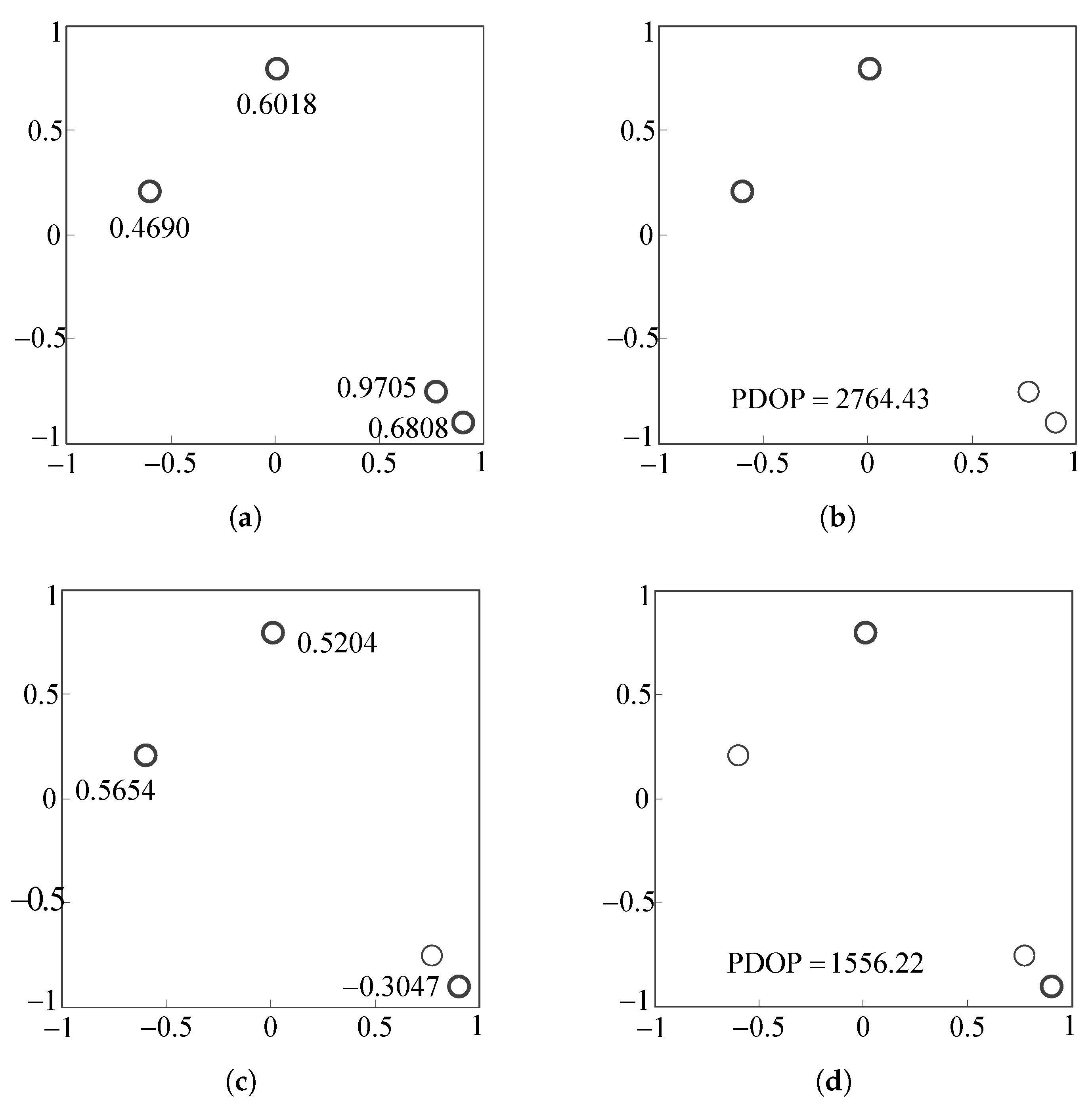
Before removing feature points, the redundancies of the four feature points should be calculated first. The redundancies of
and
are larger than those of
and
, as shown in
Figure 5a. The one-step method is shown in
Figure 5b. It removes the two feature points
and
directly because they have larger redundancies. The PDOP value of the remaining feature points,
and
, is
, which is approximately
-times greater than the optimal PDOP
, as shown in
Table 2.
Figure 5c is the first step of the iterative method. It removes the feature point
and recalculates the new redundancies of the remaining three feature points. Then, the feature point
is removed because it has the largest redundancy in new redundancies as shown
Figure 5d. The two feature points
and
are left. Their PDOP is
, which is only
higher than the optimal PDOP value.
In this example, the iterative method shows a better performance than the one-step method. As shown in
Table 2, the angle between the unit vectors of
and
is only
degrees. Its cost is
, which is much larger than others. Thus, the redundancies of
and
may be larger than those of the others because of the existence of the cost
. When
is removed, the cost
does not exist, and the redundancy of
is lower than the redundancy of others.
5. Simulation and Result
In order to verify the performance of the feature point selection method in the vision-based navigation system, the quasi-optimal method is compared with the optimal method in terms of accuracy and computation time in this section. Due to the significantly increase of the possible combinations, the optimal method could not be completed if the number of the total feature points is large. Therefore, the number of feature points in this section is small.
Simulations in this section are conducted with MATLAB running on a computer with
GHZ Intel(R) Core(TM)2 CPU and 4 GB RAM. Feature points used in simulations are generated by MATLAB randomly in a 1 m × 1 m square plane. Then, coordinates of these feature points in the sensor frame are determined utilizing the coordinate transformation. Using the pinhole model, feature points are projected on the image. The simulation condition is shown in
Table 3.
5.1. Accuracy Evaluation
DOP values are used to evaluate the accuracy of the relative position and attitude with the selected feature points. For better analysis, DOP ratios are used to evaluate the performance. The DOP ratios,
and
, are defined as:
where subscripts
quasi and
optimal represent the DOP values of the quasi-optimal method and the optimal method.
Since the optimal method provides the smallest PDOP and ADOP values in all possible combinations, and are always greater than or equal to one. The closer and to one, the better the geometric distribution of feature points is.
5.1.1. Simulations for Different Total Numbers
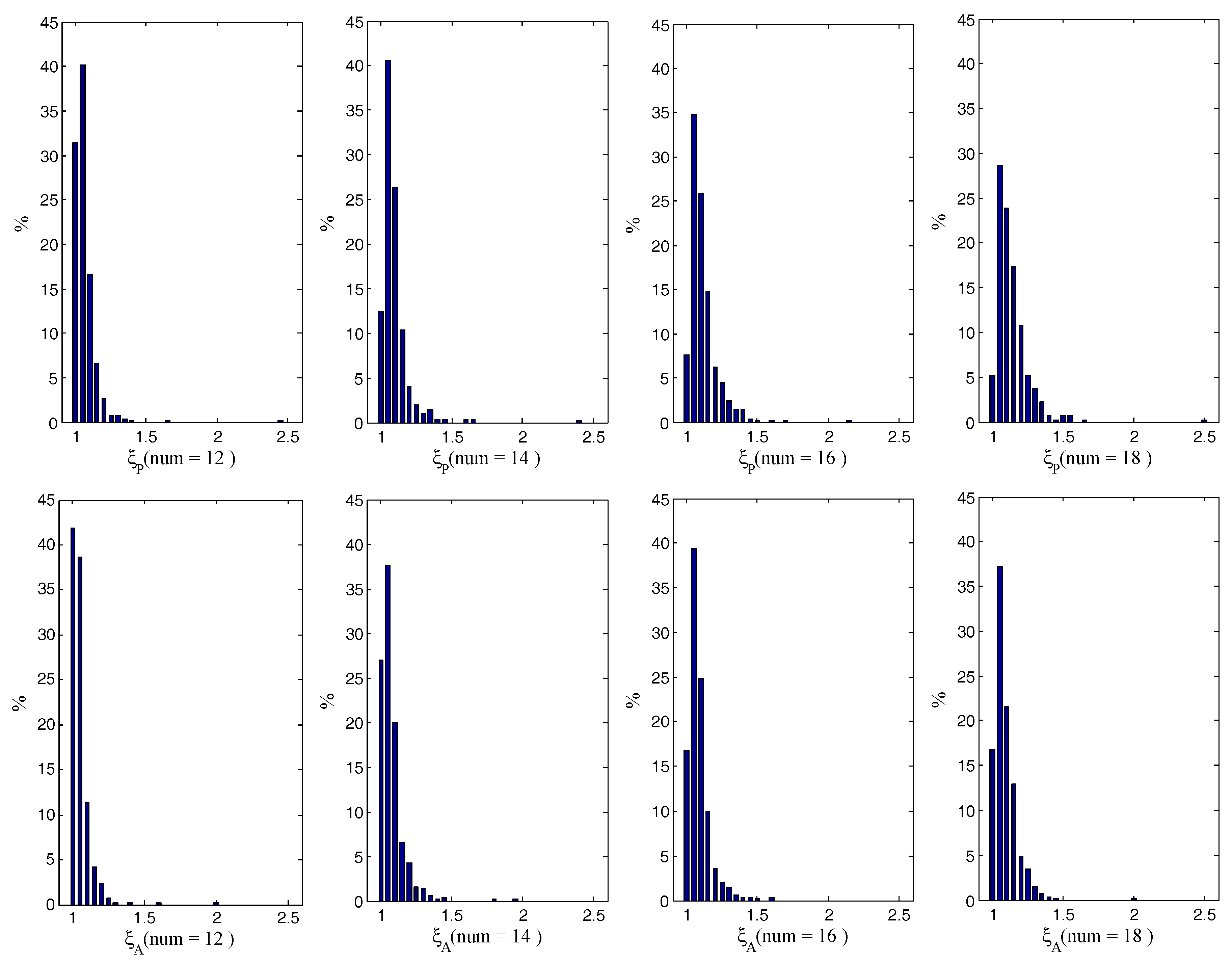
The simulations assume that there are four groups of feature points with different numbers (12, 14, 16 and 18), but only eight feature points are selected. In each group, feature points for 1000 cases are randomly generated. The two selection methods are implemented and tested with these feature points. For each case, the PDOP and ADOP values of the feature points selected by the quasi-optimal method are calculated. The smallest PDOP and ADOP values are selected from all possible PDOP and ADOP values. Then, the DOP ratios, and , are determined and evaluated.
The distributions of
and
for 1000 cases are evaluated in
Figure 6 when the numbers of feature points are 12, 14, 16 and 18, respectively. The bin size is
. It can been seen that the DOP ratios are near one, and most of them are less than
. There are cases with PDOP ratios between 2 and 2.5 and ADOP ratios near two in the four groups. Although, the DOP ratios in these cases are a little large for navigation, this is acceptable because large DOP ratios account for an extremely low percentage.
The average and maximum DOP ratios for different numbers are shown in
Table 4. In the group of 18 feature points, the average
and
are
and
, respectively. Thus, the average PDOP value of the quasi-optimal method is 13.24% greater than the optimal PDOP value, and the average ADOP value of the quasi-optimal method is only 8.97% greater than the optimal ADOP value on average in this group. This indicates that the average PDOP and ADOP values of the selected feature points are close to the average optimal values. Moreover, the other groups perform better than this group on average values.
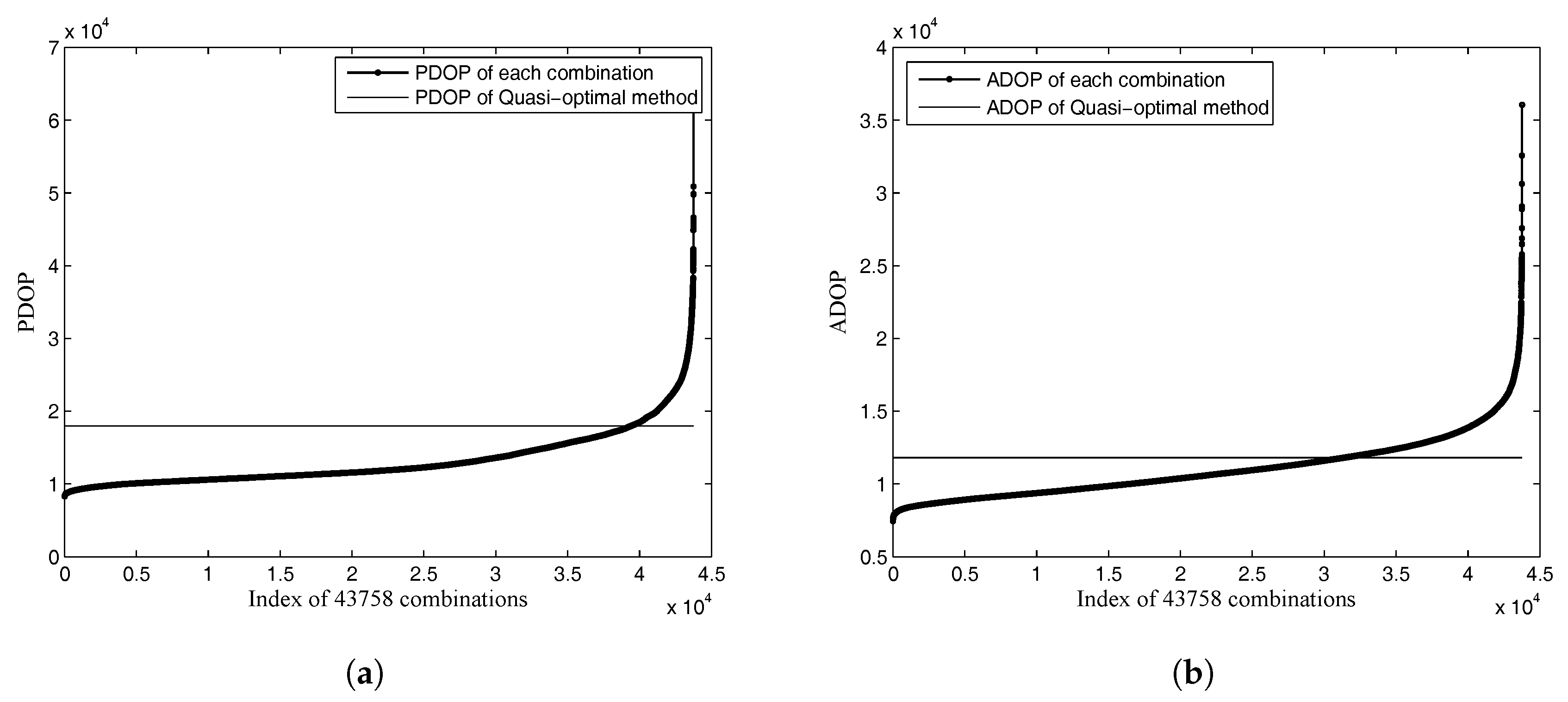
Two cases in the group of 18 feature points are used to analyze the DOP values in worst cases. The
and
of the two cases are
and
, respectively. They are maximum ratios in 1000 cases, as shown in
Table 4. The DOP values of the quasi-optimal method and all possible DOP values are shown in
Figure 7. There are 43,758 combinations, and all possible DOP values are sorted in ascending order. This shows that the PDOP and ADOP values of the quasi-optimal method in the two worst cases are not significantly large compared with those of all possible combinations.
5.1.2. Simulations for Different Selected Numbers
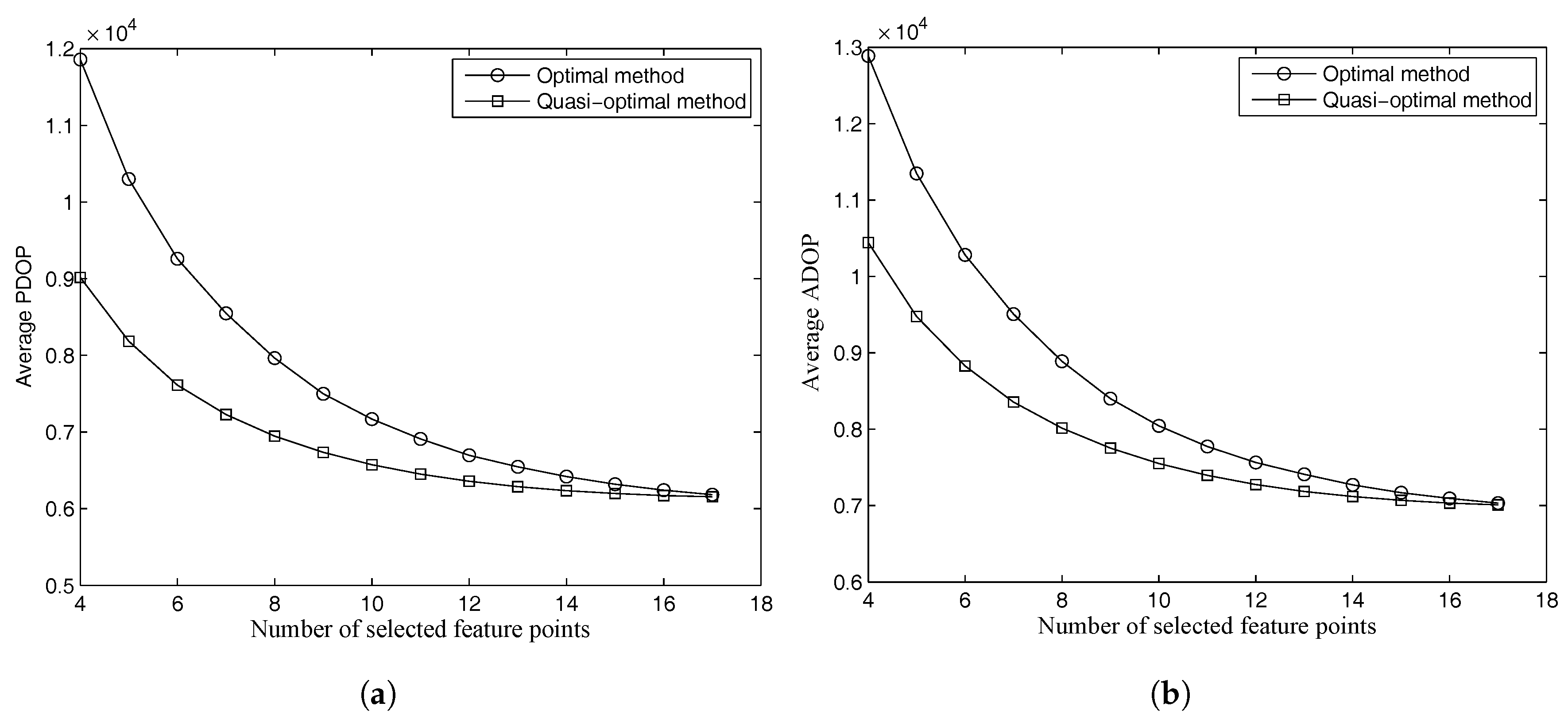
To further evaluate the accuracy of the quasi-optimal method, the two methods are implemented in 1000 cases with 18 feature points. In this simulation, the number of selected feature points is assigned from 4–17 because it takes at least four feature points in a plane to make a nonsingular matrix.
As shown in
Figure 8, the DOP values of the two methods have a similar trend. The figure shows that the mathematical proof derived by Yarlagadda [
29] for DOP in GNSS also works in a vision-based navigation system. The proof indicates that the DOP value decreases as the number of the selected measurements increases. The DOP values of the selected feature points approach those of all feature points when the number of selected feature points increases.
The average PDOP values decrease, and the ratios of the PDOP values given by the two methods to those of all feature points on average are shown in
Table 5. The average PDOP value is flat if the decrease is less than 5%. As shown in
Table 5, the PDOP value of the optimal method is flat when the number of selected feature points is eight. However, the quasi-optimal method requires more than 10 feature points to make the average PDOP value flat. The PDOP value of the optimal method is
bigger than that of all feature points when the selected number is nine. The quasi-optimal method can reach goodaccuracy only when the number is more than 11. This indicates that the position accuracy of the selected feature points is a little lower than that of all feature points with a reasonable selected number. The optimal method performs better than the quasi-optimal method. However, the quasi-optimal method can also perform well by adding the selected feature points. The same result can be obtained for ADOP or the attitude accuracy according to
Table 6.
5.2. Time Performance
The average computation time of the optimal method and that of the quasi-optimal method are estimated in this section. The two methods are used to select 4–8 feature points out of 9–18 feature points for 1000 cases.
Figure 9 shows the average time of the optimal method. The average time of the optimal method increases along with the increasing of the number of the total feature points. The reason is that more feature points provide more possible combinations.
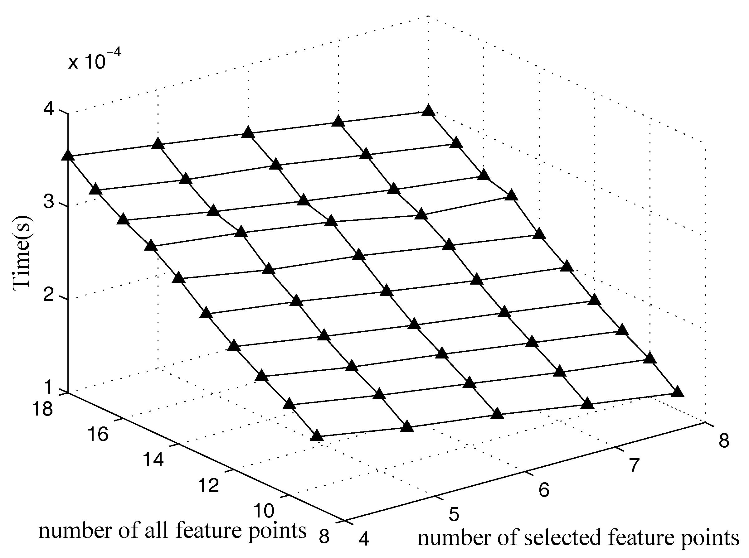
Figure 10 is the average time of the quasi-optimal method proposed in this paper. It shows that the time of the quasi-optimal method increases as the number of feature points increases. Notice that the time of the quasi-optimal is four orders of magnitude lower than that of the optimal method. This means that the quasi-optimal method outperforms the optimal method greatly in terms of computation time.
6. Conclusions
Relative navigation based on vision sensors increasingly becomes significant because of the advantage of accuracy. However, too many feature points on the surface of a target satellite will result in a large computational load and burden the chaser satellite. The main purpose of this paper is to provide an effective method to select feature points.
This paper proposes a quasi-optimal method for selecting a subset of feature points with a good geometric distribution. The method is an iterative method. Firstly, the initial redundancies are calculated, and the feature point with the largest redundancy is removed. Then, the redundancies of the remaining feature points are recalculated, and the second feature point is removed. Feature points are removed one by one through the procedures above until the desired number is reached. Moreover, the dilution of precision is used to verify the performance of the quasi-optimal method. Simulations show that the quasi-optimal method can select feature points with good geometric distribution. Although cases with large PDOP or ADOP values exist, they only account for an extremely low percentage. The results also show that the quasi-optimal method can perform well by adding the selected feature points and requires only a limited time for computation.


