Average Accumulative Based Time Variant Model for Early Diagnosis and Prognosis of Slowly Varying Faults


1
School of Computer and Information Engineering, Henan University, Kaifeng 475004, China
2
Department of Electrical Engineering, Yeungnam University, 280 Daehak-Ro, Kyongsan 38541, Korea
3
School of Automatic, Hangzhou Dianzi University, Hangzhou 310018, China
*
Authors to whom correspondence should be addressed.
Sensors 2018, 18(6), 1804; https://doi.org/10.3390/s18061804
Submission received: 5 May 2018
/
Revised: 28 May 2018
/
Accepted: 30 May 2018
/
Published: 3 June 2018
(This article belongs to the Special Issue Sensors for Fault Detection)
Abstract
:Early detection of slowly varying small faults is an essential step for fault prognosis. In this paper, we first propose an average accumulative (AA) based time varying principal component analysis (PCA) model for early detection of slowly varying faults. The AA based method can increase the fault size as well as decrease the noise energy. Then, designated component analysis (DCA) is introduced for developing an AA-DCA method to diagnose the root cause of the fault, which is helpful for the operator to make maintenance decisions. Combining the advantage of the cumulative sum (CUSUM) based method and the AA based method, a CUSUM-AA based method is developed to detect faults at earlier times. Finally, the remaining useful life (RUL) prediction model with error correction is established by nonlinear fitting. Once online fault size defined by detection statistics is obtained by an early diagnosis algorithm, real-time RUL prediction can be directly estimated without extra recursive regression.
1. Introduction
Abnormal monitoring and efficient tolerant control of large scale systems is significant and crucial since it can guarantee safety and economic production [1,2,3,4,5,6,7,8,9,10,11,12]. For that reason, system abnormal monitoring has received much attention in theoretical and application research areas [1,2,3,4,5,6,7,8]. In general, three steps are required to secure the safety and economic production: abnormal detection, fault pattern recognition, and fault prognosis [1,2]. The first two steps are the necessary means to secure safe production by regular maintenance and repairing at certain time intervals of service time. It can alarm systems abnormal to the operator. Condition-based maintenance is one of the necessary means to secure economic production [2]. However, either abnormal detection or fault pattern recognition can not tell the operator whether a fault will occur and how long will the system be significantly affected, which is the foundation of condition-based maintenance.
Remark 1.
In this paper, “Remaining Useful Life (RUL)” refers to the degrading time between fault- detected points and the point where faults occurred will significantly impact safety or the ability to complete a mission.In addition, the failure time is also defined in statistical means when the fault is statistically significant.
In this section, the existing methods to detect slowly varying faults earlier is firstly overviewed, and then followed with the RUL prediction method overview. The data-driven fault diagnosis method is more applicable in the engineering field since only historical observation data are required, while the precise system model and expert knowledge of the system are not available [8,13,14,15,16,17,18,19,20,21,22,23,24,25]. Machine learning and statistical feature extraction based methods are the most common used ones of data driven fault diagnosis methods. Artificial neural network (ANN) and support vector machine (SVM) are the representative machine learning methods used in fault diagnosis [15,26,27]. However, a large number of historical faulty observations are required to establish a learning modeling of fault diagnosis, and it can not avoid the local optimal problem caused by unsuitable initial values. Principal component analysis (PCA) and partial least square (PLS) are the representative multivariate statistical methods used in data driven fault diagnosis [8,13,14,15,17,18,19,20,21,22]. These methods are more popular since only normal historical observation is required to establish PCA or PLS based abnormal detection models. However, the pattern compounding effect of PCA makes it difficult to diagnose the root cause of the fault. Designated component analysis (DCA) projects the observation to a designated pattern defined by the fault-symptom relation, so it can determine which failure component causes the abnormality [22,27,28]. These data-driven fault diagnosis methods have been widely used in the engineering field. If they are combined with data-driven RUL prediction technologies, fault prognosis approaches without physical models are developed [19,29,30]. Traditional fault diagnosis can only detect the failure moment of the system. For the purpose of fault prognosis, it is expected to detect fault trends as early as possible, and we call it early fault detection. Early detection of slowly varying small faults is an essential step to develop an efficient fault prognosis method [2,29,30].
Remark 2.
In this paper, “failure moment” refers to the point when system is significantly affected by the fault occurring.
Existing early detection methods of slowly varying small faults can be categorized into two classes: model based methods and data-driven methods [3,4]. Inaccurate parameters of a physical model can significantly affect the efficiency of model based early detection of small slowly varying faults. For the purpose of developing a data-driven small fault detection method, many necessary techniques have been used, such as a filter-based method, exponential weighted moving average (EWMA) based method and a cumulative sum (CUSUM) based method [23,24,25,26,31,32,33,34,35,36].
Filter based methods include moving average filter, median filter, wavelet transform (WT) filter, Hilbert–Huang transform (HHT), fast Fourier transform (FFT), short time Fourier transform (STFT), etc. [27]. These methods share the similarity that they all increase the signal-to-noise rate (SNR) of the fault signal by only decreasing the energy of the noise without increasing the the fault size. Although many diagnosing methods have been used as the preprocessing method in the case when small faults occurred, most fault diagnosis methods were invalid as long as SNR of the fault signal still does not increase to a larger value because of the insensitivity of these methods to rather small faults.
Traditional multivariate statistical analysis methods use only the current observation without considering the history information. Thus, the traditional control chart is less sensitive to small faults. To overcome this deficiency, both CUSUM and EWMA based methods take the cumulative sum of the fault size in order to increase SNR of the fault signal [26,30,35]. The main idea of CUSUM-PCA follows as: once the statistics value beyond the threshold defined in advance, make the cumulative sum of the fault size defined by the deviation between the statistics value and the threshold, which can be called fault size cumulating. After the CUSUM process, it can be seen that the fault size at the current time is updated by a cumulative fault size based on all fault sizes at previous times, and CUSUM based control chart can be used as an alternative choice of the traditional control chart [26,30]. Different from the CUSUM method, EWMA uses a weighting coefficient in the cumulative sum step [35]. Compared with CUSUM, EWMA can be more sensitive to small faults as long as the weight coefficient is properly selected. However, the weighting coefficient is usually selected by experience, which implies that it is not a universal value for different fault cases in different application areas.
For the RUL prediction stage following the early detection of small slowly varying faults, two kinds of RUL prediction can be generally used: a state space modeling based method and a statistical modeling based method.
For model based RUL prediction, if there is an exact damage precursor determined by experienced experts and the fault size itself is observable, then a damage precursor based RUL prediction method can be used [33,34,35,36,37,38]. However, the accuracy of the precursor greatly affects the prediction error. Furthermore, fault size can not be observed directly. In most cases, it is difficult to establish an appropriate damage precursor. In [38], a defect propagation model depicted in the form of a mechanistic model is used to predict the RUL of bearing [38]. The stiffness model or a crack growth law based physical relationship is adopted to predict the RUL of mechanical machine [19,39,40,41]. These methods share the same shortcomings: (1) physical model of fault propagation is required; (2) fault degradation process can be directly observed. In general, an accurate defect propagation model is difficult to obtain, which can significantly decrease the RUL prediction efficiency.
In the case when the fault propagation model for an exact damage precursor is unavailable, some state space model based prediction methods can be used, such as the Kalman filter based method, the particle filter based method, and the grey model based method [39,40,41,42]. Brown motion with a constant drift can be used as the state space model [43] for RUL prediction. In [44], Wang and Tsui use linear Brownian motion with adaptive drift as the physical model for RUL prediction with the assumption of inverse Gaussian distribution. In addition, the Kalman filter is adopted to update the drift of Brownian motion model.The innovation of [44] is that posterior drift previously was incorporated into the estimation of drift coefficient at the current time. For the case when the degradation of the faulty system is nonlinear, Si et al. established a [45,46] nonlinear Brownian motion with adaptive drift to get a more accurate RUL prediction method. However, the RUL prediction methods listed in literature [43,44,45,46] are all two-stage methods. These methods share the same deficiency with other model based methods that an accurate physical model is always unavailable. The reason is that the accuracy of drift coefficient for Brown motion model identification will significantly affect the accuracy of the final RUL prediction. On the other hand, an expert system (ES) based method is usually not a first choice for RUL prediction since ES inference and prediction may result in relatively large deviation when adverse knowledge exists in the actual engineering system [47]. A data-driven approach for RUL prediction has been investigated [38]. It is noted that data-driven techniques such as ANN or PCA can be used to establish a data-driven RUL prediction model when the physical model of system degradation process is inaccurate [38]. Thus, the statistical modeling based method is used in this paper for the case when there is no accurate physical model.
Statistical modeling based methods establish the RUL estimation models by fitting the model to historical data under a statistical model without relying on any physical principle [48]. The basic idea of statistical modeling based method is to use historical observed data and statistical models to estimate the RUL [48,49,50]. In general, statistical modeling based methods can be categorized into two classes: models relying on directly observed state information and those that do not. As is already known, there is usually very little failure data. Thus, it is a good alternative to predict RUL based on directly observed state process. The set-up of the failure threshold is often a decision based on the analysis of historical data or the recommended standards provided by expert. In this paper, the observation is assumed to be Gaussian distribution only to determine the threshold through a hypothesis test of some multivariate statistical analysis method. The common used RUL prediction model includes regression-based models, Gamma processes based models, machine learning based models, etc. Regression-based methods establish a regression model for performance parameters first, and then future performance parameters can be predicted by the established regression model autoregressive (AR) or vector autoregressive (VAR) based method, and the time series analysis based method [42,51,52,53,54]. Furthermore, a wide variety of advanced computational techniques such as SVM, ANN, and dynamic Bayesian networks have been used for estimating RUL of industrial systems [42]. ANN based RUL prediction models require a large number of fault degradation signals, which is usually impractical, even when the acceleration life test is used. Moreover, the problem of local optimal can not be avoided. Even fewer fault data are required for SVM to learn a prediction model, and more than one set of faults is necessary.
In the case when only one set of fault data is available, a statistical prediction model such as AR or VAR can be used to predict the fault size in the future [19,30,37]. RUL prediction results based on AR or VAR can only predict impending failure in limited steps ahead [19,30], which does not coincide with the intention of predicting the failure time as early as possible to provide sufficient time for maintenance decision-making. To overcome these limitations, prediction based on multi-step regressive regression is required to estimate the RUL [19]. Due to uncertainty propagation, accumulated prediction error may be a large value during the recursive regression process. In addition, two steps of fault prediction followed by RUL estimation does not coincide with real-time requirements of online prognosis. Finally, a prediction model based on PCA feature extraction can only predict RUL of the system rather than RUL of a specific component of the system.
The main innovations of this paper are as follows: since early diagnosis of slowly varying faults is the fundamental basis of RUL prediction, a more effective AA based time variant model for early fault detection is proposed in the first part of the paper, which can accumulate the fault size as well as decrease the noise of the observation. By using this method, variance of the statistics is much smaller, which is more advantageous for combining a AA based method with a CUSUM based method for detecting fault trends earlier. Then, for the purpose of telling the maintenance department which component should be maintained, RUL prediction for specific components based on the cumulative sum-accumulated average-designated component analysis (CUSUM-AA-DCA) method is further developed. Finally, to illustrate the final goal of early fault diagnosis, the RUL prediction model of exponential regression with error correction is established by nonlinear fitting in the case when early fault trends are diagnosed. The statistics value to describe the performance index and RUL are the independent variable and the dependent variable of the RUL prediction model, respectively. Once the online detection statistics is obtained by an early detection algorithm, the real-time RUL can be predicted by this model without extra multi-step recursive regression.
This paper is organized as follows: Section 2 reviews PCA and DCA based fault detection methods. In Section 3, AA based early diagnosis methods for slowly varying small faults are proposed. In Section 4, an RUL prediction model with error correction is proposed by nonlinear fitting. Section 5 illustrates the numerical simulation of our proposed algorithm to show its efficiency. Section 6 provides the conclusions of this work.
2. Review of PCA and DCA
2.1. PCA
In the case when m sensors are equipped in the system and n observation samples of each sensor are collected, is used to represent the historical normal observation. The following equation illustrates the PCA decomposition of
where is the loading vector defined by eigenvector of , is the ith score vector, is the first columns of the loading matrix, and is the number of key principal components, and is the corresponding residual matrix.
Once the square prediction error (SPE) statistics defined in Equation (2) go beyond the control limit, the system is inferred to be abnormal in the sense of the hypothesis test:
2.2. DCA
The pattern compounding effect of PCA actually makes it difficult to distinguish fault patterns corresponding to a specific component, thus it may fail to reach any practical diagnostic conclusion that the engineer operator required [27,28]. Although a fault pattern recognizing method can be used after detection, diagnosis results by this two step method may be not in real time. Thus, timely fault maintenance strategy can not be made, which may lead to disastrous accidents.
As is already known, PCA projects observation to the loading vector defined by the historical normal data. Different from PCA, DCA projects observation to the designated patterns defined as below:
where
Compute the designated components (DC) via the following equation
where is the designated component vector corresponding to .
Similar to PCA, DCA decomposition of can be described in Equation (7) [22,27]:
where is the number of designated patterns.
A hypothesis test of normal distribution can be used as a tool to determine the control limit of each designated component.
Remark 3.
The designated pattern can be defined by experts’ experience or by machine learning to a specific faulty observation.
3. AA Based Early Diagnosis of Slowly Varying Small Faults
An early detection method is necessary not only to detect the fault occurring moment, but also to predict the RUL of the system before it is broken down. In this part, an AA technique is proposed to increase the fault size as well as to decrease the noise energy, thus SNR of the fault signal can be significantly enhanced, which is beneficial for early detection of slowly varying faults.
3.1. AA Based Time Variant PCA for Early Abnormal Detection
As stated in Section 1, the CUSUM based method uses the cumulative sum of fault size to enhance the SNR of the fault signal. In the case when fault size can not be directly observed, statistics of PCA such as SPE can be defined as an indirect fault size to be cumulated in CUSUM-PCA [25]. However, it does not take noise energy decreasing into consideration, so the efficiency of early abnormal detection is not satisfactory.
In this subsection, with our intention to decrease the noise variance of the observation as well as to cumulate the fault size at each sample time, a new AA based time variant PCA model is proposed for early detection of fault evolved slowly.
Remark 4.
It can be proved that, after the AA process, the noise variance of the observation can be decreased as well as the fault size can be increased. On the other hand, the average accumulative observation at each time is not identical independent distribution (i.i.d.) samples any more. To overcome this limitation, time variant AA model can be established as long as there is adequate number of historical normal data.
The detailed algorithm includes seven steps:
A. Offline modeling
Step 1: Assume there are samples of normal historical observation. Denote as the stacked normal historical observation, where m is the number of observation variables involved in the system, n is the number of samples of each variable, and N is equal to the number of samples of online observation.
Step 2: Compute N set of average accumulation from
where is the element of , is the element of , and the superscript denotes the kth set of average accumulative observation.
Step 3: Establish N anomaly detection models based on each from
where is the first columns of the loading matrix, is the number of key principal components for the kth PCA model, is the score matrix, and is the residual matrix.
Step 4: The statistics of SPE are used for anomaly detection. The control limit can be determined by
where
is the -quantile of normal distribution , and is the eigenvalue of .
B. Online detection
For online detection, it is assumed that the online data is defined as
where is the online normal observation of the jth variable at sample time i, and is the observation variation of the jth variable at sample time i when the system is abnormal.
Online early fault detection of slowly varying small faults follows as Steps 5–7:
Step 5: Compute the average accumulative sum of the previous k samples from
where
The signal-to-noise-rate (SNR) of is defined as
where is the noise variance of .
Remark 5.
It should be noted that the fault signal is assumed to be a deterministic signal generated by performance degradation of a component in the system.
After average accumulative summing, it can be proved that
where is the SNR of which is defined as
The detailed proof is as follows:
where and , denotes the variance operation of x.
Since the noise variance decreases times, we can prove that as long as .
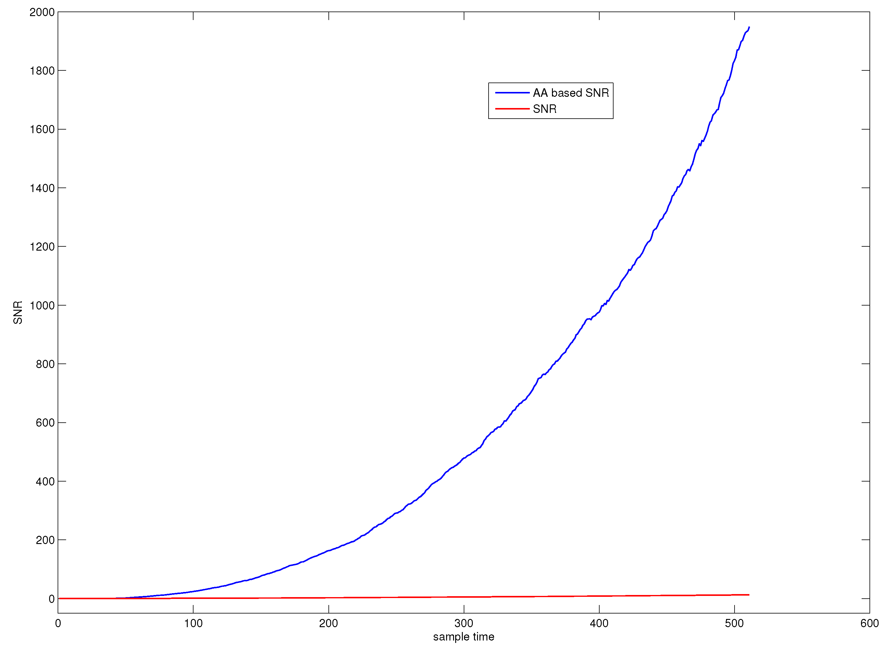
Figure 1 illustrates the SNR of a fault observation, where the red line represents the original SNR and the blue line represents the SNR computed by average accumulation. The figure indicates that average accumulative technique can greatly enhance the SNR of the small slowly varying fault buried in noise.
Remark 6.
The key idea of small fault detection is to increase the fault size and to decrease the noise energy. In such a way, the control limit can be decreased and the fault size can be increased.
Step 6: Project to the principal model defined in Equations (9) and (10). Compute the online SPE value from
where is the residual vector when is projected to the principal component space spanned by .
Step 7: If violates the control limit of the kth principal model, the system is abnormal at time k; otherwise, the system is normal.
3.2. AA Based Time Variant DCA for Early Fault Diagnosis
AA-PCA can be used for early detection of slowly varying faults, but it is only efficient in early detection of system abnormality. The pattern compounding effect of PCA makes it difficult to recognize which component failure is the root cause [27,28]. In general, root causes of different faults correspond to different components of the system. Especially, in the case when multiple faults are involved in the system, each fault may occur from different times. On the other hand, fault prognosis is in essence the RUL estimation of every component, which can tell the engineering operator how long a specific component will be maintained or replaced. Thus, early separate diagnosis of every slowly varying fault component is required for fault prognosis. In this subsection, an average accumulative based time variant DCA model for early diagnosis is proposed.
The algorithm includes the following five steps:
A. Offline modeling
Step 1: Obtain N sets of average accumulation of historical observation from Equation (8).
Step 2: Project the average accumulated historical data to the designated pattern defined in advance according to the fault-symptom knowledge determined by experts or data driven machine learning algorithms:
Step 3: Establish N DCA fault diagnosis models.
Since is still normally distributed with zero mean, a designated component of normal observation should be located in the confidence interval of with the confidence level , where is the variance of . The control limit for fault diagnosis can be computed by hypothesis testing via the following equations:
B. Online early diagnosis for slowly varying small faults
Step 4: Project the average accumulated online data to the designated pattern , where k is the current sampling time:
Step 5: Comparing with the control limit of the kth DCA fault diagnosis model to evaluate whether the fault corresponding to has occurred in the system.
Instead of AA-PCA based time variant early fault detection, which can only detect whether the system is abnormal, the AA-DCA based time variant model for early diagnosis can effectively detect which component of the system is failure and the start point of each small fault can also be detected.
3.3. CUSUM-AA Based Early Diagnosis of Slowly Varying Small Faults
Even though the AA based method is efficient for slowly varying fault detection, more early small faults can not be well detected. On the other hand, the variance of the AA based statistics characterizing fault size is much smaller, which is beneficial for combining the AA based method with the CUSUM based method. Combining AA with CUSUM, a novel CUSUM-AA based method is developed in this subsection. It can be seen from Section 3.1 and Section 3.2 that cumulative sum-accumulated average-principle component analysis (CUSUM-AA-PCA) is similar to CUSUM-AA-DCA with the exception that the statistics used are SPE for CUSUM-AA-PCA and DC for CUSUM-AA-DCA, respectively. In order to save space in this paper, only the CUSUM-AA-DCA method for early diagnosis of slowly varying small faults is illustrated in detail. This method aims to diagnose slowly varying small faults earlier than AA-DCA.
There are six steps included in the CUSUM-AA-DCA algorithm:
A. Offline modeling
Step 1: Compute the average accumulation of historical observation via Equation (8).
Step 2: Compute the AA-based designated component from Equation (21).
Step 3: For early fault diagnosis of multiple slowly varying faults occurring at different times, CUSUM-AA based Shewhart control charts incorporating historical information for each DC is used as an alternative choice of traditional Shewhart control charts:
where and are the upper and lower CUSUM designated component statistics, is the mean of , is usually a more tight threshold than that of the traditional method, such as one half of the traditional control limit [30]. It can be seen that the fault size beyond is added in a cumulative manner.
Step 4: Determine threshold as a new control limit of the jth designated component based on CUSUM-AA. The criterion with smallest miss detection rate is used to determine the new control limit. In fact, as long as is properly chosen to ensure the number of samples beyond is small enough, the CUSUM-AA based can be a rather small value. The ideal value of is zero.
B. Online early diagnosis for slowly varying small faults
Step 5: Project to the designated pattern to obtain the average accumulative designated component .
Step 6: Using the same means of cumulative sum with offline modeling to cumulate the online via the following Eqs.:
Step 7: Comparing with the control limit to evaluate whether the fault corresponding to has occurred in the system.
The CUSUM-AA-PCA based early detection method for slowly varying faults can be developed in a similar manner.
4. RUL Prediction
Once the health state of the system is detected online, RUL of the current state should be estimated for decision-making of system maintenance. Here, the RUL prediction model based on historical fault data is established first. Then, online RUL prediction using the RUL prediction model can be obtained.
In this paper, we only consider those slowly varying faults with certain degradation rates.
4.1. Damage Precursor and RUL Prediction Model Based on Historical Fault Data
4.1.1. CUSUM-AA-PCA Based System RUL Prediction Model
For sake of establishing an RUL prediction model, a degradation precursor based on early detection results of CUSUM-AA-PCA to historical faulty observation should be determined in the first step.
Firstly, early detection point of fault trends can be determined by the following criterion:
where is the control limit of CUSUM-AA-PCA model, and the subscript 0 represents the corresponding value of the historical fault observation.
Secondly, the failure point can be determined by the following criterion:
where is the control limit of PCA model established directly from the historical normal observation.
Thirdly, the evolution process between and of the statistics for CUSUM-AA-PCA can be defined as the damage precursor from
Define the RUL at t as
Then, using the damage precursor and the RUL at each , a nonlinear fit curve is developed to establish the rough RUL prediction model as below:
Once SPE is used as a statistics to characterize the damage precursor, exponent function defined in the following equation is adopted to fit the curve of damage precursor:
The prediction model proposed in this subsection can be used for online RUL prediction of the same fault as modeling.
Remark 7.
As is already known, RUL based on accumulated damage usually has the form of exponent function. Since accumulated SPE is used to define fault size, there is no function choice problem because accumulated damage is used.
Model error will inevitably result in online RUL prediction error. Thus, an error correction table can be developed in the modeling stage via the following criterion:
The corrected prediction model can be illustrated as
where is the online SPE value of CUSUM-AA-PCA, and it can be computed in a similar form to Equation (30) by replacing with .
The common used AR or VAR prediction model characterizes the successive linear relation in local range [24]. It can only well predict the fault size in limited steps ahead, called steps. When the failure will come after steps, it can not directly predict the RUL. Multi-step regression in recursive form is required to predict how long the system will be failure. Therefore, the RUL prediction by VAR is not real-time.
Compared with the regression prediction model, the main advantage of our RUL prediction model is as follows:
- (1)
- It can directly predict the RUL without extra recursive regression, thus it can insure ’real-time’ prediction of the RUL.
- (2)
- The model established has the error correction term, so it can come to an accurate prediction.
4.1.2. Online RUL Prediction
Once online is obtained, the RUL at time k can be predicted online as
where is the error correction term when the online statistics value is .
The online error correction term can be determined by the following criteria:
- (1)
- If there is a such that , then
- (2)
- If there is no such that , then
4.2. DCA Based RUL Prediction of Each DC
Different from the ability of PCA to detect system abnormal without finding the root cause of the fault, DCA can diagnose multiple faults well corresponding to different components of the system. On the other hand, the system maintenance engineer wants to know exactly which component should be repaired, so it is more valuable to develop an RUL prediction model based on each DC of CUSUM-AA-DCA.
Replace with to get the starting point and failure point of the fault corresponding to
where is the control limit of the the DC corresponding to .
The failure point can be determined by the following criterion:
where is the upper control limit of DCA model established directly from the historical normal observation.
The damage precursor corresponding to can be computed as follows:
RUL of the component corresponding to at t is defined as
Then, fitting curve of and the RUL at each can be developed as
The corresponding error correction table can also be determined via the following relationship
Once online is obtained, the RUL at time k can be predicted online as
5. Simulation
In this part, we illustrate the numeric simulation analysis of AA based time variant model for early diagnosis and prognosis.
The parameters used are , and . The historical normal observation is generated by the following equation:
where , defined by Equation (4), are the 12 variation patterns to generate observation data, and is the n samples of with the distribution .
In software, MATLAB, the function "randn" is used to generate :
The contributions of the fault pattern corresponding to , , and increase to a large value by
where the fault signal is samples of negative exponential function or linear polynomial function with small slope characterized by
with the parameter value , , and .
It can be easily seen from Equations (63)–(68) that every fault occurs at different times and each has a different degradation rate.
5.1. AA-Based Time Variant Early Detection of Slowly Varying Small Faults
5.1.1. AA-PCA Early Detection
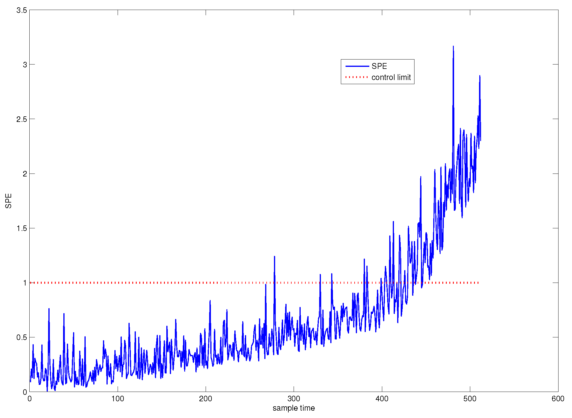
First, traditional PCA is used for system monitoring. The SPE chart of PCA is shown in Figure 3, from which from which it can be seen that the system is abnormal from the 425th sample point. The confidence level we have chosen is , that is to say, the system is abnormal in the sense of very high confidence level. Hence, we call this fault detection point as the system failure point.
On the other hand, we can see from Figure 3 that a slowly varying fault has occurred in the system from a moment much earlier than the failure point. Before the failure point, the fault is not significant enough to be detected.
CUSUM-PCA is one of the most commonly used early detection methods since it can cumulate fault size beyond a tighter threshold.
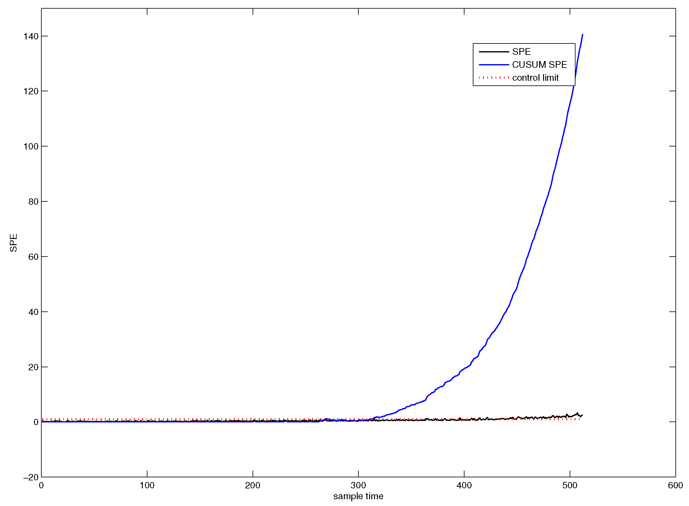
Figure 4 shows the SPE chart for CUSUM-PCA. The blue line denotes the SPE value of CUSUM-PCA, and the black line represents the SPE value of PCA. It can be seen from Figure 4 that the system has followed an abnormal trend from the 311th sample point.
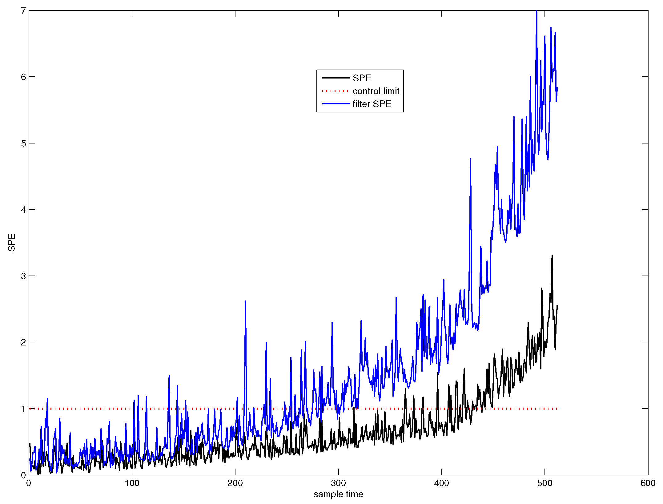
The SPE chart of wavelet filter (WF) based PCA is depicted in Figure 5. The blue line denotes the SPE value of wavelet filter based PCA (WF-PCA), and the black line denotes the SPE value of PCA. It can be seen from Figure 5 that the system has followed an abnormal trend from the 281th sample point.
As we have analyzed in Section 1, either filter based method to decrease noise energy or the CUSUM based method to cumulate the fault size can not detect the fault trend well as early as possible. Figure 6 illustrates the early fault detection result of time variant AA-PCA. It tells us that the fault trend can be detected at the 57th sample point.
It can also be seen from Figure 6 that the fault trend has occurred before the detection point . Since the noise energy has been reduced to a rather small level, so the CUSUM technique can be used for the SPE chart of time variant AA-PCA.
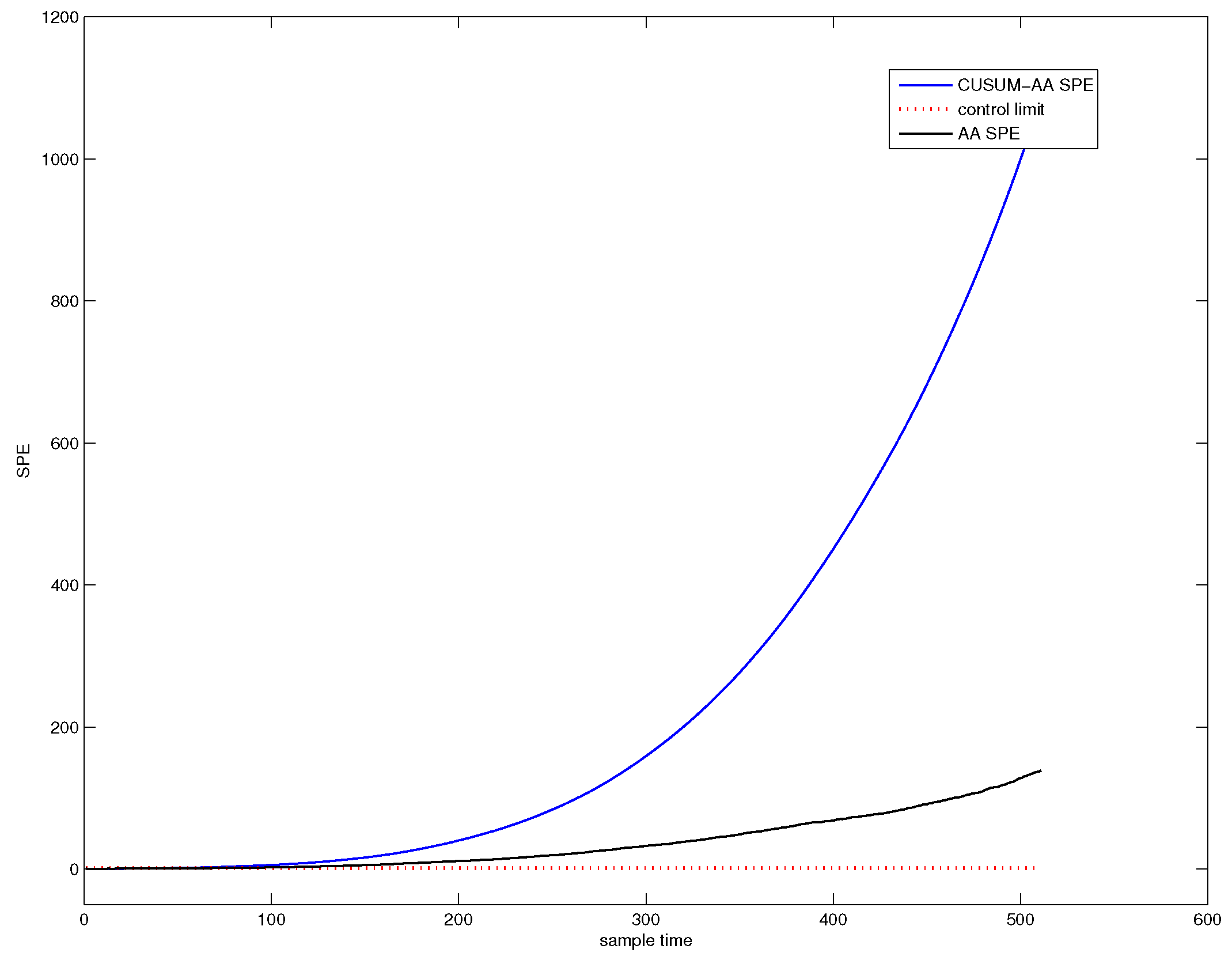
Figure 7 shows the detection efficiency of the CUSUM-AA-PCA method. The blue line denotes the SPE value of CUSUM-AA-PCA, and the black line denotes the SPE value of AA-PCA. Figure 7 indicates that the system has started an abnormal trend from the 44st sample point.
The miss detection rate, false detection rate, and the fault trend detection point corresponding to Figure 3, Figure 4, Figure 5, Figure 6 and Figure 7 are listed in Table 1. From the table, it can be concluded that CUSUM-AA based time variant early fault detection for a slowly varying fault is a more efficient method since it can effectively decrease the noise energy as well as can accumulate the fault size.
5.1.2. AA-DCA Based Early Diagnosis
Affected by the pattern compounding effect, the PCA based fault detection method and its variations can only alert users that the system is abnormal. It can not find the root cause of the fault component. DCA is introduced to overcome this problem. Figure 8 shows the Shewhart chart of AA-DCA diagnosis and DCA diagnosis. The black line represents the Shewhart of DCA diagnosis, the blue line denotes the Shewhart of AA-DCA diagnosis, and the red dotted line are the upper control limit and the lower control limit, respectively.
From Figure 8, it can be seen that three faults corresponding to , , and have occurred in the system. The detection point of each fault is listed in Table 2.
Figure 9 shows the Shewhart chart of CUSUM-AA-DCA diagnosis. The subfigures (a–c) are the Shewhart charts to , , or of CUSUM-AA-DCA. The subfigures (d–f) are the Shewhart charts to , , or of AA-DCA. The dotted red line is the control limit.
From Figure 9, it can be seen that CUMSUM-AA-DCA can diagnose faults at earlier times than that of AA-DCA. The miss detection rate, false detection rate, and the fault trend detection point of different method are listed in Table 2. Comparing the 2nd row, the 6th row and 10th row of Table 2 with the 2nd row of Table 1, it can be concluded that the detection point of the SPE chart for PCA is not equal to any of the detection point of , , or , which implies that PCA can not effectively detect the root cause of the faults.
5.2. Fault Prognosis
In this part, we first use the early fault detection result based respectively on CUSUM-AA-PCA and CUSUM-AA-DCA of the historical fault observation to establish the damage precursor and the RUL prediction model. Then, online RUL can be predicted.
Remark 8.
Although an AA based time variant model is the foundation of this paper, in order to save space in this paper, only CUSUM-AA based RUL prediction is illustrated in this part since CUSUM-AA can detect slowly varying faults at earlier times ahead of failure.
5.2.1. RUL Prediction Model Based on Historical Faulty Observation
For the purpose of establishing an RUL prediction model, a damage precursor characterizing the fault size evolving process should first be determined. In this subsection, the statistics value characterizing fault size is SPE of CUSUM-AA-PCA. Implement PCA into the historical fault observation, and display the SPE chart in Figure 10. Using this control chart to determine the failure point, .
By implementing CUSUM-AA-PCA into the historical fault observation, the corresponding SPE chart can be shown in Figure 11. We can use this chart to determine the starting point .
The obtained SPE value for CUSUM-AA-PCA from to can be defined as the accumulated damage precursor.
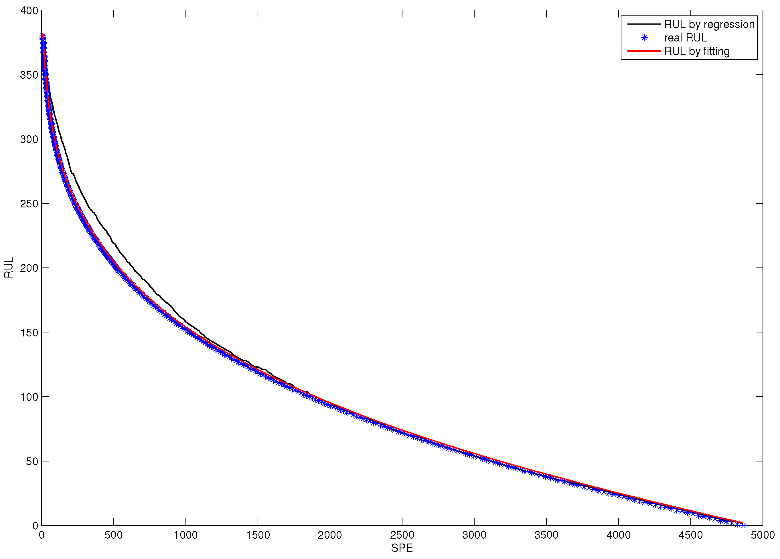
Figure 12 shows the nonlinear fitting curve of the accumulated damage precursor. The blue scatter chart denotes the real historical RUL and the red line denotes fitted RUL.
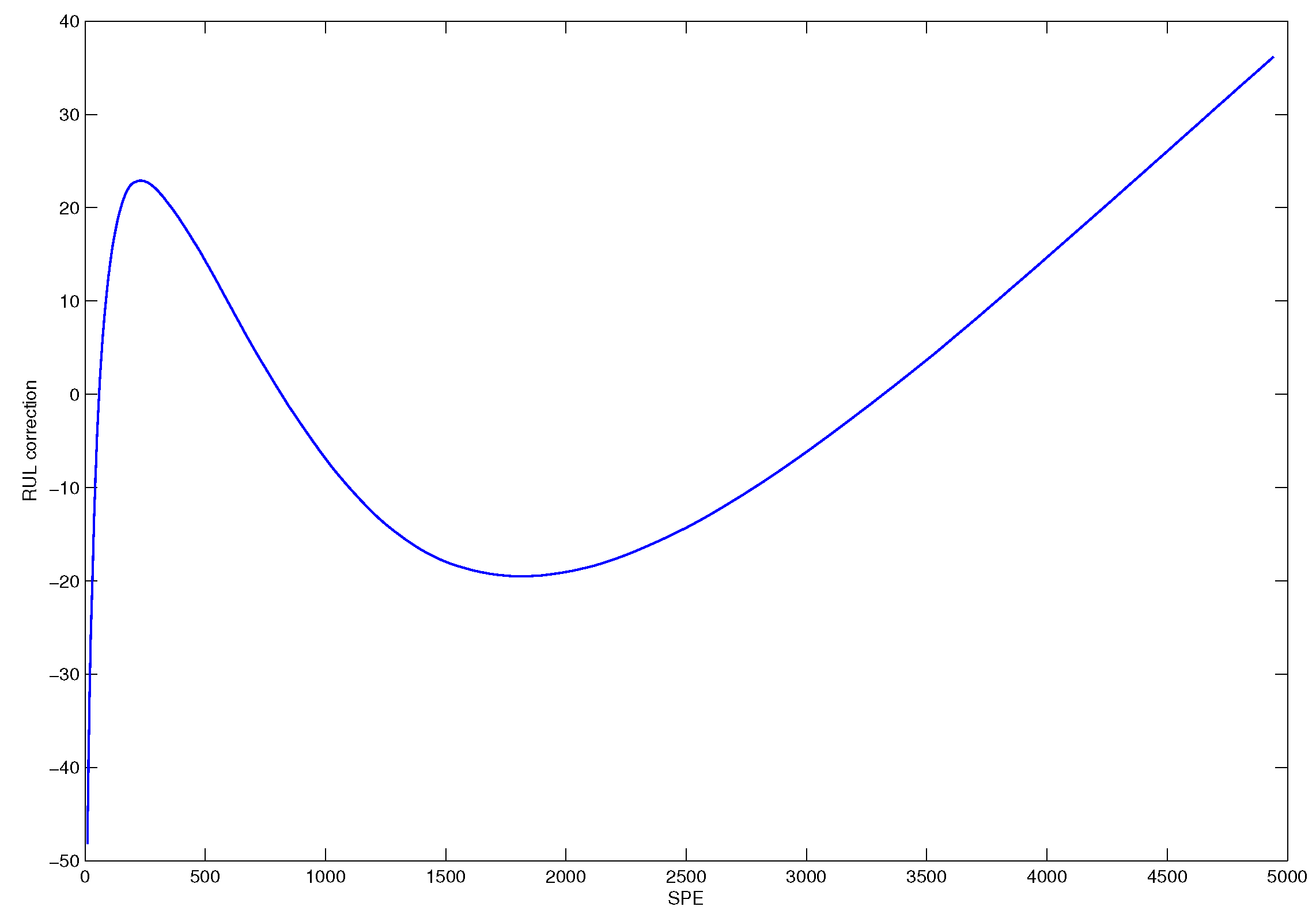
The error correction curve illustrated in Figure 13 can be used to establish a error correction table for the prediction model.
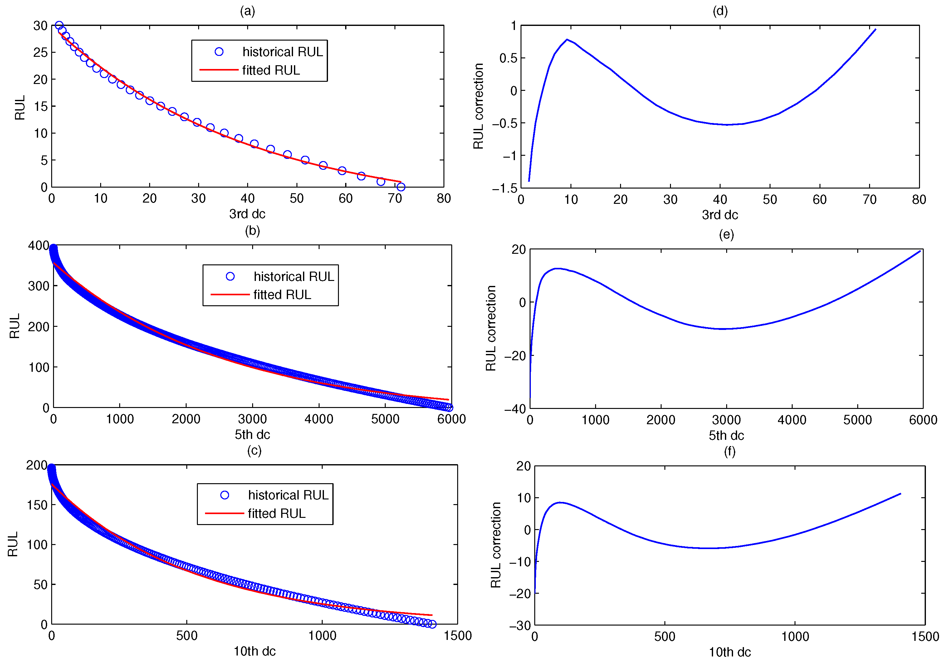
Figure 14 shows the fitted RUL prediction model of CUSUM-AA-DCA. The blue scatter chart denotes the real historical RUL, and the red line denotes fitted RUL. The left part is the fitted RUL prediction model for the three fault patterns corresponding to , , and , and the right part is their model error correction curve.
5.3. Online RUL Prediction
Once online of CUSUM-AA-PCA is obtained, use Equation (38) to predict the online .
Figure 15 shows the online RUL prediction result of the CUSUM-AA-PCA fault prognosis method. The scatter chart denotes the real RUL, the black line represents the rough predicted RUL, and the blue line is the corrected RUL.
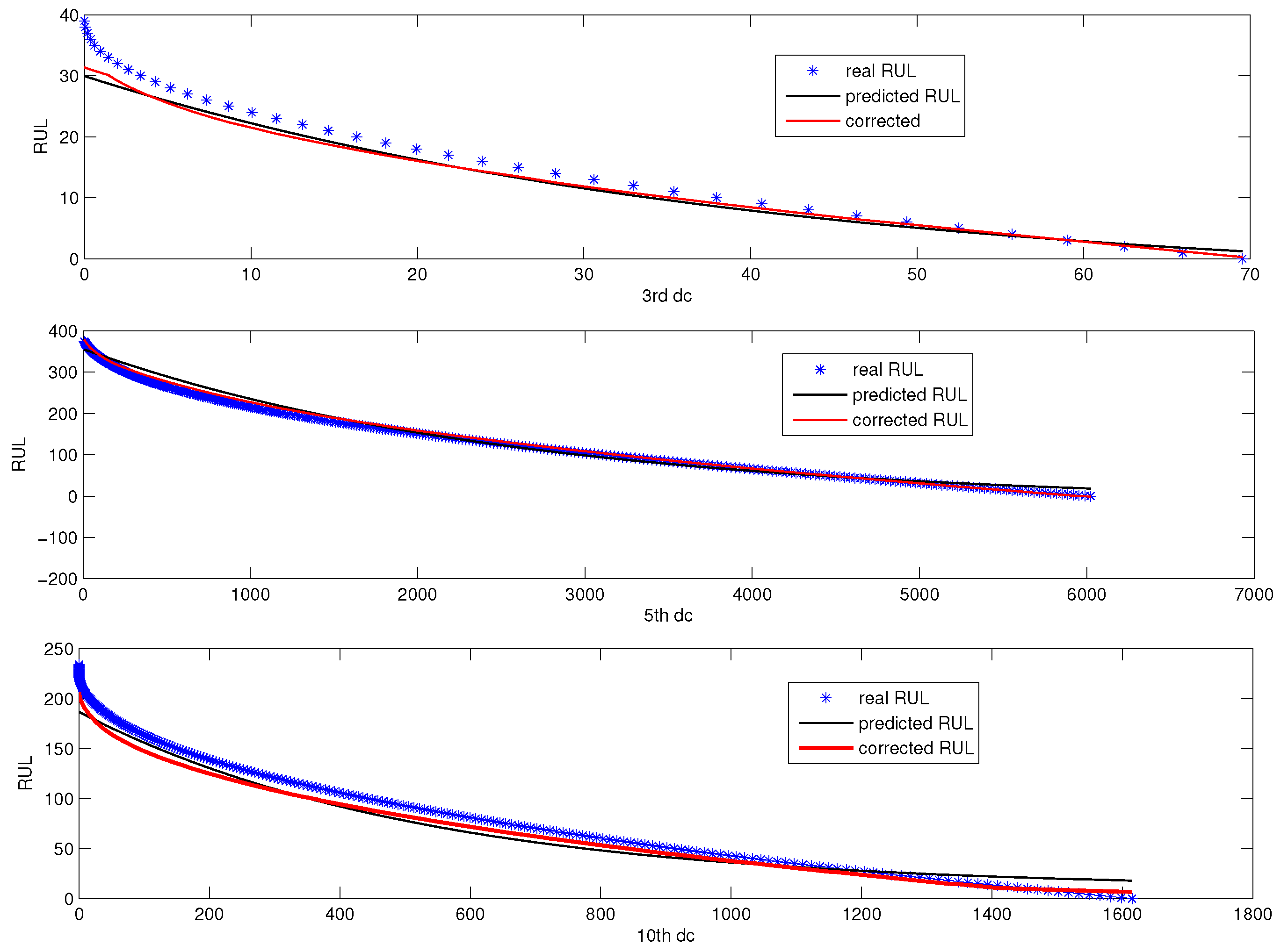
Figure 16 is the online RUL prediction based on the three designated components corresponding to , , and . The scatter chart denotes the real RUL, the black line is the rough predicted RUL, and the blue line is the corrected RUL.
Figure 15 and Figure 16 tell us that the proposed RUL prediction model with error correction is effective for fault prognosis in the sense that RUL prediction error is small. Figure 17 shows the online RUL prediction of AutoRegressive (AR) following recursive RUL estimation. Figure 18 is the RUL prediction using AR to DC corresponding to , , and . It can be seen from Figure 18 that the fitted RUL prediction model with error correction is more efficient than that of the AR model.
The mean of absolute RUL prediction error is listed in Table 3. From Table 3, it can be concluded that the RUL prediction model with error correction is a better choice in the case when only one set of fault observations is available.
Remark 9.
If the variance of the statistics characterizing fault size is larger, the efficiency of the fitted prediction model with error correction will be more superior to that of the AR prediction model. The reason is that the AR prediction model is a local linear model, and error propagation is significant during the recursive regression process.
6. Conclusions
Condition-based maintenance is one of the necessary means to ensure safety and economic production. The purpose of fault prognosis is to judge whether a fault will occur and how long the system will break down in the future, which is the foundation of condition-based maintenance. Early detection of slowly varying fault is an essential step for developing an accurate RUL prediction model.
In this paper, we first propose a novel AA based time variant PCA model for early detection of slowly varying small faults, which can accumulate fault size as well as decrease the noise energy. DCA is introduced to develop an AA based time variant DCA to diagnose the root cause of the fault, which is helpful for the operator to make decisions about system maintenance. Then, the AA based method is combined with the CUSUM based method to detect fault trends at earlier times. Finally, the RUL prediction model with error correction is established by nonlinear fitting. Once the online fault size defined by a detection statistics value is obtained by an early diagnosis algorithm, the online RUL can be predicted by this fitting curve and the error correction table.
In the case of many sets of fault observations being available, deep learning based on early detection and prognosis of slowly varying faults will be our future focus.
Author Contributions
Conceptualization, Funa Zhou and Chenglin Wen; Methodology, Funa Zhou and Ju H. Park; Validation, Po Hu and Funa Zhou; Writing-Review & Editing, Funa Zhou and Ju H. Park; Visualization, Po Hu; Project Administration, Chenglin Wen.
Funding
This research was supported in part by the National Natural Science Foundation of China (Grant No. U1604158, 61333005, U1509203, 61751304 and 61673160).
Conflicts of Interest
The authors declare no conflict of interest.
References
- Cai, J.; Ferdowsi, H.; Sarangapani, J. Model-based fault detection, estimation, and prediction for a class of linear distributed parameter systems. Automatica 2016, 66, 122–131. [Google Scholar] [CrossRef] [Green Version]
- Li, Y.G.; Nilkitsaranont, P. Gas turbine performance prognostic for condition-based maintenance. Appl. Energy 2009, 86, 2152–2161. [Google Scholar] [CrossRef]
- Zhang, N.; Wu, L.; Yang, J.; Guan, Y. Naive Bayes Bearing Fault Diagnosis Based on Enhanced Independence of Data. Sensors 2018, 18, 463. [Google Scholar] [CrossRef] [PubMed]
- Yin, S.; Li, X.; Gao, H.; Kaynak, O. Data-based techniques focused on modern industry: An overview. IEEE Trans. Ind. Electr. 2015, 62, 657–667. [Google Scholar] [CrossRef]
- Zhang, R.; Peng, Z.; Wu, L.; Yao, B.; Guan, Y. Fault Diagnosis from Raw Sensor Data Using Deep Neural Networks Considering Temporal Coherence. Sensors 2017, 17, 549. [Google Scholar] [CrossRef] [PubMed]
- Xu, X.; Li, Z.; Li, G.; Zhou, Z. State Estimation Using Dependent Evidence Fusion: Application to Acoustic Resonance-Based Liquid Level Measurement. Sensors 2017, 17, 924. [Google Scholar] [CrossRef] [PubMed]
- Zhang, M.; Wang, T.; Tang, T.; Benbouzid, M.; Diallo, D. An imbalance fault detection method based on data normalization and EMD for marine current turbines. ISA Trans. 2017, 68, 302–312. [Google Scholar] [CrossRef] [PubMed]
- Du, D.; Jiang, B. Actuator fault estimation and accommodation for switched systems with time delay: Discrete-time case. ISA Trans. 2016, 62, 137–144. [Google Scholar] [CrossRef] [PubMed]
- Youssef, T.; Chadli, M.; Karimi, H.R.; Wang, R. Actuator and sensor faults estimation based on proportional integral observer for TS fuzzy model. J. Frankl. Inst. 2017, 354, 2524–2542. [Google Scholar] [CrossRef]
- Bououden, S.; Chadli, M.; Allouani, F.; Filali, S. A new approach for fuzzy predictive adaptive controller design using particle swarm optimization algorithm. Int. J. Innov. Comput. Inf. Control 2013, 9, 3741–3758. [Google Scholar]
- Hu, C.; Jing, H.; Wang, R.; Yan, F.; Chadli, M. Robust H∞ output-feedback control for path following of autonomous ground vehicles. Mech. Syst. Signal Process. 2016, 70–71, 414–427. [Google Scholar] [CrossRef]
- Hajjaji, E.A.; Chadli, M.; Oudghiri, M.; Pages, O. Observer-based robust fuzzy control for vehicle lateral dynamics. In Proceedings of the American Control Conference, Minneapolis, MN, USA, 14–16 June 2006. [Google Scholar]
- Hu, Z.; Chen, Z.; Gui, W.; Jiang, B. Adaptive PCA based fault diagnosis scheme in imperial smelting process. ISA Trans. 2014, 53, 1446–1455. [Google Scholar] [CrossRef] [PubMed]
- Hu, J.; Wen, C.; Li, P.; Yuan, T. Direct projection to latent variable space for fault detection. J. Frankl. Inst. 2014, 351, 1226–1250. [Google Scholar] [CrossRef]
- Wang, T.; Qi, J.; Xu, H.; Wang, Y.; Liu, L.; Gao, D. Fault diagnosis method based on FFT-RPCA-SVM for Cascaded-Multilevel Inverter. ISA Trans. 2016, 60, 156–163. [Google Scholar] [CrossRef] [PubMed]
- Wang, T.; Wu, H.; Ni, M.; Zhang, M.; Dong, J. An adaptive confidence limit for periodic non-steady conditions fault detection. Mech. Syst. Signal Process. 2016, 72–73, 328–345. [Google Scholar] [CrossRef]
- Ge, Z.; Chen, T.; Song, Z. Quality prediction for polypropylene production process based on CLGPR model. Control Eng. Pract. 2011, 19, 423–432. [Google Scholar] [CrossRef] [Green Version]
- Ge, Z.; Gao, F.; Song, Z. Mixture probabilistic PCR model for soft sensing of multimode processes. Chemom. Intell. Lab. Syst. 2011, 105, 91–105. [Google Scholar] [CrossRef]
- Li, G.; Qin, S.J.; Ji, Y.; Zhou, D. Reconstruction based fault prognosis for continuous processes. Control Eng. Pract. 2010, 18, 1211–1219. [Google Scholar] [CrossRef]
- Li, G.; Qin, S.J.; Zhou, D. Geometric properties of partial least squares for process monitoring. Automatica 2010, 46, 204–210. [Google Scholar] [CrossRef]
- Ji, H.; He, X.; Zhou, D. On the use of reconstruction-based contribution for fault diagnosis. J. Process Control 2016, 40, 24–34. [Google Scholar] [CrossRef]
- Funa, Z.; Tianhao, T. DCA based multi-level small fault diagnosis. In Proceedings of the 11th IEEE International Conference on Communication Technology, Hangzhou, China, 10–12 November 2008; pp. 486–489. [Google Scholar]
- Enturk, S.S.; Erginel, N.; Kaya, I.; Kahraman, C. Fuzzy exponentially weighted moving average control chart for univariate data with a real case application. Appl. Soft Comput. 2014, 22, 1–10. [Google Scholar] [CrossRef]
- Bodnar, O.; Schmid, W. CUSUM charts for monitoring the mean of a multivariate Gaussian process. J. Stat. Plan. Inference 2011, 141, 2055–2070. [Google Scholar] [CrossRef]
- Shams, M.A.B.; Budman, H.M.; Duever, T.A. Fault detection, identification and diagnosis using CUSUM based PCA. Chem. Eng. Sci. 2011, 66, 4488–4498. [Google Scholar] [CrossRef]
- Asuhaimi, A.; Zin, M.; Saini, M.; Mustafa, M.W.; Sultan, A.R. New algorithm for detection and fault classification on parallel transmission line using DWT and BPNN based on Clarkes transformation. Neurocomputing 2015, 168, 983–993. [Google Scholar] [CrossRef]
- Zhou, F.; Wen, C.; Tang, T. DCA based multiple faults diagnosis method. Acta Autom. Sin. 2009, 35, 971–982. (In Chinese) [Google Scholar] [CrossRef]
- Camelio, J.; Hu, S.J.; Zhong, W. Diagnosis of multiple fixture faults in machining processes using designated component analysis. J. Manuf. Syst. 2004, 23, 309–315. [Google Scholar] [CrossRef]
- Zhang, Z.; Wang, Y.; Wang, K. Fault diagnosis and prognosis using wavelet packet decomposition, Fourier transform and artificial neural network. J. Intell. Manuf. 2013, 24, 1213–1227. [Google Scholar] [CrossRef]
- Zhao, C.; Gao, F. Online fault prognosis with relative deviation analysis and vector autoregressive modeling. Chem. Eng. Sci. 2015, 138, 531–543. [Google Scholar] [CrossRef]
- Li, F.; Wang, J.X.; Tang, B.Q. Weak fault diagnosis of rotating machinery based on feature reduction with supervised orthogonal local fisher discriminant analysis. Neurocomputing 2015, 168, 505–519. [Google Scholar] [CrossRef]
- Wang, H.; Chen, J.; Dong, G. Feature extraction of rolling bearing’s early weak fault based on EEMD and tunable Q-factor wavelet transform. Mech. Syst. Signal Process. 2014, 48, 103–119. [Google Scholar] [CrossRef]
- Zhao, X.; Ye, B. Singular value decomposition packet and its application to extraction of weak fault feature. Mech. Syst. Signal Process. 2016, 70–71, 73–86. [Google Scholar] [CrossRef]
- Rostek, K.; Morytko, L.; Jankowska, A. Early detection and prediction of leaks in fluidized-bed boilers using artificial neural networks. Energy 2015, 89, 914–923. [Google Scholar] [CrossRef]
- Zhao, Y.; Wang, S.; Xiao, F. A statistical fault detection and diagnosis method for centrifugal chillers based on exponentially-weighted moving average control charts and support vector regression. Appl. Thermal Eng. 2013, 51, 560–572. [Google Scholar] [CrossRef]
- Samsi, R.; Ray, A.; Mayer, J. Early detection of stator voltage imbalance in three-phase induction motors. Electr. Power Syst. Res. 2009, 79, 239–245. [Google Scholar] [CrossRef]
- Cheng, Y.; Lu, C.; Tao, T.L.L. Residual lifetime prediction for lithium-ion battery based on functional principal component analysis and Bayesian approach. Energy 2015, 90, 1983–1993. [Google Scholar] [CrossRef]
- Sankararaman, S. Significance, interpretation, and quantification of uncertainty in prognostics and remaining useful life prediction. Mech. Syst. Signal Process. 2015, 52–53, 228–247. [Google Scholar] [CrossRef]
- Son, S.; Jung, H.; Kwon, T.; Kim, J. Fatigue life prediction of a railway hollow axle with a tapered bore surface. Eng. Fail. Anal. 2015, 58, 44–55. [Google Scholar] [CrossRef]
- Wende, T.I.A.N.; Minggang, H.U.; Chuankun, L.I. Fault Prediction Based on Dynamic Model and Grey Time Series Model in Chemical Processes. Chin. J. Chem. Eng. 2014, 22, 643–650. [Google Scholar]
- Yu, J. Machine health prognostics using the Bayesian-inference-based probabilistic indication and high-order particle filtering framework. J. Sound Vib. 2015, 358, 97–110. [Google Scholar] [CrossRef]
- Peng, T.; Liu, Y.; Saxena, A.; Goebel, K. In-situ fatigue life prognosis for composite laminates based on stiffness degradation. Compos. Struct. 2015, 132, 155–165. [Google Scholar] [CrossRef]
- Wang, W.; Carr, M.; Xu, W.; Kobbacy, K. A model for residual life prediction based on Brownian motion with an adaptive drift. Microelectr. Reliab. 2011, 51, 285–293. [Google Scholar] [CrossRef]
- Wang, D.; Tsui, K.L. Brownian motion with adaptive drift for remaining useful life prediction: Revisited. Mech. Syst. Signal Process. 2018, 99, 691–701. [Google Scholar] [CrossRef]
- Si, X.; Wang, W.; Hu, C.; Zhou, D.; Pecht, M.G. Remaining Useful Life Estimation Based on a Nonlinear Diffusion Degradation Process. IEEE Trans. Reliab. 2012, 61, 50–67. [Google Scholar] [CrossRef]
- Si, X.; Wang, W.; Hu, C.; Zhou, D. Estimating Remaining Useful Life with Three-Source Variability in Degradation Modeling. IEEE Trans. Reliab. 2012, 63, 167–190. [Google Scholar] [CrossRef]
- Hong, A.; Donghua, Z. Fault prediction approach for dynamic system. J. Huazhong Univ. Sci. Technol. 2009, 37 (Suppl. S1), 222–225. [Google Scholar]
- Chakraborty, S.; Gebraeel, N.; Lawley, M.; Wan, H. Residual-life estimation for components with non-symmetric priors. Iie Trans. 2009, 41, 372–387. [Google Scholar] [CrossRef]
- Gebraeel, N.; Lawley, M.; Liu, R.; Parmeshwaran, V. Residual life predictions from vibration-based degradation signals: A neural network approach. IEEE Trans. Ind. Electr. 2004, 51, 694–700. [Google Scholar] [CrossRef]
- Kaiser, K.; Gebraeel, N. Predictive Maintenance Management Using Sensor-Based Degradation Models. IEEE Trans. Syst. Man Cybern. Part A Syst. Hum. 2009, 39, 840–849. [Google Scholar] [CrossRef]
- Elwany, A.M.H.; Gebraeel, N. Real-Time Estimation of Mean Remaining Life Using Sensor-Based Degradation Models. J. Manuf. Sci. Eng. 2009, 131, 611–623. [Google Scholar] [CrossRef]
- Jahromi, A.T.; Er, M.J.; Li, X.; Lim, B.S. Sequential fuzzy clustering based dynamic fuzzy neural network for fault diagnosis and prognosis. Neurocomputing 2016, 196, 31–41. [Google Scholar] [CrossRef]
- Sica, F.C.; Guimaraes, F.G.; Duarte, R.D.; Reis, A.J.R. A cognitive system for fault prognosis in power transformers. Electr. Power Syst. Res. 2015, 127, 109–117. [Google Scholar] [CrossRef]
- Chen, B.; Matthews, P.C.; Tavner, P.J. Wind turbine pitch faults prognosis using a-priori knowledge-based ANFIS. Expert Syst. Appl. 2013, 40, 6863–6876. [Google Scholar] [CrossRef]
Figure 1.
SNR of a fault observation.

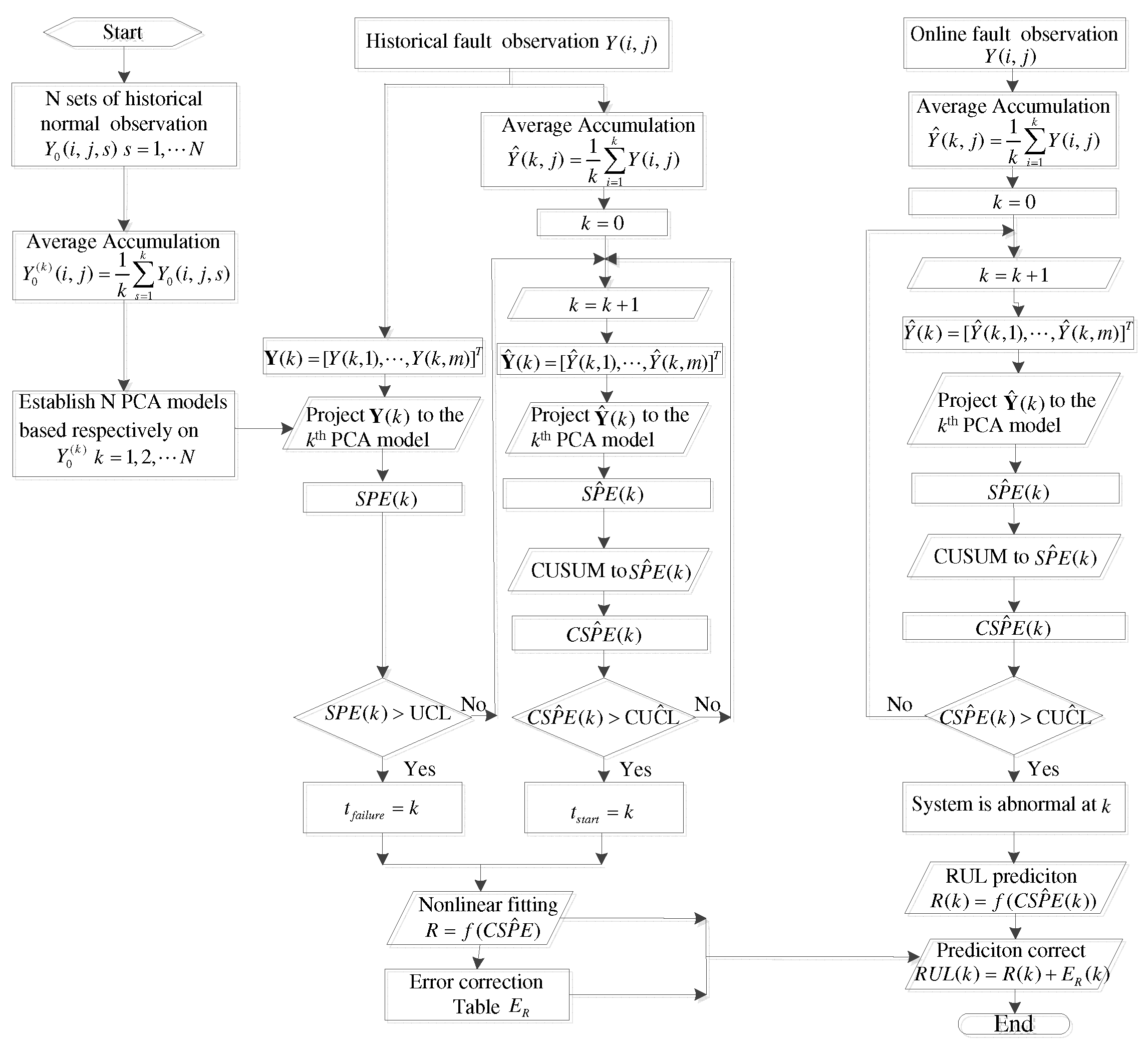
Figure 2.
Flowchart of CUSUM-AA-PCA based fault prognosis.

Figure 3.
SPE chart for PCA.

Figure 4.
SPE chart for CUSUM-PCA.

Figure 5.
SPE chart for WF-PCA.

Figure 6.
SPE chart for AA-PCA.

Figure 7.
SPE chart for CUSUM-AA-PCA.

Figure 8.
Shewhart chart of AA-DCA.

Figure 9.
Shewhart to , or for CUSUM-AA-DCA. The subfigures (a–c) are the Shewhart charts to , , or of CUSUM-AA-DCA. The subfigures (d–f) are the Shewhart charts to , , or of AA-DCA. The dotted red line is the control limit.
Figure 9.
Shewhart to , or for CUSUM-AA-DCA. The subfigures (a–c) are the Shewhart charts to , , or of CUSUM-AA-DCA. The subfigures (d–f) are the Shewhart charts to , , or of AA-DCA. The dotted red line is the control limit.

Figure 10.
SPE chart for PCA for historical fault observation.

Figure 11.
SPE chart for CUMSUM-AA-PCA to historical fault observation.

Figure 12.
The fitted RUL prediction model based on the SPE damage precursor.

Figure 13.
The error correction curve of SPE based prediction model.

Figure 14.
The fitted RUL prediction model based on DC corresponding to , and . The left part (a–c) is the fitted RUL prediction model for the three fault patterns corresponding to , , and , and the right part (d–f) is their model error correction curve.
Figure 14.
The fitted RUL prediction model based on DC corresponding to , and . The left part (a–c) is the fitted RUL prediction model for the three fault patterns corresponding to , , and , and the right part (d–f) is their model error correction curve.

Figure 15.
Online RUL prediction based on SPE.

Figure 16.
Online RUL prediction based on DC corresponding to , and .

Figure 17.
RUL prediction using AR to SPE.

Figure 18.
RUL prediction using AR to DC corresponding to , and .


Table 1.
Detection result of SPE chart for PCA.
| Method | Detection Point | FDR | MDR |
|---|---|---|---|
| PCA | 421 | 0% | 81.0412% |
| WF-PCA | 281 | 3.125% | 51.875% |
| CUMSUM-PCA | 311 | 0% | 58.125% |
| AA-PCA | 57 | 0% | 5.2083% |
| CUMSUM-AA-PCA | 44 | 0% | 2.5% |
Table 2.
Detection results of the Shewhart chart for DCA.
| Statistics | Method | Detection Point | FDR | MDR |
|---|---|---|---|---|
| DCA | 480 | 4.6875% | 75% | |
| CUMSUM-DCA | 419 | 0% | 27.3438% | |
| AA-DCA | 416 | 0% | 25% | |
| CUMSUM-AA-DCA | 403 | 0% | 14.8438% | |
| DCA | 470 | 0.7813% | 91.25 | |
| CUMSUM-DCA | 201 | 0% | 35.2083% | |
| AA-DCA | 60 | 0% | 5.8333% | |
| CUMSUM-AA-DCA | 52 | 0% | 4.1667% | |
| DCA | 512 | 0% | 99.6094 | |
| CUMSUM-DCA | 404 | 0% | 57.8125% | |
| AA-DCA | 305 | 0% | 19.1406% | |
| CUMSUM-AA-DCA | 278 | 0% | 8.5938% |
Table 3.
Mean of absolute RUL prediction error.
| Statistics | Exponential Fittting | Auto-Regressive |
|---|---|---|
| SPE | 2.0000 | 9.8084 |
| DC3 | 2.1846 | 2.5500 |
| DC5 | 6.5660 | 6.6320 |
| DC10 | 11.5484 | 19.6766 |
© 2018 by the authors. Licensee MDPI, Basel, Switzerland. This article is an open access article distributed under the terms and conditions of the Creative Commons Attribution (CC BY) license (http://creativecommons.org/licenses/by/4.0/).
Share and Cite
MDPI and ACS Style
Zhou, F.; Park, J.H.; Wen, C.; Hu, P. Average Accumulative Based Time Variant Model for Early Diagnosis and Prognosis of Slowly Varying Faults. Sensors 2018, 18, 1804. https://doi.org/10.3390/s18061804
AMA Style
Zhou F, Park JH, Wen C, Hu P. Average Accumulative Based Time Variant Model for Early Diagnosis and Prognosis of Slowly Varying Faults. Sensors. 2018; 18(6):1804. https://doi.org/10.3390/s18061804
Chicago/Turabian StyleZhou, Funa, Ju H. Park, Chenglin Wen, and Po Hu. 2018. "Average Accumulative Based Time Variant Model for Early Diagnosis and Prognosis of Slowly Varying Faults" Sensors 18, no. 6: 1804. https://doi.org/10.3390/s18061804
Note that from the first issue of 2016, this journal uses article numbers instead of page numbers. See further details here.