

An Autocollimator Axial Measurement Method Based on the Strapdown Inertial Navigation System
by
Wenjia Ma
1,2,
Jianrong Li
1,
Shaojin Liu
1,
Yan Han
1,2,
Xu Liu
1,2,
Zhiqian Wang
1,* and
Changhong Jiang
3,* 1
Changchun Institute of Optics, Fine Mechanics and Physics, Chinese Academy of Sciences, Changchun 130033, China
2
University of Chinese Academy of Sciences, Beijing 100049, China
3
School of Electrical and Electronic Engineering, Changchun University of Technology, Changchun 130012, China
*
Authors to whom correspondence should be addressed.
Sensors 2024, 24(8), 2590; https://doi.org/10.3390/s24082590
Submission received: 23 March 2024
/
Revised: 13 April 2024
/
Accepted: 16 April 2024
/
Published: 18 April 2024
(This article belongs to the Special Issue Photoelectric Measurement and Sensing: New Technology and Applications—2nd Edition)
Abstract
:Autocollimators are widely used optical axis-measuring tools, but their measurement errors increase significantly when measuring under non-leveled conditions and they have a limited measurement range due to the limitations of the measurement principle. To realize axis measurement under non-leveled conditions, this paper proposes an autocollimator axis measurement method based on the strapdown inertial navigation system (SINS). First, the measurement model of the system was established. This model applies the SINS to measure the change in attitude of the autocollimator. The autocollimator was then applied to measure the angular relationship between the measured axis and its own axis, based on which the angular relationship of the axis was measured via computation through signal processing and data fusion in a multi-sensor system. After analyzing the measurement errors of the system model, the Monte Carlo method was applied to carry out a simulation analysis. This showed that the majority of the measurement errors were within ±0.002° and the overall measurement accuracy was within ±0.006°. Tests using equipment with the same parameters as those used in the simulation analysis showed that the majority of the measurement errors were within ±0.004° and the overall error was within ±0.006°, which is consistent with the simulation results. This analysis proves that this method solves the problem of the autocollimator being unable to measure the axis under non-leveled conditions and meets the needs of axis measurement with the application of autocollimators under a moving base.
1. Introduction
Axis measurement is an essential method for determining relative position and attitude [1,2], and it is widely used in industrial production, military operations, aerospace, and other fields. It is also employed in scientific research, including in straightness calibration [3], photon energy detection [4], and surface measurement [5]. In the aspect of axis angle measurement, it can be divided into mechanical methods, electromagnetic methods, optical methods, and inertial methods [6]. Among them, the mechanical and electromagnetic methods are more mature and less expensive to measure. However, the accuracy of electrical methods is easily affected by the environment, while mechanical methods are mostly contact measurements, which are limited in many fields. Optical measurement is a non-contact measurement method with high accuracy and sensitivity, which is widely used.
As a type of optical axis-measuring equipment, autocollimators benefit from advantages such as a high measuring accuracy, wide range, and non-contact measurement. The working principle of autocollimator is to use the orientation of the reflected beam from the target for pose calculation, which can realize precise single- and multi-axis angle measurements.
As technology has developed, so have autocollimators, from the traditional optical autocollimators to photoelectric autocollimators. The latter replaces the human eye with sensors such as charge-coupled devices (CCDs), quadrant photodiodes (QPDs), position sensitive detectors (PSDs), or complementary metal oxide semiconductors (CMOSs) for measurement, which improves the resolution and measurement accuracy [7,8,9,10]. The current research on measurement methods based on autocollimators mainly includes several aspects such as improving the measurement accuracy, increasing the measurement range, and increasing the number of measurement targets. For example, the use of new sensors improves the measurement accuracy [11,12,13], the design of the optical system improves the measurement accuracy and range [3,14], and the design of cooperative targeting achieves the measurement of the target’s angle in three directions: yaw, pitch, and roll [15,16].
However, due to the limitation of the autocollimation measurement principle, its measurement range is mainly determined by the field of view of the optical system, the type of light source, and the image sensor, and usually the angular measurement range of the high-precision autocollimator is less than 1°, and the measurement distance is less than 50 m. In addition, in order to ensure measurement accuracy, the autocollimator needs to be roughly leveled with a geodetic coordinate system as a reference before use to avoid causing more significant measurement errors or making measurement impossible. However, in many measurement scenarios, it is impossible to level the autocollimator, which needs to remain stationary during the measurement process, making it impossible to carry out dynamic measurement. Therefore, autocollimators are usually used in the laboratory or after leveling on a stable platform. It is not possible to measure across long distances and on a large scale, such as, for example, in the case of ship installations, where the axes between the upper and lower layers of the hull are measured; in the case of large airplanes, where the axes are calibrated between each of the long-distance axes; or in the case of fast axes measurements of carrier vehicles in an off-site environment.
The principle of the strapdown inertial navigation system (SINS) is based on inertial characteristics; through the fusion data of the internal gyroscope and accelerometer sensors, it can realize accurate measurement of its angle and that of its strapdown equipment relative to the geodetic coordinate system. Accelerometers usually use micro-electromechanical system technology, and the displacement and angle can be inferred by integrating the acceleration in three directions [17,18,19]. Currently, the laser gyro and fiber-optic gyro measurement principles are based on the Sagnac effect, i.e., the beam propagation time slightly differs with rotation, and by measuring the time difference, the rotational speed and direction of an object can be obtained [20,21]. Compared with traditional gyroscopes, they have the advantages of high precision and shock resistance, so they are widely used in navigation systems [22,23].
At present, precision measurement is usually not limited to one kind of equipment, and multi-device cooperative work is one of the hot topics in current research [24,25]. With the improvement of the accuracy of laser gyro, fiber-optic gyro, and micro-electromechanical system (MEMS) inertial guidance technology, as well as the decrease in the cost and volume, inertial guidance has been employed in a large number of applications for the solution of position and navigation under multi-sensors. For example, inertial guidance is usually combined with a global navigation satellite system (GNSS) for integrated navigation [26,27,28], with a Doppler velocity log (DVL) for underwater navigation [29], and with a radar or camera for simultaneous localization and mapping (SLAM) algorithms [30].
Based on SINS characteristics and the defects that mean the autocollimator cannot measure under long-distance, wide-angle, or non-leveled conditions, it is of great practical significance and application value to proposes a non-leveled dynamic axis measurement method based on an SINS and autocollimator.
This paper is organized as follows: In Section 2, the system composition, measurement modeling, and experimental setups are described. Section 3 shows the simulation results and experimental results. Section 4 explains the experimental results, the potential limitations of this study, and how the system could be improved in future work. Section 5 presents the conclusions.
2. Methodologies
2.1. System Composition
Figure 1a shows the system composition, which includes a dual-axis photoelectric autocollimator and a strapdown inertial guide. The SINS consists of three fiber-optic gyros; it is a customized version purchased by the laboratory. The measurement errors of the inertial guide were within ±0.001° over a short time. The autocollimator consists of an optical system, a light source, and a CMOS sensor. The optical system was made by our lab and is designed for a focal length of 60 mm, an aperture of 25 mm, and a measuring range of 5 m. The model of the CMOS sensor is NOIP1SN5000A, made by ONSEMI, Scottsdale, AZ, USA; the sensor utilizes 4.8 μm × 4.8 μm pixels that support low-noise “pipelined” and “triggered” global shutter readout modes with 2592 × 2048 active pixels, with a plane mirror as the measurement target. The autocollimator has a measurement accuracy of ±0.001° in yaw and pitch under horizontal conditions, theoretically. The SINS has a measurement accuracy of ±0.01° theoretically, and had a measurement accuracy of ±0.001° in a short time proven by tests in the yaw, pitch, and roll directions. The measurement principle is shown in Figure 1b. In the measurement system, the inertial guide is used to measure the angular information between the system and O-XYZ relative to the geodetic coordinate system (i.e., northeast sky coordinate system), and the autocollimator is used to measure the angular relationship between the equipment and the YB axis of the target being measured (planar mirror). The fusion of the two data points is used to obtain the relationship between the axis of the target being measured relative to the geodetic coordinate system for the yaw and pitch angles.
2.2. Measurement Modeling
2.2.1. Coordinate System Establishment
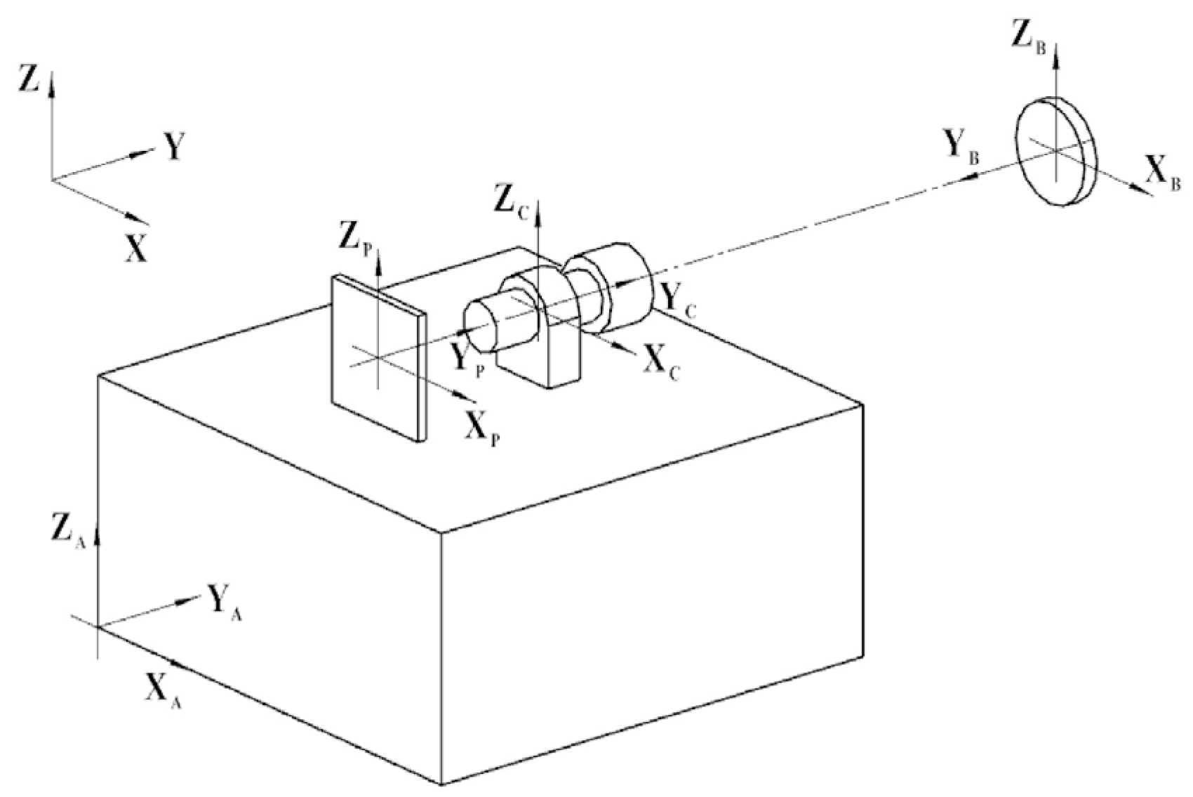
The first step in establishing the system measurement model is to establish the measurement coordinate system, as shown in Figure 2, with the plane mirror as the measurement target. O-XYZ is the geodetic coordinate system (i.e., the northeast celestial coordinate system), O-XAYAZA is the SINS coordinate system, O-XCYCZC is the lens coordinate system, O-XPYPZP is the camera coordinate system, and O-XBYBZB is the plane mirror coordinate system. Among them, the inertial coordinate system, the lens coordinate system, and the camera coordinate system are all based on the Earth’s level; the coordinate axes of these three coordinate systems are in the same direction, and the orientation is based on the YC direction along the optical axis.
2.2.2. Measurement Modeling of the Autocollimator
First, we consider the measurement model of the autocollimator in a leveled case. Projection along the opposite direction to the X-axis in Figure 2 yields the system shown in Figure 3. For this, we let the focal length of the autocollimator be f. The plane mirror reflects the emitted target, point P, to the image plane, point P (xp,zp). Then, the yaw angle α and pitch angle β of the plane mirror concerning the autocollimator can be computed using Equation (1).
A further analysis of the measurement system under non-leveled dynamic conditions is shown in Figure 4 for the O-XZ planar projection obtained by projecting the measurement coordinate system in Figure 2 along the positive direction of the Y-axis. When the roll angle between the autocollimator and the horizontal plane is γA, the target is set to image point P (xp,zp) on the image plane of the camera and converted from the O-XpZp coordinate system to the O-XZ coordinate system. The position coordinate conversion equations are as follows:
Substituting Equation (2) into (1) yields the relative value of the measurement target to the axis of the measurement system in the non-leveled state:
2.2.3. Measurement Modeling of the SINS
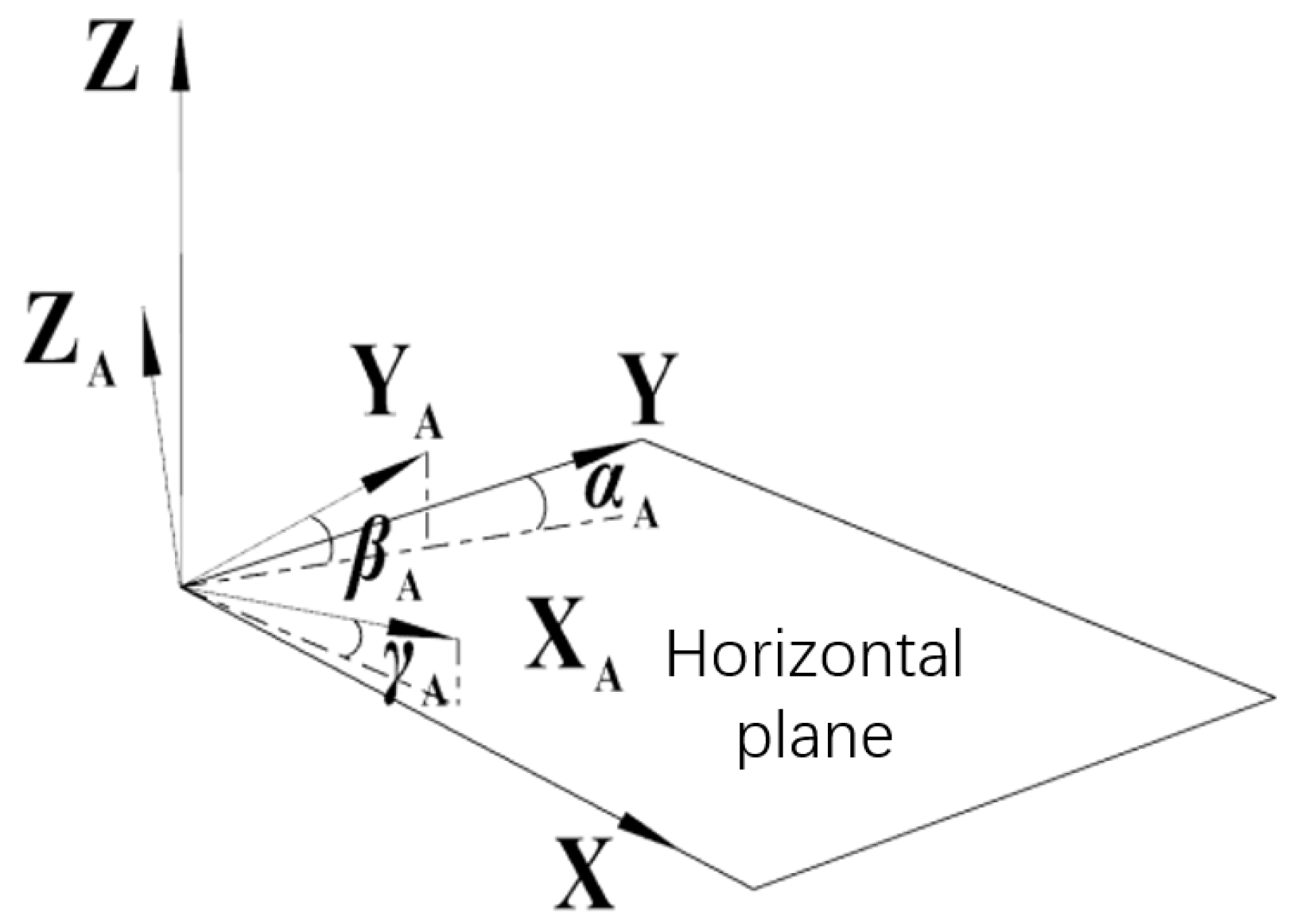
As shown in Figure 5, the inertial guidance measurement angles are defined, respectively, as follows:
- Yaw angle, αA: the horizontal angle between the projection of the YA-axis onto the horizontal plane and the actual north direction;
- Pitch angle, βA: the angle between the YA-axis in the vertical projection plane and the horizontal plane;
- Roll angle, γA: the angle between the XA-axis in the vertical projection plane and the horizontal plane.
Figure 5.
SINS measurement coordinate system. The yaw angle αA, pitch angle βA, and roll angle γA can be measured using the SINS.
Figure 5.
SINS measurement coordinate system. The yaw angle αA, pitch angle βA, and roll angle γA can be measured using the SINS.
Combined with Equation (3), the orientation and pitch angle of the measurement target relative to the geodetic coordinate system can be obtained as follows:
2.3. Measurement Error Analysis
Based on the measurement model and the calculation formulae provided in Section 2, the sources of errors in the measurement system are further analyzed to prove the validity of the measurement system and its measurement accuracy.
The measurement errors of the system include systematic errors and random errors. Using Equation (4), the systematic errors of the system include the installation errors and focal length errors, and the random errors include the pixel errors and SINS measurement errors.
2.3.1. Installation Errors
Due to the virtual axis of the SINS, it is difficult to achieve parallelism between the coordinate system of the SINS and the autocollimator’s coordinate system through installation and adjustment, which leads to a small deviation between the two coordinate systems. If we let the angle of the autocollimator rolling direction relative to the horizontal plane be γA, the angle between the autocollimator rolling axis and the inertial guide rolling axis be γ, and the angle between the inertial guide rolling axis and the horizontal plane be γ0, then we have
Substituting Equation (5) into (4), we obtain
From Equation (6), the roll angle γ between the SINS and the autocollimator affects the measurement results, and this error cannot be eliminated in the relative measurement.
This systematic error can usually be measured and corrected. The measurement of angle γ is usually realized through methods such as optical–mechanical calibration. However, the SINS cannot be measured accurately, because of its virtual axis. According to engineering experience, this measurement error can be controlled at about 10″, so the cross-roll error in the subsequent simulation is taken as γ = ±0.003°.
2.3.2. Focal Length Errors
The lens’s focal length is usually determined by the optical design, but manufacturing and mounting errors will cause the focal length to be inconsistent with the design value. According to engineering experience, the actual focal length of the lens can usually be controlled within 0.1–0.5% of the theoretical value. After calibration, the actual focal length value can be controlled within 0.1% [31]. In this study, the theoretical focal length of the self-collimator is 60 mm and the actual value after calibration measurement is 59.64 mm. Accordingly, the following simulation takes the focal length error value as ±0.05 mm.
2.3.3. Pixel Errors
In Equation (5), xp and zp are the coordinates of the target’s imaging position on the camera at the time of measurement. The errors in xp and zp are determined by the resolution of the camera image element. According to research on the pixel subdivision algorithm, the pixel errors can usually be reduced to within 0.1 pixels using differential calculation and other methods [32]. The actual camera pixel resolution used in this system is 4.8 μm. In order to ensure that the simulation was consistent with the actual test, the pixel error value was taken to be 0.5 pixels in the simulation process, which is 2.4 μm.
2.3.4. SINS Measurement Errors
From Section 2.2.2, the measurement error of the SINS is determined by its measurement accuracy. This system uses the fiber-optic inertial guide for measurement. For the measurement system in this study, the measurement is usually completed in a short period of time in a single power-up, so the effects of system errors can be ignored. The random errors of fiber-optic inertial guides include zero bias and noise. However, random errors usually have a negligible effect on the measurement results when measuring in a short period of time. After testing the inertial guide used in the system, it was proven that the measurement errors of this inertial guide were within ±0.001° over a short period of time, so this value was taken for the simulation.
2.4. Experiments
Experimental validation was carried out using laboratory equipment to verify the validity of the measurement model and simulation results. The instrumentation used in this testing included the SINS, an autocollimator, a roll adjustment stage, a plane mirror with a 2D adjustment stage, and a parallel light tube for measurements with the following accuracies:
- The installation error was taken as γ = ±0.003°;
- The focal length error was taken as ±0.05 mm;
- The CMOS sensor measurement error was taken as ±0.1 pixel;
- The SINS measurement error was taken as ±0.001° in yaw, pitch, and roll;
- The parallel light pipes had a measurement accuracy of ±0.2″ in yaw and pitch;
- The roll adjustment table had a ±15° adjustment range.
The experimental setup is shown in Figure 6. The experimental procedure was as follows: The measuring system (SINS with the autocollimator) was placed on the roll adjustment stage, and the plane mirror with the 2D adjustment stage was placed between the measuring system and the parallel light tube. Adjusting the 2D adjustment table changed the plane mirror’s axis, and its axis changes were monitored with the parallel light tube. Measurement started from the position when the SINS was horizontal, and the range of roll adjustment was ±10°, with an interval of 2° between each adjustment. After each set of the system’s roll values was adjusted, its yaw and pitch values were adjusted using the initial angle of the plane mirror as a reference. Each yaw and pitch adjustment interval was 0.2°, with a range of ±1°. The yaw and pitch values of each set of the plane mirror adjustments were recorded, as well as the coordinate points of the image obtained from the autocollimator in the image plane (xp,zp). A total of 121 sets of corresponding data values were obtained.
3. Results
3.1. Simulation Results
To ensure the accuracy and validity of the measurement model presented in Section 2.2, as well as the error analysis provided in Section 2.3, a Monte Carlo analysis based on Equation (6) was conducted. The Monte Carlo method, also known as the statistical test method, is a numerical simulation technique that focuses on probabilistic phenomena. Its fundamental principle is random sampling. By constructing a probabilistic model that closely represents the measurement system’s performance and running random trials, the simulation can replicate the system’s random measurement characteristics. The simulation results can be considered as actual measurement outcomes when the number of simulations is large enough. Substituting the four measurement error values from the error analysis in Section 2.3, all of the parameters used in the simulation were the same as those used in the experiments, specifically including the following:
- The installation error was taken as γ = ±0.003°;
- The focal length error was taken as ±0.05 mm;
- The CMOS sensor measurement error was taken as ±0.1 pixel;
- The SINS measurement error was taken as ±0.001° in yaw, pitch, and roll.
The specific calculation steps were as follows:
- Randomly generate an initial set of truth data, including the measurement of the system’s roll angle (within ±5°) and the yaw and pitch angles of the plane mirror axis measured with the autocollimator (within ±4.5°);
- Based on the generated truth data, back-project the theoretical truth data measured with the sensor, and randomly add the error data in Section 3.1 to them as the measurement data of the sensor;
- Substituting the sensor measurement data into Equation (4), recalculate the yaw and pitch angles of the plane mirror as measurements;
- Calculate the difference between the measured data and the true value data as the measurement error.
Scatter plots of the measurement errors of the system and the distribution of the errors when repeating the calculation 10,000 times are shown in Figure 7. The figures show that the system’s measurement errors are overwhelmingly within the range of ±0.002° and the overall measurement accuracy is within the range of ±0.006°. The mean square deviations of the yaw and pitch errors are σ_yaw = 0.0020° (1σ) and σ_pitch = 0.0019° (1σ).
3.2. Experimental Results
The data measured in Section 2.4 are listed in Table 1. The measurement group 0 includes the initial yaw and pitch values of the mirror, as well as the position of the reflected target. For measurement groups 1 to 5, we sequentially increased the yaw and pitch of the plane mirror by about 0.2° in the same direction, using measurement group 0 as a reference. For measurement groups 6 to 10, we sequentially increased the yaw and pitch of the plane mirror by about 0.2° in the other direction, using measurement group 0 as a reference. The exact amount of change was measured by means of a parallel light tube, and the corresponding xp and zp values were also recorded.
We substituted the xp and zp data in Table 1 into Equation (6) to calculate the measurement values of the mirror’s change in yaw and pitch. The measurement group 0 was also used as the initial value in these calculations, and the measured values were compared with the true values to obtain the errors. From these calculations, the measurement errors are shown in Table 2, and each measurement error matches those of the measurement groups in Table 1.
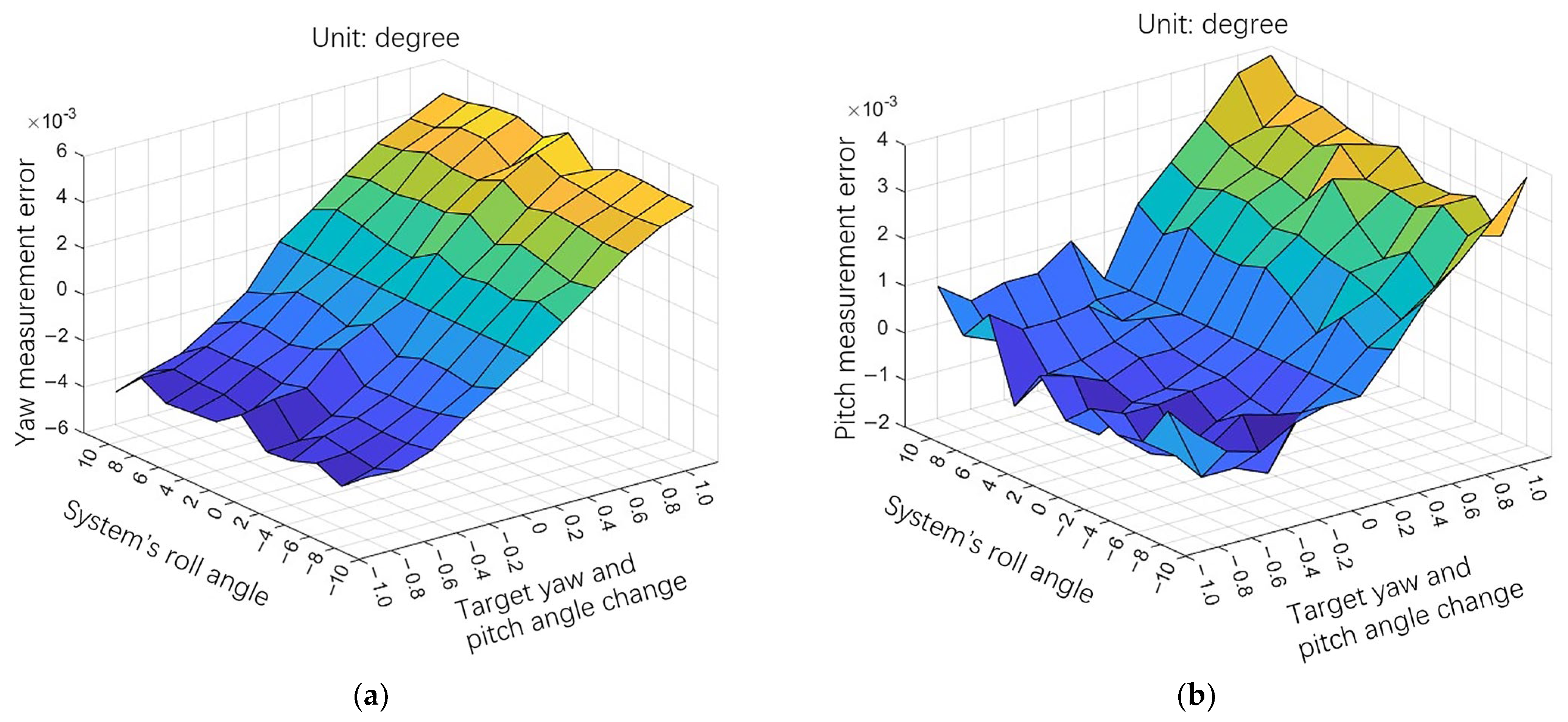
When the system measures within ±10° of the roll angle, most of the measurement errors are within ±0.004° and the overall error is within ±0.006°. The root mean square (RMS) values of the measurement errors are σ_yaw = 0.003° (1σ) and σ_pitch = 0.0018° (1σ). The measurement consistency is good, which is consistent with the simulation results.
4. Discussion
Through Monte Carlo simulation of this measurement model, the variance of the yaw and pitch is obtained as σ_yaw = 0.0020° (1σ) and σ_pitch = 0.0019° (1σ) after running the simulation 10,000 times. It can be deduced from the simulation results that the measurement error of this system is stable and consistent for the target yaw and pitch angles.
As can be seen from the experimental results, when the system roll angle is unchanged and the angle of the measurement target changes, the measurement error increases with the change in angle of the measurement target, and the sign of the measurement error is related to the sign of the change in angle of the target. Also, within a specific range, the system’s measurement error does not change due to the change in roll angle.
Comparing the experimental results with the simulation results, it can be seen that the yaw measurement error of the experimental results is larger than that of the simulation results. The reason for these different results may be the fact that the measurement group is too small to reflect the actual measurement capability of the system, or the fact that the CMOS sensor in the autocollimator does not coincide with the axis of the optical system when it is installed, or other reasons, which need to be further explored.
For axis measurements under non-leveled dynamic conditions, the accurate measurement of angles is usually achieved by optimizing the measurement environment, e.g., by designing vibration damping and leveling planes. This study started without optimizing the measurement equipment, which has an advantage in terms of preparation time, volume, and weight, although the accuracy is slightly lower in comparison. This measurement accuracy can still be suitable for vehicle-related axis measurement, aircraft axis measurement target calibration, and naval weapon axis measurement. Since the work presented in this paper involves only a measurement model and its validation under laboratory conditions, subsequent field tests need to be carried out to explore its engineering practicality further.
In this study, the data between the two sensors were only calculated and processed using the measurement model, but there may have been a time delay in the two sensors, which could have led to a decrease in the measurement accuracy due to the unsynchronized data when measuring on a dynamic platform; so, further exploration of data fusion and synchronization methods is required subsequently.
5. Conclusions
In order to realize axis measurement under non-leveled dynamic conditions using an autocollimator and extend the measuring range, an autocollimator axis measurement method based on the SINS is proposed. This article demonstrates the system model and measurement calculations, simulation analyses, and experimental verification of the model were carried out. The latter demonstrated that the majority of the method’s measurement errors were within ±0.002° and the overall measurement error was within ±0.006°. The measurement system was tested over a roll angle range of ±10°, showing that most of the measurement errors were within ±0.004° and the overall measurement error was within ±0.006°. This was consistent with the simulation results, showing a good measurement consistency.
Our system has certain advantages over other measurement methods, and the measurement accuracy can be further improved from the point of view of data fusion and synchronization of the two sensors in future work. According to the proposed study, a new measurement method can be provided for axis measurement in the case of a moving base.
Author Contributions
Conceptualization, W.M., C.J. and Z.W.; methodology, W.M., C.J. and Z.W.; software, S.L. and Z.W.; validation, W.M., Z.W. and J.L.; formal analysis, W.M. and Y.H.; investigation, Y.H.; resources, Z.W. and J.L.; data curation, W.M.; writing—original draft preparation, Z.W., X.L. and Y.H.; writing—review and editing, Z.W., Y.H., X.L., C.J. and J.L.; visualization, Z.W.; supervision, Z.W.; project administration, J.L. and Z.W.; funding acquisition, J.L. All authors have read and agreed to the published version of the manuscript.
Funding
This research was funded by the Scientific and Technological Development Program of Ji Lin Province, China (Grant No. 20210201048GX).
Institutional Review Board Statement
Not applicable.
Informed Consent Statement
Not applicable.
Data Availability Statement
The data presented in this study are available on request from the corresponding author.
Conflicts of Interest
The authors declare no conflicts of interest.
References
- Kumar, A.S.A.; George, B.; Mukhopadhyay, S.C. Technologies and Applications of Angle Sensors: A Review. IEEE Sens. J. 2021, 21, 7195–7206. [Google Scholar] [CrossRef]
- Gao, W.; Kim, S.W.; Bosse, H.; Haitjema, H.; Chena, Y.L.; Lu, X.D.; Knapp, W.; Weckenmann, A.; Estler, W.T.; Kunzmann, H. Measurement technologies for precision positioning. CIRP Ann.-Manuf. Technol. 2015, 64, 773–796. [Google Scholar] [CrossRef]
- Zheng, F.; Long, F.; Zhao, Y.; Yu, C.; Jia, P.; Zhang, B.; Yuan, D.; Feng, Q. High-Precision Small-Angle Measurement of Laser-Fiber Autocollimation Using Common-Path Polarized Light Difference. IEEE Sens. J. 2023, 23, 9237–9245. [Google Scholar] [CrossRef]
- Mandal, L.; Singh, J.; Ganesan, A.R. Michelson Interferometer with mirrored right-angled prism for measurement of tilt with double sensitivity. J. Opt. 2023, 53, 1545–1550. [Google Scholar] [CrossRef]
- Meng, F.; Yang, G.; Yang, J.; Lu, H.; Dong, Z.; Kang, R.; Guo, D.; Qin, Y. Error Analysis of Normal Surface Measurements Based on Multiple Laser Displacement Sensors. Sensors 2024, 24, 2059. [Google Scholar] [CrossRef] [PubMed]
- Wang, S.; Ma, R.; Cao, F.; Luo, L.; Li, X. A Review: High-Precision Angle Measurement Technologies. Sensors 2024, 24, 1755. [Google Scholar] [CrossRef] [PubMed]
- Zou, Y.; Zhang, N.; Yuan, H.; Liu, C.; Liu, D. High precision deflection angle measurement of irregular light spot. Chin. Space Sci. Technol. 2022, 42, 107–113. [Google Scholar]
- Guo, Y.; Cheng, H.; Liu, G. Three-degree-of-freedom autocollimation angle measurement method based on crosshair displacement and rotation. Rev. Sci. Instrum. 2023, 94, 0126806. [Google Scholar] [CrossRef] [PubMed]
- Yan, L.; Yan, Y.; Chen, B.; Lou, Y. A Differential Phase-Modulated Interferometer with Rotational Error Compensation for Precision Displacement Measurement. Appl. Sci. 2022, 12, 5002. [Google Scholar] [CrossRef]
- Kim, K.; Jang, K.W.; Ryu, J.K.; Jeong, K.H. Biologically inspired ultrathin arrayed camera for high-contrast and high-resolution imaging. Light Sci. Appl. 2020, 9, 28. [Google Scholar] [CrossRef]
- Guo, J.; Lin, L.; Li, S.; Chen, J.; Wang, S.; Wu, W.; Cai, J.; Zhou, T.; Liu, Y.; Huang, W. Ferroelectric superdomain controlled graphene plasmon for tunable mid-infrared photodetector with dual-band spectral selectivity. Carbon 2022, 189, 596–603. [Google Scholar] [CrossRef]
- Guo, J.; Lin, L.; Li, S.; Chen, J.; Wang, S.; Wu, W.; Cai, J.; Liu, Y.; Ye, J.; Huang, W. WSe2/MoS2 van der Waals Heterostructures Decorated with Au Nanoparticles for Broadband Plasmonic Photodetectors. ACS Appl. Nano Mater. 2022, 5, 587–596. [Google Scholar] [CrossRef]
- Guo, J.; Liu, Y.; Lin, L.; Li, S.; Cai, J.; Chen, J.; Huang, W.; Lin, Y.; Xu, J. Chromatic Plasmonic Polarizer-Based Synapse for All-Optical Convolutional Neural Network. Nano Lett. 2023, 23, 9651–9656. [Google Scholar] [CrossRef]
- Kong, Q.; Wen, L. Fast tilt measurement based on optical block. Opt. Laser Technol. 2022, 148, 107731. [Google Scholar] [CrossRef]
- Du, M.-x.; Yan, Y.-f.; Zhang, R.; Cai, C.-l.; Yu, X.; Bai, S.-p.; Yu, Y. 3D position angle measurement based on a lens array. Chin. Opt. 2022, 15, 45–55. [Google Scholar] [CrossRef]
- Ren, W.; Cui, J.; Tan, J. Precision roll angle measurement system based on autocollimation. Appl. Opt. 2022, 61, 3811–3818. [Google Scholar] [CrossRef] [PubMed]
- Dorofeev, N.V.; Kuzichkin, O.R.; Tsaplev, A.V. Accelerometric Method of Measuring the Angle of Rotation of the KinematicMechanisms of Nodes. Appl. Mech. Mater. 2015, 770, 592–597. [Google Scholar] [CrossRef]
- Gao, Y.; Zhang, X.; Mai, G.; Hu, R. Measurement Method for Angle Acceleration of Turn-table Based on Accelerometer. J. Astronaut. Metrol. Meas. 2015, 35, 14–16. [Google Scholar]
- Lu, Y.-l.; Pan, Y.-J.; Li, L.-l.; Liu, Y.; Peng, H. Measurement method of projectile’s heading and pitching angle velocities based on biaxial accelerometer. J. Chin. Inert. Technol. 2015, 23, 160–164. [Google Scholar]
- Ren, C.; Guo, D.; Zhang, L.; Wang, T. Research on Nonlinear Compensation of the MEMS Gyroscope under Tiny Angular Velocity. Sensors 2022, 22, 6577. [Google Scholar] [CrossRef]
- Lijia, Y.; Qiang, L.; Guochen, W.; Hualiang, S.; Qingzhi, Z. An on-orbit high-precision angular vibration measuring device based on laser gyro. Proc. SPIE 2022, 12169, 1216943. [Google Scholar]
- Liu, Y.; Luo, X.; Chen, X. Improvement of angle random walk of fiber-optic gyroscope using polarization-maintaining fiber ring resonator. Opt. Express 2022, 30, 29900–29906. [Google Scholar] [CrossRef] [PubMed]
- Ma, R.; Yu, H.; Ni, K.; Zhou, Q.; Li, X.; Wu, G. Angular velocity measurement system based on optical frequency comb. In Proceedings of the Conference on Semiconductor Lasers and Applications IX, Hangzhou, China, 21–23 October 2019. [Google Scholar]
- Ren, Y.; Zhang, F.; Liu, F.; Hu, X.; Fu, Y. Accuracy test method of multi-instrument cooperative measurement. Proc. SPIE 2022, 12282, 1228219. [Google Scholar]
- Kim, J.-A.; Lee, J.Y.; Kang, C.-S.; Woo, J.H. Hybrid optical measurement system for evaluation of precision two-dimensional planar stages. Measurement 2022, 194, 111023. [Google Scholar] [CrossRef]
- Suvorkin, V.; Garcia-Fernandez, M.; González-Casado, G.; Li, M.; Rovira-Garcia, A. Assessment of Noise of MEMS IMU Sensors of Different Grades for GNSS/IMU Navigation. Sensors 2024, 24, 1953. [Google Scholar] [CrossRef] [PubMed]
- Chang, L.; Bian, Q.; Zuo, Y.; Zhou, Q. SINS/GNSS-Integrated Navigation Based on Group Affine SINS Mechanization in Local-Level Frame. IEEE/ASME Trans. Mechatron. 2023, 28, 2471–2482. [Google Scholar] [CrossRef]
- Zhao, L.; Kang, Y.; Cheng, J.; Fan, R. A MFKF Based SINS/DVL/USBL Integrated Navigation Algorithm for Unmanned Underwater Vehicles in Polar Regions. In Proceedings of the 2019 Chinese Control Conference (CCC), Guangzhou, China, 27–30 July 2019; pp. 3875–3880. [Google Scholar] [CrossRef]
- Liu, X.; Liu, X.; Wang, L.; Huang, Y.; Wang, Z. SINS/DVL Integrated System with Current and Misalignment Estimation for Midwater Navigation. IEEE Access 2021, 9, 51332–51342. [Google Scholar] [CrossRef]
- Feng, L.; Qu, X.; Ye, X.; Wang, K.; Li, X. Fast Feature Matching in Visual-Inertial SLAM. In Proceedings of the 2022 17th International Conference on Control, Automation, Robotics and Vision (ICARCV), Singapore, 11–13 December 2022; pp. 500–504. [Google Scholar] [CrossRef]
- Cheng, Q.; Hu, H.; Li, L.; Wang, X.; Luo, X.; Zhang, X. Distortion analysis and focal length testing of off-axis optical system. Opt. Precis. Eng. 2022, 30, 2839–2846. [Google Scholar] [CrossRef]
- Wei, M.S.; Xing, F.; You, Z. A real-time detection and positioning method for small and weak targets using a 1D morphology-based approach in 2D images. Light Sci. Appl. 2018, 3, 18006. [Google Scholar] [CrossRef]
Figure 1.
System composition and principle. (a) The system includes an autocollimator and a strapdown inertial guide as the measurement equipment and a plane mirror as the target; (b) the autocollimator measures the plane mirror’s axis and the SINS measures the geodetic coordinate system. The red arrows represent the return of beam from the collimator after reflection by the plane mirror.

Figure 2.
Measurement coordinate system. The measurement model is constructed using the geodetic coordinate system O-XYZ, the SINS coordinate system O-XAYAZA, the lens coordinate system O-XCYCZC, the camera coordinate system O-XPYPZP, and the plane mirror coordinate system O-XBYBZB.
Figure 2.
Measurement coordinate system. The measurement model is constructed using the geodetic coordinate system O-XYZ, the SINS coordinate system O-XAYAZA, the lens coordinate system O-XCYCZC, the camera coordinate system O-XPYPZP, and the plane mirror coordinate system O-XBYBZB.

Figure 3.
Autocollimator measurement coordinate system. By calculating the position of the reflected point P (xp,zp), the yaw angle α and pitch angle β of the plane mirror concerning the autocollimator can be obtained.
Figure 3.
Autocollimator measurement coordinate system. By calculating the position of the reflected point P (xp,zp), the yaw angle α and pitch angle β of the plane mirror concerning the autocollimator can be obtained.
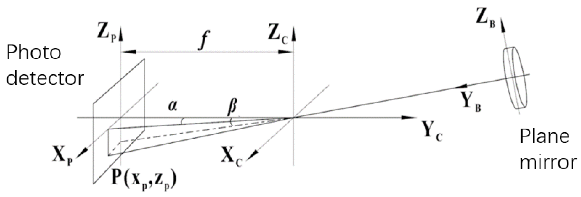
Figure 4.
Autocollimator angle measurement under non-leveled conditions. γA is the roll angle between the autocollimator and the horizontal plane, which causes measurement errors.
Figure 4.
Autocollimator angle measurement under non-leveled conditions. γA is the roll angle between the autocollimator and the horizontal plane, which causes measurement errors.

Figure 6.
Experimental setup, including a measurement system, a plane mirror (measurement target), and a parallel optical tube to measure the true value of the amount of change in the target. The measurement accuracy of the system is verified by changing the angle of the plane mirror.
Figure 6.
Experimental setup, including a measurement system, a plane mirror (measurement target), and a parallel optical tube to measure the true value of the amount of change in the target. The measurement accuracy of the system is verified by changing the angle of the plane mirror.
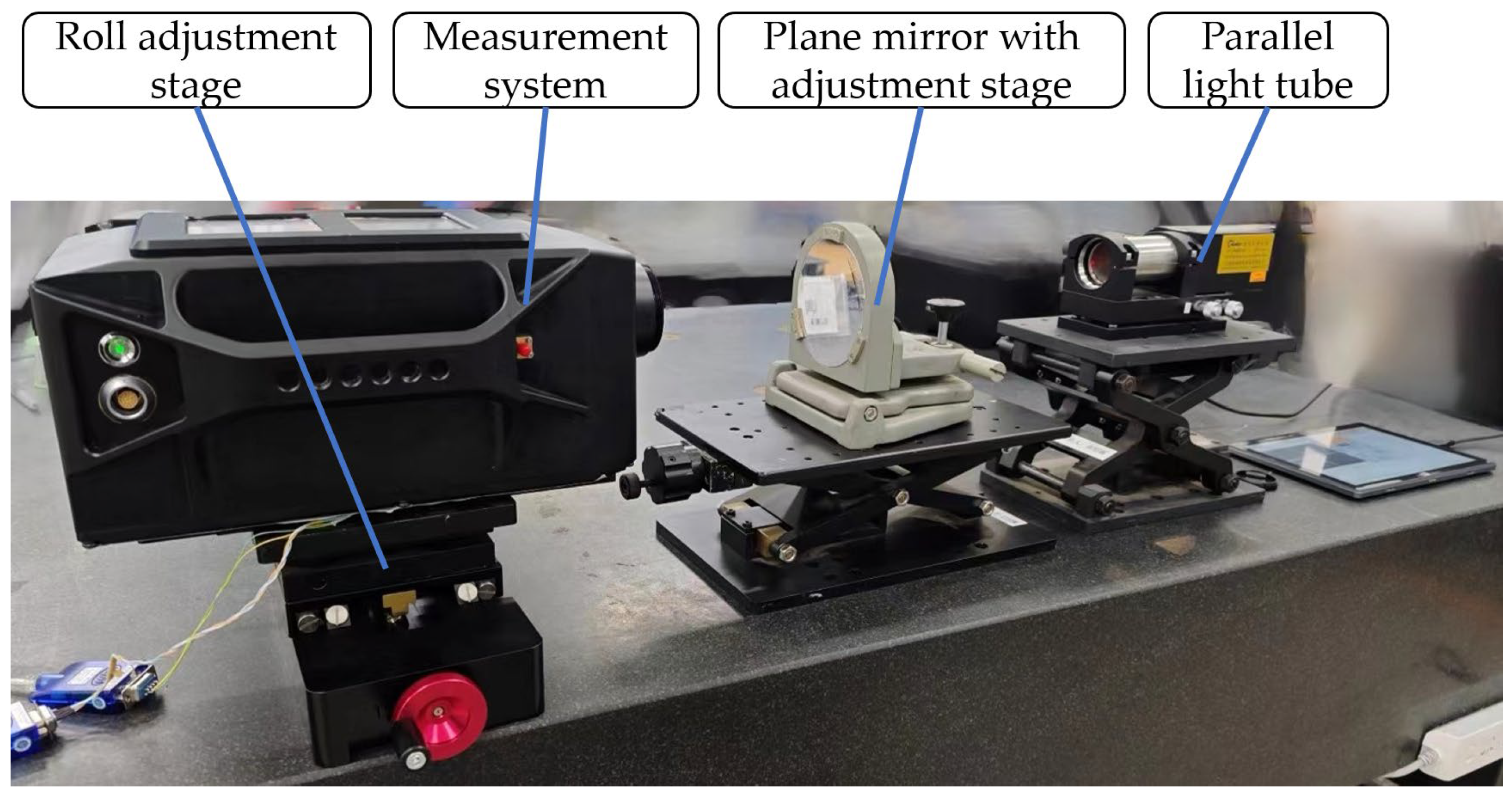
Figure 7.
Simulation results. The red line refers to the probability distribution curve fitted to the simulated data. (a) Yaw error scatter plot; (b) pitch error scatter plot; (c) yaw error histogram; (d) pitch error histogram.
Figure 7.
Simulation results. The red line refers to the probability distribution curve fitted to the simulated data. (a) Yaw error scatter plot; (b) pitch error scatter plot; (c) yaw error histogram; (d) pitch error histogram.

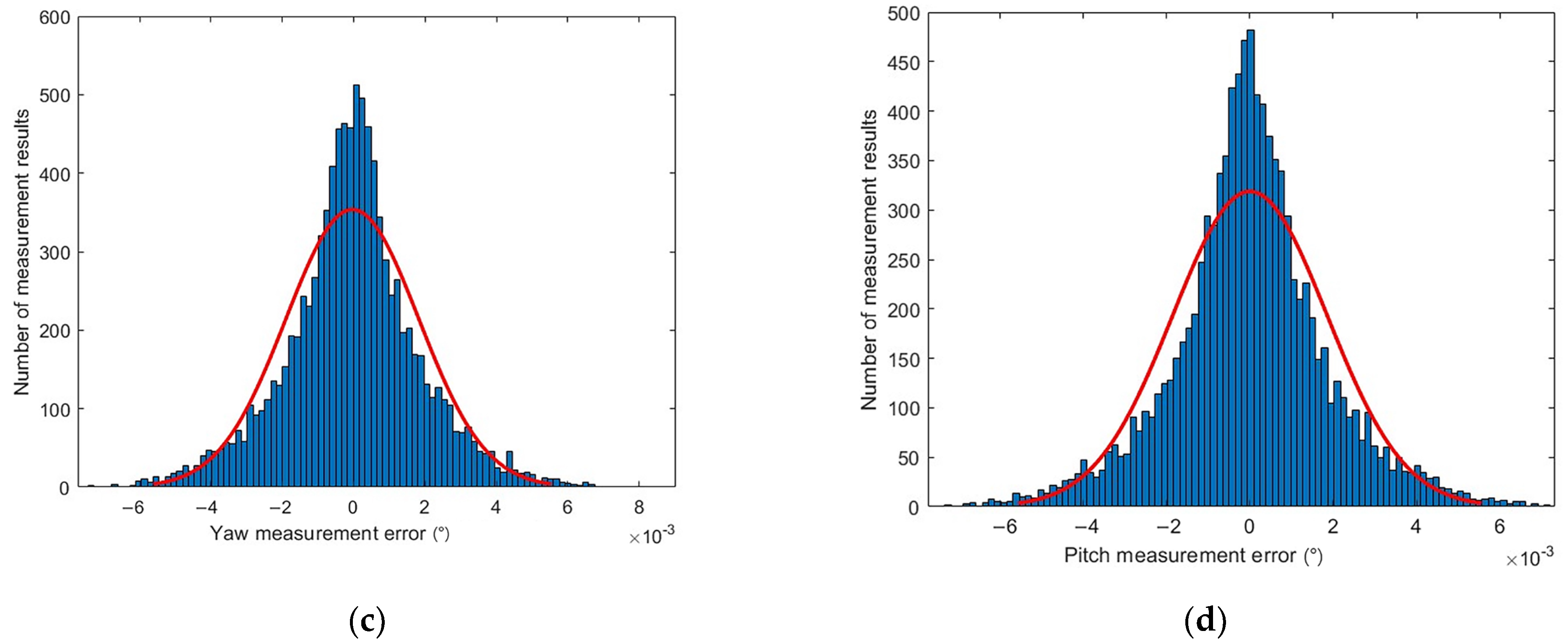
Figure 8.
Experimental error distribution. Different color represents the amount of the surface in the z-axis direction. (a) Yaw error distribution; (b) pitch error distribution.
Figure 8.
Experimental error distribution. Different color represents the amount of the surface in the z-axis direction. (a) Yaw error distribution; (b) pitch error distribution.


Table 1.
Experimental data.
| Roll Angle (°) | Data Type | Measurement Groups | ||||||||||
|---|---|---|---|---|---|---|---|---|---|---|---|---|
| 0 | 1 | 2 | 3 | 4 | 5 | 6 | 7 | 8 | 9 | 10 | ||
| −0.001 | Mirror yaw (°) | 58.9891 | 59.1843 | 59.3862 | 59.5881 | 59.7882 | 59.9858 | 58.7882 | 58.5838 | 58.3834 | 58.1838 | 57.9819 |
| Mirror pitch (°) | 90.2941 | 90.4921 | 90.6908 | 90.8952 | 91.0932 | 91.2998 | 90.0947 | 89.8982 | 89.6941 | 89.4959 | 89.2971 | |
| xp in CMOS | 996.21 | 1082.25 | 1171.07 | 1259.81 | 1347.67 | 1434.39 | 908.08 | 818.45 | 730.23 | 642.92 | 554.45 | |
| zp in CMOS | 985.64 | 1072.45 | 1159.24 | 1248.72 | 1334.92 | 1425.21 | 898.62 | 812.91 | 723.92 | 637.33 | 550.85 | |
| 2.010 | Mirror yaw (°) | 58.9342 | 59.1346 | 59.3338 | 59.5343 | 59.7375 | 59.9371 | 58.7369 | 58.5367 | 58.3347 | 58.1356 | 57.9309 |
| Mirror pitch (°) | 90.2945 | 90.4973 | 90.6951 | 90.8961 | 91.0947 | 91.2951 | 90.0933 | 89.8943 | 89.6949 | 89.4949 | 89.2946 | |
| xp in CMOS | 996.78 | 1081.68 | 1166.11 | 1251.16 | 1337.37 | 1421.56 | 912.98 | 828.17 | 742.57 | 658.29 | 571.78 | |
| zp in CMOS | 985.57 | 1077.33 | 1166.81 | 1257.67 | 1347.51 | 1437.87 | 894.77 | 805.01 | 715.01 | 624.82 | 534.54 | |
| 4.002 | Mirror yaw (°) | 58.9664 | 59.1654 | 59.3642 | 59.5692 | 59.7686 | 59.9669 | 58.7627 | 58.5658 | 58.3646 | 58.1605 | 57.9634 |
| Mirror pitch (°) | 90.2976 | 90.4936 | 90.6922 | 90.8951 | 91.0959 | 91.2957 | 90.0921 | 89.8914 | 89.6961 | 89.4982 | 89.2925 | |
| xp in CMOS | 996.29 | 1077.64 | 1158.83 | 1242.53 | 1323.64 | 1404.31 | 913.21 | 832.94 | 750.86 | 667.69 | 587.58 | |
| zp in CMOS | 985.66 | 1077.11 | 1170.01 | 1264.51 | 1358.31 | 1451.31 | 889.87 | 796.47 | 705.27 | 613.01 | 517.77 | |
| 6.003 | Mirror yaw (°) | 58.9835 | 59.1883 | 59.3879 | 59.5843 | 59.7841 | 59.9892 | 58.7867 | 58.5819 | 58.3824 | 58.1865 | 57.9832 |
| Mirror pitch (°) | 90.2931 | 90.4925 | 90.6961 | 90.8969 | 91.0935 | 91.2999 | 90.0967 | 89.8933 | 89.6947 | 89.4956 | 89.2954 | |
| xp in CMOS | 996.43 | 1076.82 | 1154.83 | 1231.56 | 1309.67 | 1389.84 | 919.34 | 839.02 | 761.07 | 684.71 | 605.31 | |
| zp in CMOS | 985.58 | 1081.81 | 1179.34 | 1275.66 | 1370.41 | 1469.31 | 891.17 | 793.71 | 698.31 | 603.02 | 507.11 | |
| 8.007 | Mirror yaw (°) | 59.0043 | 59.2053 | 59.4065 | 59.6031 | 59.8038 | 60.0064 | 58.8056 | 58.6067 | 58.4061 | 58.2053 | 58.0048 |
| Mirror pitch (°) | 90.2923 | 90.4947 | 90.6924 | 90.8946 | 91.0965 | 91.2957 | 90.0921 | 89.8955 | 89.6918 | 89.4951 | 89.2913 | |
| xp in CMOS | 996.53 | 1071.88 | 1147.14 | 1220.53 | 1295.46 | 1371.41 | 922.08 | 847.62 | 772.76 | 697.43 | 622.66 | |
| zp in CMOS | 985.35 | 1085.26 | 1182.96 | 1282.49 | 1382.28 | 1480.58 | 886.62 | 789.21 | 689.19 | 592.02 | 492.45 | |
| 10.005 | Mirror yaw (°) | 59.0086 | 59.2059 | 59.4079 | 59.6074 | 59.8075 | 60.0061 | 58.8081 | 58.6015 | 58.4021 | 58.2022 | 58.0018 |
| Mirror pitch (°) | 90.2878 | 90.4854 | 90.6857 | 90.8844 | 91.0879 | 91.2847 | 90.0821 | 89.8816 | 89.6849 | 89.4802 | 89.2815 | |
| xp in CMOS | 996.58 | 1066.86 | 1139.08 | 1210.33 | 1281.35 | 1352.29 | 924.97 | 850.85 | 779.46 | 708.71 | 637.19 | |
| zp in CMOS | 985.35 | 1085.76 | 1187.43 | 1288.21 | 1391.17 | 1490.91 | 882.17 | 780.19 | 680.59 | 577.41 | 477.05 | |
| −2.006 | Mirror yaw (°) | 58.9537 | 59.1531 | 59.3571 | 59.5554 | 59.7552 | 59.9555 | 58.7547 | 58.5509 | 58.3521 | 58.1568 | 57.9529 |
| Mirror pitch (°) | 90.2958 | 90.4984 | 90.6992 | 90.8985 | 91.0972 | 91.2952 | 90.0911 | 89.8948 | 89.6965 | 89.4907 | 89.2906 | |
| xp in CMOS | 996.41 | 1087.01 | 1179.91 | 1270.05 | 1360.52 | 1451.51 | 905.81 | 813.51 | 723.12 | 634.23 | 542.01 | |
| zp in CMOS | 985.56 | 1071.19 | 1155.72 | 1239.63 | 1323.51 | 1406.63 | 899.65 | 817.05 | 733.63 | 647.11 | 563.26 | |
| −4.004 | Mirror yaw (°) | 59.0021 | 59.2047 | 59.4041 | 59.6004 | 59.8015 | 60.0088 | 58.8028 | 58.6031 | 58.4021 | 58.2037 | 58.0012 |
| Mirror pitch (°) | 90.2947 | 90.4979 | 90.6974 | 90.8953 | 91.0954 | 91.2957 | 90.0922 | 89.8922 | 89.6928 | 89.4938 | 89.2909 | |
| xp in CMOS | 996.21 | 1091.18 | 1184.89 | 1276.97 | 1371.23 | 1468.07 | 902.77 | 809.02 | 715.01 | 622.04 | 527.32 | |
| zp in CMOS | 985.37 | 1067.94 | 1148.86 | 1229.01 | 1310.05 | 1390.91 | 903.54 | 822.61 | 742.01 | 661.53 | 579.94 | |
| −6.000 | Mirror yaw (°) | 58.9945 | 59.1977 | 59.3999 | 59.5983 | 59.7976 | 59.9975 | 58.7913 | 58.5925 | 58.3916 | 58.1939 | 57.9945 |
| Mirror pitch (°) | 90.2922 | 90.4963 | 90.6957 | 90.8931 | 91.0932 | 91.2976 | 90.0955 | 89.8923 | 89.6914 | 89.4948 | 89.2926 | |
| xp in CMOS | 996.27 | 1094.52 | 1191.97 | 1287.85 | 1383.99 | 1480.52 | 898.61 | 802.44 | 705.53 | 610.31 | 514.13 | |
| zp in CMOS | 985.32 | 1064.99 | 1142.36 | 1218.89 | 1296.79 | 1376.34 | 909.37 | 830.68 | 752.81 | 676.65 | 598.34 | |
| −8.001 | Mirror yaw (°) | 58.9714 | 59.1781 | 59.3785 | 59.5754 | 59.7751 | 59.9758 | 58.7727 | 58.5719 | 58.3701 | 58.1722 | 57.9702 |
| Mirror pitch (°) | 90.2911 | 90.4971 | 90.6935 | 90.8979 | 91.0926 | 91.2933 | 90.0906 | 89.8917 | 89.6966 | 89.4977 | 89.2969 | |
| xp in CMOS | 996.14 | 1098.83 | 1197.91 | 1296.01 | 1394.55 | 1494.01 | 897.39 | 798.02 | 698.53 | 600.47 | 500.78 | |
| zp in CMOS | 985.68 | 1062.31 | 1135.11 | 1211.58 | 1283.52 | 1358.11 | 911.36 | 837.71 | 765.87 | 692.09 | 617.83 | |
| −10.006 | Mirror yaw (°) | 58.9665 | 59.1671 | 59.3617 | 59.5681 | 59.7611 | 59.9665 | 58.7616 | 58.5667 | 58.3666 | 58.1639 | 57.9635 |
| Mirror pitch (°) | 90.2917 | 90.4933 | 90.6942 | 90.8944 | 91.0939 | 91.2957 | 90.0971 | 89.8946 | 89.6902 | 89.4913 | 89.2969 | |
| xp in CMOS | 996.36 | 1098.48 | 1198.05 | 1302.56 | 1401.21 | 1505.27 | 893.01 | 793.38 | 691.28 | 588.71 | 487.71 | |
| zp in CMOS | 985.79 | 1057.29 | 1129.02 | 1199.38 | 1270.61 | 1341.91 | 917.94 | 845.85 | 773.25 | 703.45 | 635.44 | |
Table 2.
Measurement errors.
| Roll Angle (°) | Data Type | Measurement Groups | |||||||||
|---|---|---|---|---|---|---|---|---|---|---|---|
| 1 | 2 | 3 | 4 | 5 | 6 | 7 | 8 | 9 | 10 | ||
| −0.001 | Yaw error (°) | 0.0016 | 0.0029 | 0.0040 | 0.0048 | 0.0053 | −0.0007 | −0.0014 | −0.0027 | −0.0028 | −0.0031 |
| Pitch error (°) | 0.0013 | 0.0018 | 0.0028 | 0.0026 | 0.0031 | −0.0004 | −0.0007 | −0.0008 | −0.0013 | −0.0008 | |
| 2.010 | Yaw error (°) | 0.0011 | 0.0021 | 0.0033 | 0.0043 | 0.0042 | −0.0016 | −0.0025 | −0.0034 | −0.0041 | −0.0042 |
| Pitch error (°) | 0.0009 | 0.0016 | 0.0021 | 0.0026 | 0.0026 | −0.0004 | −0.0005 | −0.0006 | −0.0006 | −0.0003 | |
| 4.002 | Yaw error (°) | 0.0013 | 0.0026 | 0.0036 | 0.0042 | 0.0047 | −0.0012 | −0.0024 | −0.0030 | −0.0034 | −0.0041 |
| Pitch error (°) | 0.0004 | 0.0015 | 0.0016 | 0.0025 | 0.0026 | −0.0006 | −0.0009 | −0.0013 | −0.0012 | −0.0006 | |
| 6.003 | Yaw error (°) | 0.0011 | 0.0023 | 0.0035 | 0.0040 | 0.0047 | −0.0012 | −0.0024 | −0.0031 | −0.0036 | −0.0037 |
| Pitch error (°) | 0.0010 | 0.0013 | 0.0020 | 0.0028 | 0.0028 | −0.0007 | −0.0005 | −0.0010 | −0.0010 | −0.0005 | |
| 8.007 | Yaw error (°) | 0.0015 | 0.0020 | 0.0033 | 0.0040 | 0.0046 | −0.0014 | −0.0022 | −0.0031 | −0.0038 | −0.0042 |
| Pitch error (°) | 0.0006 | 0.0010 | 0.0015 | 0.0024 | 0.0022 | −0.0004 | −0.0015 | −0.0012 | −0.0012 | 0.0004 | |
| 10.005 | Yaw error (°) | 0.0011 | 0.0022 | 0.0033 | 0.0041 | 0.0046 | −0.0010 | −0.0019 | −0.0029 | −0.0034 | −0.0033 |
| Pitch error (°) | 0.0008 | 0.0017 | 0.0023 | 0.0030 | 0.0037 | 0 | −0.0002 | −0.0006 | −0.0004 | 0.0002 | |
| −2.006 | Yaw error (°) | 0.0009 | 0.0025 | 0.0035 | 0.0037 | 0.0046 | −0.0013 | −0.0019 | −0.0030 | −0.0039 | −0.0039 |
| Pitch error (°) | 0.0011 | 0.0017 | 0.0021 | 0.0031 | 0.0029 | −0.0003 | −0.0003 | −0.0006 | −0.0003 | −0.0001 | |
| −4.004 | Yaw error (°) | 0.0010 | 0.0025 | 0.0035 | 0.0044 | 0.0050 | −0.0009 | −0.0022 | −0.0028 | −0.0036 | −0.0040 |
| Pitch error (°) | 0.0011 | 0.0020 | 0.0023 | 0.0028 | 0.0030 | 0.0001 | −0.0002 | −0.0004 | −0.0005 | −0.0010 | |
| −6.000 | Yaw error (°) | 0.0013 | 0.0023 | 0.0037 | 0.0044 | 0.0049 | −0.0008 | −0.0020 | −0.0029 | −0.0036 | −0.0041 |
| Pitch error (°) | 0.0014 | 0.0020 | 0.0023 | 0.0030 | 0.0032 | −0.0002 | 0.0003 | 0.0002 | 0.0002 | 0.0007 | |
| −8.001 | Yaw error (°) | 0.0015 | 0.0024 | 0.0033 | 0.0039 | 0.0046 | −0.0014 | −0.0022 | −0.0029 | −0.0035 | −0.0035 |
| Pitch error (°) | 0.0010 | 0.0018 | 0.0025 | 0.0027 | 0.0032 | 0 | −0.0003 | −0.0003 | −0.0003 | −0.0005 | |
| −10.006 | Yaw error (°) | 0.0010 | 0.0021 | 0.0031 | 0.0038 | 0.0045 | −0.0018 | −0.0028 | −0.0037 | −0.0041 | −0.0046 |
| Pitch error (°) | 0.0014 | 0.0021 | 0.0028 | 0.0036 | 0.0038 | 0.0010 | −0.0005 | 0.0005 | 0.0003 | 0.0008 | |
Disclaimer/Publisher’s Note: The statements, opinions and data contained in all publications are solely those of the individual author(s) and contributor(s) and not of MDPI and/or the editor(s). MDPI and/or the editor(s) disclaim responsibility for any injury to people or property resulting from any ideas, methods, instructions or products referred to in the content. |
© 2024 by the authors. Licensee MDPI, Basel, Switzerland. This article is an open access article distributed under the terms and conditions of the Creative Commons Attribution (CC BY) license (https://creativecommons.org/licenses/by/4.0/).
Share and Cite
MDPI and ACS Style
Ma, W.; Li, J.; Liu, S.; Han, Y.; Liu, X.; Wang, Z.; Jiang, C. An Autocollimator Axial Measurement Method Based on the Strapdown Inertial Navigation System. Sensors 2024, 24, 2590. https://doi.org/10.3390/s24082590
AMA Style
Ma W, Li J, Liu S, Han Y, Liu X, Wang Z, Jiang C. An Autocollimator Axial Measurement Method Based on the Strapdown Inertial Navigation System. Sensors. 2024; 24(8):2590. https://doi.org/10.3390/s24082590
Chicago/Turabian StyleMa, Wenjia, Jianrong Li, Shaojin Liu, Yan Han, Xu Liu, Zhiqian Wang, and Changhong Jiang. 2024. "An Autocollimator Axial Measurement Method Based on the Strapdown Inertial Navigation System" Sensors 24, no. 8: 2590. https://doi.org/10.3390/s24082590
Note that from the first issue of 2016, this journal uses article numbers instead of page numbers. See further details here.