Time Series Forecasting Energy-efficient Organization of Wireless Sensor Networks

State Key Laboratory of Precision Measurement Technology and Instruments, Department of Precision Instruments, Tsinghua University, Beijing 100084, P. R. China
*
Author to whom correspondence should be addressed.
Sensors 2007, 7(9), 1766-1792; https://doi.org/10.3390/s7091766
Submission received: 9 August 2007
/
Accepted: 4 September 2007
/
Published: 5 September 2007
(This article belongs to the Special Issue Energy Efficiency and Intelligent Signal Processing for Wireless Sensing)
Abstract
:Due to their wide potential applications, wireless sensor networks have recently received tremendous attention. The strict energy constraints of sensor nodes result in the great challenges for energy efficiency. This paper investigates the energy efficiency problem and proposes an energy-efficient organization method with time series forecasting. The organization of wireless sensor networks is formulated for target tracking. Target model, multi-sensor model and energy model are defined accordingly. For the target tracking application, target localization is achieved by collaborative sensing with multi-sensor fusion. The historical localization results are utilized for adaptive target trajectory forecasting. Empirical mode decomposition is implemented to extract the inherent variation modes in the time series of a target trajectory. Future target position is derived from autoregressive moving average (ARMA) models, which forecast the decomposition components, respectively. Moreover, the energy-efficient organization method is presented to enhance the energy efficiency of wireless sensor networks. The sensor nodes implement sensing tasks according to the probability awakening in a distributed manner. When the sensor nodes transfer their observations to achieve data fusion, the routing scheme is obtained by ant colony optimization. Thus, both the operation and communication energy consumption can be minimized. Experimental results verify that the combination of the ARMA model and empirical mode decomposition can estimate the target position efficiently and energy saving is achieved by the proposed organization method in wireless sensor networks.
1. Introduction
Ubiquitous computing is emerging as a potential solution for wide sensing applications in the physical world. Thus, wireless sensor networks (WSNs) have become a growing research field. In WSNs, a large number of intelligent sensor nodes are integrated into the environment to accomplish complicated sensing tasks. Sensing, processing and communication capabilities are enabled on each sensor node. As sensor nodes usually work in unsupervised areas, the batteries cannot be easily recharged or replaced. Due to the limited battery life, the energy efficiency of a WSN is an important issue. Sleeping and awakening of sensor nodes are supported in power-aware hardware design [1]. By adopting proper energy management methods, the energy consumption of WSNs is scalable [2,3]. However, WSN is application-oriented and so is its energy consumption. As a typical application of WSN, target tracking should be addressed in the energy efficiency problem. In target tracking applications, energy-aware methods will be geared specially towards the target motion information. The prior target position estimation can be used to organize the awakening and routing of WSN so that the energy efficiency can be improved. Traditional target tracking is usually performed by a Kalman filter (KF) [4]. However, it is extremely challenging to implement a KF to track a maneuvering target if the dynamic model of target is highly nonlinear. Although a standard particle filter (PF) [5] can solve nonlinear non-Gaussian problems, it can not solve the estimation error cumulating problems when maneuvering occurs. Furthermore, although some algorithms have been proposed for maneuvering target tracking, such as the unscented particle filter (UPF) [6], these algorithms are computationally-expensive for sensor nodes. Hence, adaptive estimation can be provided by autoregressive moving average (ARMA) models. Forecasting with ARMA models has been utilized in many scenarios as they are capable of modeling a wide variety of complicated time series by simply adjusting parameters [7]. Because the description of a moving target is usually highly nonlinear, improvements should be made to solve the forecasting problem. Based on the forecasted results, energy-efficient organization of sensor nodes can be performed to optimize the energy consumption of a WSN.
In this paper, an energy-efficient WSN organization method is proposed utilizing time series forecasting. Equipped with multi-sensors, each sensor node can produce range and bearing measurements of the target within its sensing range. As the target is often detected by a number of sensor nodes, a Fisher information matrix (FIM) [8] is adopted to evaluate the target localization error. With the known target trajectory, target position forecasting is implemented by time series analysis. Here, the time series is processed by empirical mode decomposition (EMD) [9]. The components of decomposition are described by ARMA models adaptively. Then, the forecasted target position is acquired by combining the forecasted results of each component. This forecasting task is assigned to a number of sensor nodes. Thereby, the target position estimation of the next sensing instant is available. The energy-efficient organization approach includes sensor node awakening and dynamic routing. According to the energy consumption model of sensor node, a probability awakening approach is presented to save and scale the operation energy consumption of sensor nodes. Meanwhile, ant colony optimization (ACO) [10] is introduced to optimize the routing scheme for the next sensing period, where the transmission energy consumption is concerned. Experiments analyze the energy efficiency of the proposed energy-efficient organization method and present the energy saving of WSN.
The rest of this paper is organized as follows. Section 2 gives the preliminaries of the energy-efficient organization for the target tracking problem, where the basic models are introduced. In Section 3, we present the principle of collaborative sensing and adaptive estimation in target tracking. Section 4 describes the approach of energy-efficient organization, including sensor node awakening and dynamic routing scheme. Experimental results are provided by Section 5. Finally, Section 6 presents the conclusions of the paper.
1.1. Related work
We address energy efficiency in target tracking application of WSN. Focusing on the strict energy constraints of sensor nodes, some researches have referred to the energy optimization approaches in WSN [11,12]. As the lifetime of WSN depends highly on the energy consumption performed at each sensor node, the sensor node architecture and related power consumption characteristics have been studied [1]. Besides, the authors have proposed in [1] an event-based power management policy. The sensor node would update the probability of event generation. Furthermore, [13] presents an application-driven mechanism based on power management, where the specified event generation model is utilized. However, the energy optimization mechanism should be carefully designed in the target tracking applications. In particular, an energy management protocol is proposed in [14]. Sensor nodes that are far away from the target are sent to sleep. However, target detection approach with multiple sensors should be concerned. More importantly, the prior information of target motion contains numerous hints for energy management so that more energy can be saved in WSN. Here, sensor nodes will well organized to prevent missing any observation and guarantee energy efficiency.
Our work mainly includes two parts: collaborative sensing and adaptive estimation of target; energy-efficient organization of sensor nodes. Both the target detection and energy optimization requirements are considered. A novel time series analysis approach is proposed for target forecasting while distributed awakening approach is applied on sensor nodes. Besides, ACO algorithm is introduced for routing optimization during data fusion.
2. Preliminaries
The energy-efficient organization framework for the target tracking application of WSNs is shown in Figure 1. The two-dimension sensing field is filled with randomly deployed sensor nodes, which are connected by the wireless network. It is assumed that the positions of nodes can be obtained by a global positioning system (GPS). A sink node is located in the centre of the sensing field, acting as a manager of the whole network. It may provide the global target tracking results for the remote users though Internet or satellite [15,16].
When the target moves into the sensing field, the corresponding sensor nodes near the trajectory implement collaborative sensing with specified sensing period T. For the sensor node equipped with multi-sensors, if the target is located in its sensing range, it acquires the data for target position and sends it to the sink node. The sensing results of sensor nodes are merged to localize the target. As the historical target positions become available, the sink node employs them to construct forecasting model, from which the target position of the next sensing period can be obtained. For the energy efficiency purpose, the energy-efficient organization is performed among the sensor nodes in a distributed manner. In this way, the sensing procedure of sensor nodes can be optimized to save energy in WSN. This section will give some basic models for the target tracking problem, including target model, multi-sensor model and energy model.
2.1. Target model
Considering the vehicle target which moves though the sensing field, a “current” statistical model is discussed here to describe the target motion [17]. It is assumed that when a target is maneuvering with certain acceleration at present, the range of acceleration which can be taken in the next instant is limited and always around the “current” acceleration. This assumption is quite reasonable for practical vehicle motion. Therefore, it is unnecessary to take all of the acceleration values of targets into account. The process equation of the target acceleration is:
where a is the current acceleration; ȧ is the derivative of a ; ā is the current mean of maneuvering acceleration, which is a constant at a sample instant; 1/α is the maneuver time constant;
is the variance of white noise; U is the intensity of correlation. The probability distribution function of acceleration is modified Raleigh distribution [17]:
where
and
are the positive and negative limitation of target acceleration, respectively. μ > 0 is a constant. Then acceleration estimation is:
Where E represents the expected value.
Here, we assume the maximum target acceleration
. Also, the maximum target velocity is defined as vmax.
2.2. Multi-sensor model
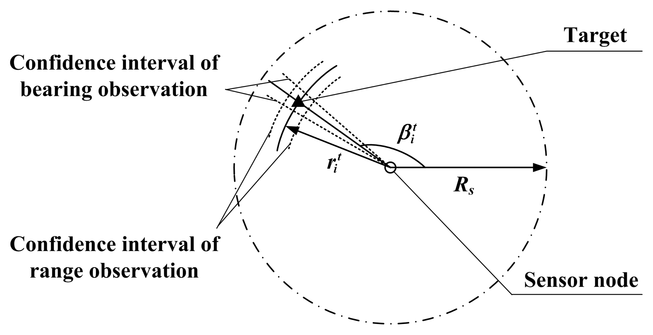
It is assumed that each sensor node equips two kinds of sensors, one pyroelectric infra-red (PIR) sensor and one omni-microphone sensor. Sensor nodes obtain the bearing observations of the target with the PIR sensors, while the range observations of the target are produced by the omni-microphone sensors. For each sensor node, it is assumed that the two sensors have the same sensing range Rs. Then the sensing function of a single sensor node is shown in Figure 2.
In Figure 2, the coordinates of the sensor node and target are denoted by (xi, yi) and (xtarget, ytarget) respectively. Then the true bearing angle is calculated as:
and the true range value is calculated as:
Both sensors have zero-mean and Gaussian error distribution. The standard deviation of bearing and range observations is σβ and σr respectively, which is related to the confidence interval of bearing and range observations. The observations produced by the sensor node i are:
where the wβ and wr are the corresponding Gaussian white noise.
2.3. Energy model
Basic sensor node architecture consists of the embedded sensors, A/D converter, a processor with memory and the radio frequency (RF) circuits. For the scalability of energy consumption in WSN, all the components of sensor node are supposed to be controlled by an operation system, such as microOperating System (μOS) [1]. Thereby, shutting down or turning on any component is enabled by device drivers in the specified application of WSN. Here, system-level energy consumption optimization can be performed according to the target motion information potentially.
During sensor node operation, four main parts of energy consumption source are considered: processing, sensing, reception and transmission. The processing energy is spent by the processor with memory. It is assumed that when the processor is active it has constant power consumption. The embedded sensors and A/D converter are adopted as there is any sensing task, and the corresponding power consumption is a constant. For wireless communication, the reception and transmission energy is derived from the RF circuits. As radio signal attenuation in the air is related with the distance of propagation, the free space propagation model [18] is adopted, which can be expressed as:
where Lp is the path loss, D is the propagation distance, and λs is the wavelength of signal.
When the reception portion is turned on, the sensor node keeps listening to the wireless channel or receiving data. Thus, the power consumption of reception portion is assumed to be constant. For the transmission portion of RF circuits, the transmission amplifier has to achieve an acceptable magnification. Therefore, when sensor nodes i transmits data to sensor node j, the power consumed by transmission portion is calculated as [19]:
where rd denotes the data rate, α1 denotes the electronics energy expended in transmitting one bit of data, α2 > 0 is a constant related to the transmission amplifier energy consumption, di,j is the Euclidean distance between the two sensor nodes. As the operation system can manage the components of sensor node, the energy consumption is adjustable according to different sensing situations.
With the stated basic models, collaborative sensing and adaptive estimation approaches will be exploited for the target tracking problem.
3. Collaborative Sensing and Adaptive Estimation in Target Tracking Problem
As mentioned in Section 2.2, each sensor node has a sensing range for target detection. Due to the redundancy of sensor node deployment in WSNs, the target can be detected by a group of sensor nodes simultaneously. Thus, the observations of these sensor nodes are merged for higher detection accuracy. The data from multiple sensor nodes, including bearing and range observations, is utilized to localize the target. In this way, collaborative sensing is achieved by maximum likelihood estimation. Moreover, the sink node constructs the forecasting model with the historical target trajectory. Time series analysis is employed for adaptive estimation of target position. Here, a differencing operation and the EMD approach represent the time series of target position by stationary components, which are forecasted by ARMA model respectively.
3.1. Target localization with multi-sensor fusion
It is assumed that the coordinates of target is (xtarget, ytarget) at one sensing instant of WSN. Meanwhile, the target can be detected by Ns sensor nodes, of which the coordinates are {(xi,yi) | i =1, 2, ⋯, Ns} . According to Section 2.2, these sensor node can produce the bearing observations βi and range observations ri, where i =1,2,⋯, Ns . For sensor node i, the matrix representation of observation equation can be derived from Equation (6) and (7):
where X = [xtarget, ytarget]T is the true target position, Γi =[βi,ri]T is the observation vector, the observation matrix is denoted as:
Wi is the observation error vector, N means the normal distribution function, and
With the observation of the sensor node i, the likelihood function of the true target position X is calculated as:
A suitable measure for the information contained in the observations can be derived from the Fisher information matrix (FIM) [20]. The FIM for the observations of sensor node i is calculated as:
where E represents the expected value.
According to Equation (13), we have:
where hi,1 = tan−1((ytarget − yi)/(xtarget − xi)), hi,2=[(xtarget − xi)2+(ytarget − yi)2]1/2. Then,
where Δxi = xtarget − xi, Δyi = ytarget − yi and
is the Euclidean distance between the true target position and sensor node i as presented in Equation (5).
is the estimation error covariance matrix, which defines the Cramer-Rao lower bound (CRLB). To localize the target with higher accuracy, we should extract the information from the all the observations { Γi | i = 1, 2, ⋯, Ns}. The FIM for all the observations is calculated as:
According to the estimation error covariance matrix J−1, the root mean square error (RMSE) Le is taken as the target location error, which is calculated as:
where trace is a function computing the sum of matrix diagonal elements.
In this way, the target can be localized by maximum likelihood estimation after gathering the observations from the sensor nodes. The location accuracy is reflected by Le.
3.2. Time series analysis for target position forecasting
It is assumed that the sink node keeps Nt points of the historical target trajectory {Yk | k = 1, 2, ⋯, Nt}. ARMA model is a widely-used model for the forecasting of future values. ARMA model is adopted here to forecast the target position YNt+1 due to its outstanding performance in model fitting and lightweight computational cost. Here, one direction of the target motion {Yk | k = 1, 2, ⋯, Nt} is taken for discussion.
The ARMA model contains two terms, the autoregressive (AR) term and the moving average (MA) term [21]. In the AR process, the current value of the time series yk is expressed linearly in terms of its previous values {Yk−1, yk−2, ⋯, yk−p} and a random noise ak. This model is defined as a AR process of order p, AR(p), which can be presented as:
where {ϕi | i=1,2⋯, p} are the coefficients of AR model. In the MA process, the current value of the time series yk is expressed linearly in terms of current and previous values of a white noise series {ak, ak−1, ⋯, ak−q}. This noise series is constructed from the forecasting errors. This model is defined as a MA process of order q, MA(q), which can be presented as:
where {θi | i = 1, 2, ⋯, q} are the coefficients of MA model.
The backshift operator B is introduced here, which is defined as:
and consequently
The backshift operator is not a number, but rather a symbol that denotes shifting of the time subscript.
Then, the AR process can be written as:
while the MA process can be written as:
where
In the autoregressive moving average process, the current value of the time series yk is expressed linearly in terms of its values at previous periods {yk−1, yk−2, ⋯ yk−p} and in terms of current and previous values of a white noise {ak, ak−1, ⋯, ak−q}. The order of the ARMA process is selected by both the oldest previous value of the series and the oldest white noise value at which yk is regressed on. For this ARMA of order p and q, ARMA(p, q), it can be written as:
There is an assumption for ARMA process that the time series for analysis should be stationary, that is, the mean of the time series and the covariance among its observations are not time-varied. According to the target model, the process is non-stationary, so the series should be transformed to a stationary process be the model construction. This can be often achieved by a differentiation process. The first-order differencing of the original time series is defined as:
For the high-order differentiation, we have:
After the d -order differentiation of yk, the autoregressive integrated moving average (ARIMA), ARIMA(p, d, q), can be constructed as:
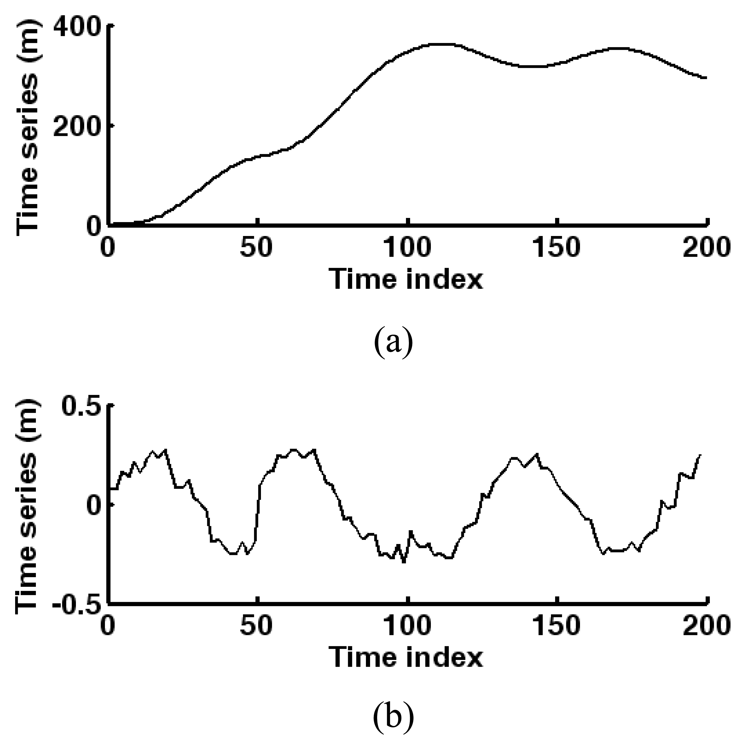
For instance, time series is simulated for one direction of target trajectory. As shown in Figure 3, the time series is generated according to Section 2.1, where the sensing period T is assumed to be 0.5 s. In Figure 3(a), there are 200 historical points of the target trajectory. The lost information of the original time series will be larger when the order of differencing increases. Therefore, the differentiation order d is set as 2. Then the time series after differentiation is shown in Figure 3(b). It can be seen that this series is basically stationary.
However, further processing of the time series is performed in order to obtain more stationary time series for forecasting. Here, EMD is introduced to decompose the time series into a set of stationary time series, called intrinsic mode functions (IMFs). More importantly, the IMFs can reflect the inherent variation mode in the time series, including stochastic components and a trend component.
EMD is a general nonlinear, non-stationary signal processing method, first proposed by Huang [22]. The major advantage of EMD is that the basis functions are derived directly from the signal itself. Hence, the analysis procedure is adaptive.
For each IMF, there are two definitive requirements: (1) the numbers of its extrema and zero-crossings are equal or differ at most by one; (2) it is symmetric with respect to local zero mean. The decomposition process is performed as follow:
- a)
- Identify all the maxima and minima of .
- b)
- Generate its upper and lower envelopes and with cubic spline interpolation.
- c)
- Calculate the point-by-point mean from upper and lower envelopes as:
- d)
- Extract the detail as:
- e)
- Check the properties of ek. If it meets the definitive requirements, an IMF is derived and the residual is:Otherwise, replace with ek
- f)
- Repeat Steps a) to e) until the residual satisfies the stopping criterion.
At the end of this process, the time series can be expressed as:
where m is the number of IMFs and
denotes the final residue series. {Ck,i | i = 1, 2, ⋯, m} denotes the set of IMFs, which are stationary and nearly orthogonal to each other.
Here, the number of IMFs m is specified as the stopping criterion. In WSN, the EMD process is started on the sink node. After the first IMF is extracted, the residue series is transferred to a sensor node with available computation resource, where the sensor node is selected randomly. Also, this sensor node forwards the residue series the nearest sensor node with available computation resource when the next IMF is obtained. Repeat this process until the decomposition is accomplished. In this way, the IMF and the final residue series are assigned among the sink node and a group of sensor nodes.
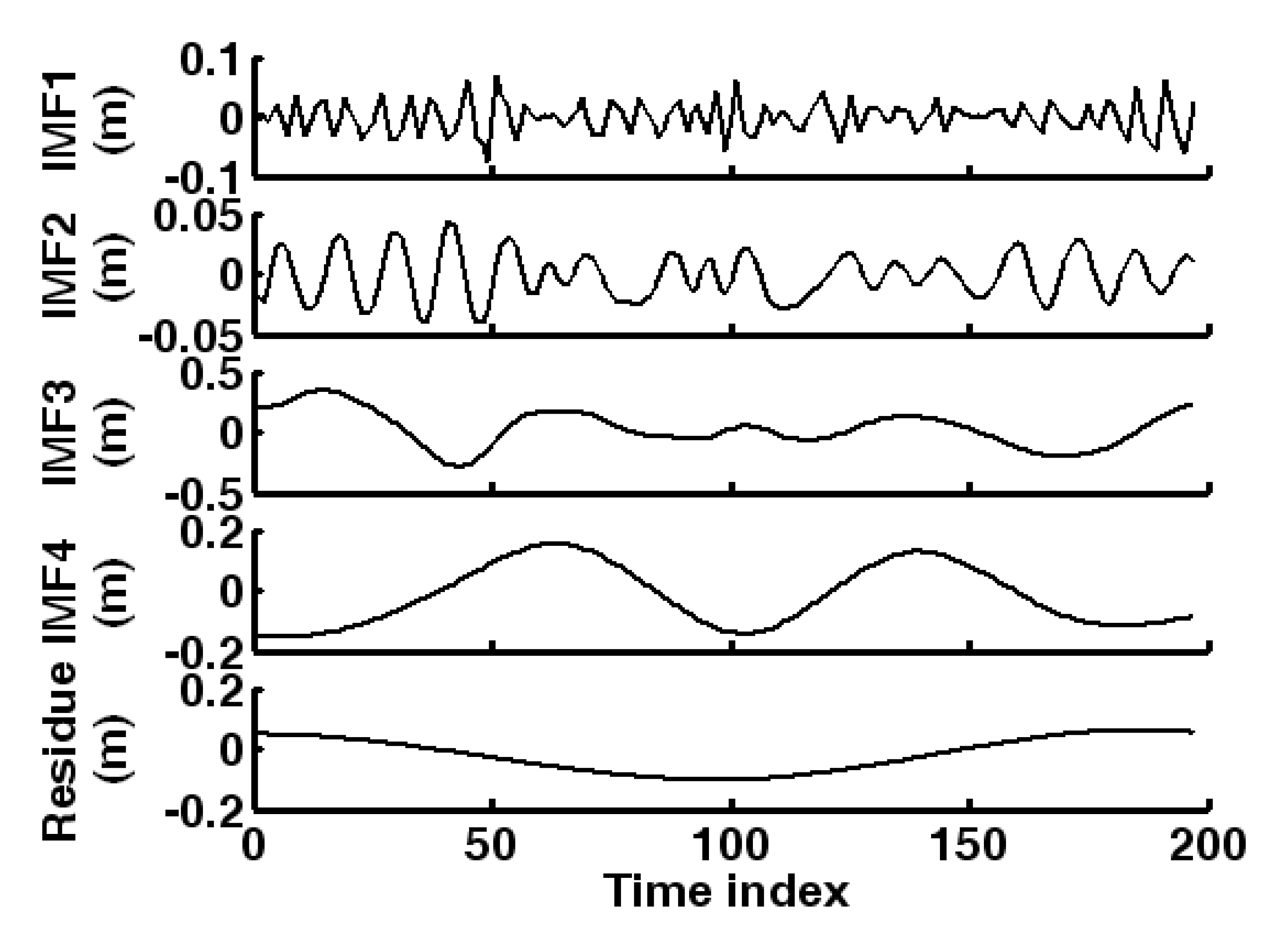
For the time series in Figure 3(b), the EMD process is implemented. To reduce computation cost and the decomposition error, the number of IMFs is set as 4. The decomposition results are shown in Figure 4, where the 4 IMFs and one final residue series is presented. Each IMF reflects different variation mode of the time series, so corresponding models are constructed separately. To determine the order of ARMA model, the patterns of autocorrelation function (ACF) and partial autocorrelation function (PACF) are analyzed.
For time series {zk}, ACF is defined as:
where is E means the expected value and l denotes the number of lags. PACF can be obtained by Yule-Walker equation [23]. Table 1 represents the patterns in the theoretical ACF and PACF of stationary time series, which is utilized to determine the order of model.
Taking the IMF1 in Figure 4 for example, its ACF and PACF are presented in Figure 5. According to Table 1, we choose the model AR(6). In the same way, models are chosen for all the IMFs and the final residue series. It is found that each component can be described by an AR model.
As mentioned earlier, the sink node and a group of sensor nodes maintain the components. Then, the AR(p) models can be constructed in a distributed manner.
For any time series {zk | k = 1, 2 ⋯, N}, the method of least square estimation is adopted to determine the coefficients of AR(p) [24]. A linear equation can be acquired as follow:
where Z1 = [zp+1 zp+2 ⋯ zN]T, and
Besides, B = [ϕ1 ϕ2 ⋯ ϕp]Tis the coefficient vector, A = [ap+1 ap+2 ⋯ aN]T is the noise vector. Here, {ϕ | i = 1, 2, ⋯, p} are the coefficients of AR model and {ai | i = p+1, p+2, ⋯, N} are previous values of a white noise series.
Then the least square estimation of coefficients is:
With the constructed AR(p) model, forecasting can be performed on the sink node and sensor nodes. The estimation value is calculated as:
where is E means the expected value. The forecasted results on the sensor nodes are forwarded back along the former path to the sink node, where the total result is obtained by calculating the sum of all the component results. Because the data amount is limited and the sensor nodes are close to each other, this part of energy consumption for communication is ignored.
In this way, both directions of the target position can be forecasted adaptively. Since the forecasted target position for the next sensing period is available, related energy-efficient organization will be implemented in WSN.
4. Energy-efficient organization method
With the forecasted target position, sensor nodes can be set to sleep when there is no sensing task. Due to the redundancy of sensor node deployment, the WSN performs probability awakening in a distributed manner to enhance the scalability of the energy consumption. Moreover, the routing scheme of data reporting is optimized by ACO for energy efficiency.
4.1. Distributed sensor node awakening
According to Section 2.3, sensor nodes can shut down its components if necessary. Thereby, sensor node awakening is considered with the forecasted target position. To prolong the lifetime of WSN, we exploit a sensor node awakening approach, where the mode transition of sensor node is scheduled and probability awakening is considered.
First, five operation modes of sensor node is defined as follow:
- (1)
- Sleep. It has the lowest power consumption as all the components are inactive. Only the timer-driven awakening is supported, that is, the processor component can be awakened by its own timer.
- (2)
- Idle. Only the processor component is active in this mode. All the other components can be controlled by the operation system.
- (3)
- Sense. The processor and sensor components are active. In this mode, sensor nodes can acquire the target observations.
- (4)
- Rx. The processor is working and the reception portion of RF circuits is turned on. Sensor nodes can receive request or data.
- (5)
- Rx & tx. The processor is active while both the reception and transmission portions of RF circuits are turned on. Sensor nodes can receive and transmit information.
Then, sensor node awakening strategy can be exploited according to the defined operation modes. Figure 6 illustrates the operation mode transition in distributed sensor node awakening approach according to the forecasted target position. Each sensor node controls its operation modes separately.
For a sensor node in idle mode, if there is no target in its sensing range, it will get into rx mode. Thus, the broadcasting information of the target position can be obtained from the sink node. Note that this target position is the target position estimation forecasted in the last sensing period. That is because the target localization is not accomplished yet while the sensor node should go to sleep as soon as possible. Then sensor node goes to sleep mode with the estimated sleep period number. If the sensor node in idle mode detects any target, it gets into sense mode for data acquisition. After that, the data is transmitted for data fusion in the rx & tx mode. Then, the forecasted target position is acquired. Also, the sensor node which finishes the sensing task goes to sleep mode adopting the estimated sleep period number.
Here, the estimation approach of sleep period number will be discussed. For each sensor nodes, define the shortest distance to the WSN boundary as dmin. Then, the sleep time can be estimated as:
where T denotes the sensing period, Rs is the sensing range of sensor node, ra is a random number in the interval (0,1], vmax is the maximum target velocity, and Δt is the prolonged sleep time which is a random number. γ is a parameter for adjusting the probability of sleep time prolonging. When any target gets into the sensing field, the Euclidean distance between the forecasted target position and the sensor node is denoted by dtarget′. If dtarget′ < dmin, then dtarget = dtarget′; otherwise, dtarget= dmin.
Thereby, WSN maintain standby for any new target getting into it. When there is a target in the sensing field, the sensor nodes which are far away from the target will go to sleep. The sleeping sensor nodes are awakened on time when there is potential sensing task.
In addition, the redundancy of sensor node deployment is utilized to prolong the sleep time. For the sensor nodes, the probability of prolonging the sleep time obeys exponential distribution, which is determined by the probability awakening parameter γ. The sleep period number can be calculate as fl(tsleep /T), where fl is the rounding operation.
The sensor node awakening situation around the target is that illustrated in Figure 7. The sensor nodes which are farther from the target ought to wake up in a later sensing period. The potential task range in the k-th period is the circle with radius Rs + kvmaxT while the potential task range in the (k+1) -th period is the circle with radius Rs + (k+1)kvmaxT. Here, k is the sensing period index from the current sensing period. Instead of awakening all the sensor nodes between the two circles, the probability awakening approach selects a set of sensor node randomly.
With the estimated sleep period number, sensor node can go to sleep mode to save the operation energy. Meanwhile, the awakening probability for potential task is adjustable to reduce redundancy observations.
4.2. Dynamic routing with ant colony optimization
When there is a target in the sensing field, a group of sensor nodes goes into the sense mode at each sensing instant. The observations produced by these sensor nodes should be transferred to the sink node for collaborative sensing. As these sensor nodes are close to each other, data transmission is enabled in one pair of sensor nodes at a time to avoid collisions in the communication. Therefore, a routing problem is considered as follows:
- (1)
- The index of sensor nodes with observations is denoted by {1, 2, ⋯, na};
- (2)
- (3)
- A optimal path {λ(1), λ(2), ⋯, λ(na)} should be found, where λ(i) ∈ {1, 2, ⋯, na}. At the beginning, sensor node λ(1) transmits its observations to sensor node λ(2). Then the data is forwarded and integrated along the path. The sensor node λ(na) can localize the target by data fusion in the end. If i ≠ j, then λ(i) ≠ λ(j). The minimization objective function is:
In this way, the observations of sensor nodes can be merged step by step on the path and the last sensor node will obtain the final target localization result. This result is then reported to the sink node. As it only includes the coordinates of the target, the communication cost is ignored.
It is assumed that the sink node maintains the awakening information of sensor nodes. Therefore, the optimization of routing scheme can be performed by the sink node. ACO is adopted to find the optimal path, where a society of artificial ants is modeled [25]. In addition to the cost measure, each edge has also a desirability measure τi,j, called pheromone, which is updated at run time by artificial ants. Each ant generates a complete tour by choosing the sensor nodes according to a probabilistic state transition rule. Ants prefer to move to sensor nodes which are connected by short edges with a high amount of pheromone. Once all the ants have completed their tours a global pheromone updating rule is applied. A fraction of the pheromone evaporates on all the edges, and then each ant deposits an amount of pheromone on edges which belong to its tour in proportion to how short its tour was. The process is then iterated. The state transition rule used by ant system is called a random-proportional rule. It gives the probability with which ant k in sensor node i chooses to move to the sensor node j as follow [26]:
where τi,j is the pheromone, δi,j is the inverse of the cost measure ρi,j,
is the set of sensor nodes that remain to be visited by ant positioned on sensor node i, and g (g > 0) is a parameter which determines the relative importance of pheromone versus distance. In Equation (43), the pheromone on edge (i, j) is multiplied by the corresponding heuristic value δi,j. In this way, the choice of edges which have a greater amount of pheromone is preferred. The global updating rule is implemented as follows. Once all ants have built their tours, pheromone is updated on all edges according to
where
0 < αt < 1 is a pheromone decay parameter, Lk is the length of the tour performed by ant k, and ma is the number of ants. Pheromone updating is intended to allocate a greater amount of pheromone to shorter tours. New pheromone is deposited by ants on the visited edges. Meanwhile, the pheromone is evaporated. The pheromone updating formula simulates this procedure. Finally, the edge which receives the greatest amount of pheromone is regarded as the optimal path.
5. Experimental Results
In this section, the efficiency of collaborative sensing, adaptive estimation and energy-efficient organization will be analyzed with simulation experiments.
5.1. Experimentation platform
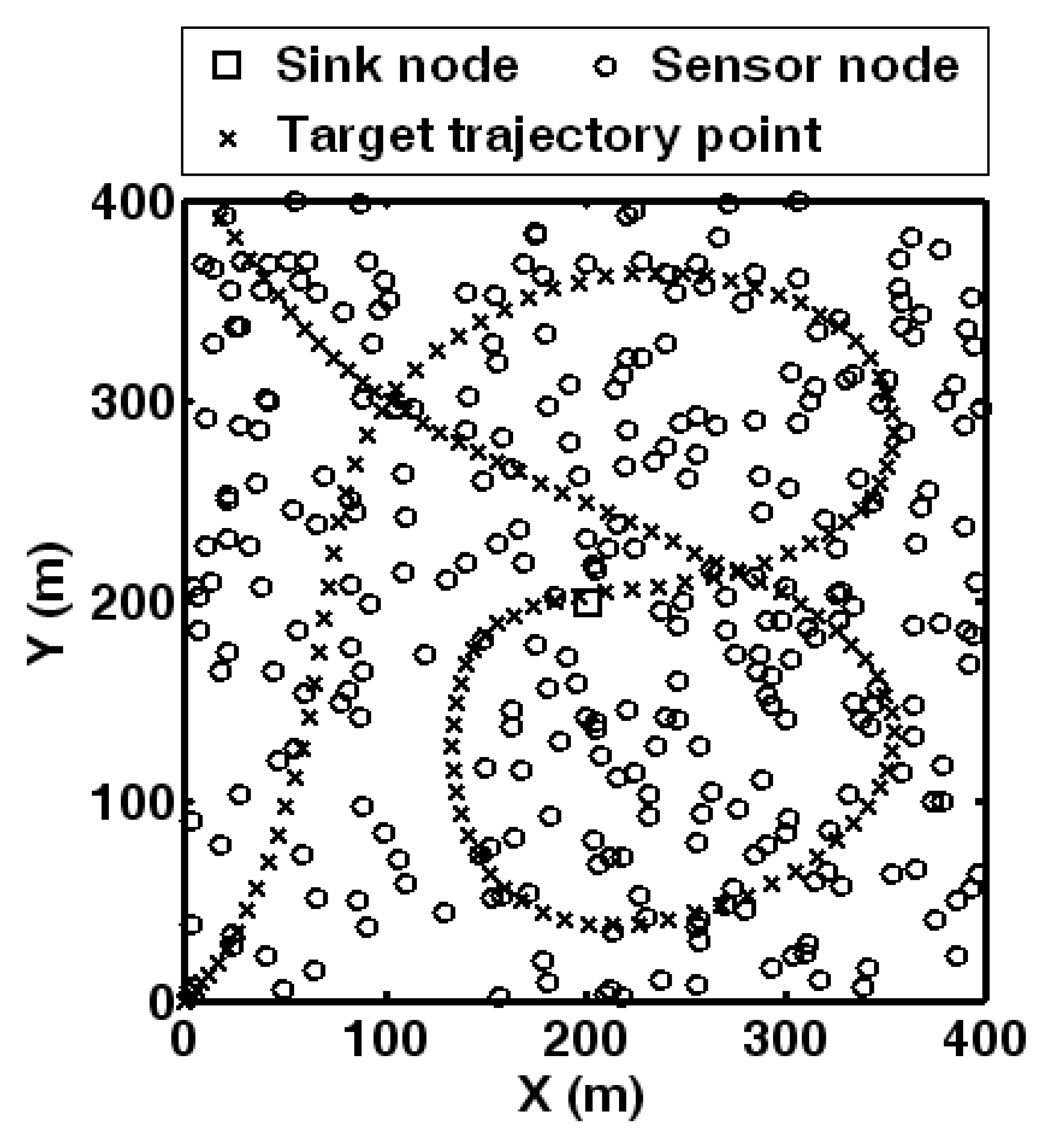
It is assumed that the sensing field of WSN is 400 m × 400 m, in which 300 wireless sensor nodes are deployed randomly. The sensing period T is set as 0.5 s. Deployment of WSN and the target trajectory is given in Figure 8. The acceleration of target is modeled according to Section 2.1. The trajectory involves different moving situations, so this scenario can represent the generalization of tracking problem. For the target trajectory, there are 150 points, the maximum acceleration amax is set as 8 m/s2 and the maximum velocity vmax is set as 30 m/s.
According to Section 2.2, each sensor node has the sensing range Rs = 40 m. The standard deviation of bearing observations is σβ = 2° while that of range observations is σr = 1m. In Section 2.3, the power consumption of sensor node components is set as typical value. The power consumption of the processor is 25mW; the power consumption of the embedded sensors and A/D converter 15 mW; the power consumption of reception portion is 25mW. Besides, the parameters in Equation (9) are set as: α1 = 500 nJ/bit, α2 = 5 nJ/(bit·m2) and rd = 1 Mibt/s. The basic power consumption for inactive processor component is 5 mW. According to Section 4.1, the power consumption of the five modes is presented in Table 2. As mentioned in Section 2.3, Ptx is the energy consumed by transmission portion.
During each sensing period, it is assumed that the time for staying in each mode is δt = 20 ms. Then, the power consumption of WSN in the each sensing period can be calculated as:
where T is the sensing period and k is the sensing period index. P(i,k)denotes the power consumption of sensor node i in the k-th sensing period. Moreover, the total energy consumption of WSN after nT sensing periods can be calculated as:
Among the total energy consumption, the energy consumed by transmission portion is related with the propagation distance of radio signal. For WSN, this part of energy consumption is defined as transmission cost, while the other part of energy consumption is defined as operation cost. Simulations of communication network will be performed with Opnet Modeler, which is a simulation platform for communication network and distribution system. It is assumed that the data amount of observations is 1KB for each sensor node. Three kinds of models are adopted in simulations: mobile target, wireless sensor node and sink node.
5.2. Target tracking experiments
The target tracking procedure with energy-efficient organization is simulated. As presented in Equation (40), the probability of prolonging the sleep time is determined by the probability awakening parameter γ. Here, it is assumed that γ approaches positive infinity so that sleep time prolonging is disabled in the distributed sensor node awakening. Sleep time prolonging by probability awakening will be studied separately later. Thus, all the sensor nodes that have potential sensing task will wake up on time.
Utilizing the target trajectory in Figure 8, the sensor nodes with the target in the sensing range acquire the bearing and range observations in each sensing period. The sink node finds the optimal routing scheme by ACO. Thereby, the observations are forwarded and fused hop by hop. The last sensor node on the path reports the final target localization result to the sink node. With the historical target positions, the sink node performs time series analysis. EMD and ARIMA model is adopted to forecast the target position in the next sensing instant. Hence, sensor node can estimate the sleep period number in a distributed manner based on the forecasted target position during the next sensing period. This process is repeated in the target tracking procedure.
First, the efficiency of collaborative sensing is discussed. For sensing performance comparison, we consider the situation that only the closest sensor node for the target acquires the observations. In this situation, the bearing and range observations of single sensor node is available and the related target location error can be derived from Equation (16). Figure 9 compares the target location error with collaborative sensing and single sensor node. It can be seen that the target location error of collaborative is much lower than that of single sensor node. Thus, the sensing performance is enhanced by the collaborative sensing, which provides more reliable results for the target position estimation stage. Then, the target position forecasting performance of time series analysis is studied. In each sensing period, the known target trajectory in the x and y directions forms two set of time series. It is assumed that target localization in the beginning 5 s can be guaranteed by boundary sensor node. As stated in Section 3.2, differentiation and EMD are used to process the original time series.
After experimental analysis, the differentiation order d is set as 2 while the IMF number m is set as 4. The order p of AR model for IMF1, IMF2, IMF3, IMF4 and the final residue series is set as 5, 4, 3, 4 and 3 respectively. This forecasting task is distributed among the sink node and 4 sensor nodes. Also, another situation is considered for comparison, in which the target position is forecasted without EMD. In other words, the time series after differentiation is forecasted by AR model in this situation. The order of AR model is set as 6. The way of selecting these parameters has been described in Section 3.2.
For the time series after differentiation, the forecasting error with and without EMD is compared in Figure 10. In x and y direction, the forecasting error is smaller utilizing the times series analysis with EMD. That is because the components obtained by EMD are more stationary and can reflect the inherent modes of target motion better. Then, the target position forecasted results are presented in Figure 11. Here, the error from target localization is involved in the total target position forecasting error. It can be seen that the time series analysis with EMD approximate the true trajectory of target better. The accuracy of target position forecasting will affect the following organization so that it is related with the sensing performance and energy efficiency.
With the distributed target position forecasting, the energy efficiency of the energy-efficient organization can be investigated. The sensor nodes estimate the sleep period number and go to sleep in a distributed manner according to Section 4.1. Thereby, the operation cost of WSN is optimized. In each sensing period, all the sensor nodes which can detect the target wake up. In order to minimize the transmission cost, ACO algorithm is utilized for routing.
According to Equation (46), the power consumption of WSN is calculated. As mentioned in Section 5.1, the operation and transmission costs are discussed. Figure 12(a) illustrates the total power consumption curves of WSN, including operation and transmission cost. Meanwhile, a general organization approach is considered for comparison. In the general organization procedure, all the sensor nodes wake up every sensing period. According to the distance from the sink node, all the detecting sensor nodes forward their observations step by step. It starts on farthest sensor node and ends on the closest sensor node. Accordingly, the total power consumption curves of WSN are presented in Figure 12(b). The operation and transmission costs are both lower in the target tracking with energy-efficient organization.
With the power consumption curves presented in Figure 12, Table 3 gives the energy consumption of the organization approaches utilizing Equation (47).
In Table 3, the relative reduction of energy consumption is calculated as:
where
and
denote the energy consumption of WSN with general organization and energy-efficient organization, respectively. Compared with the general organization approach, 11.4% operation cost and 54.6% transmission cost is saved by the energy-efficient organization approach.
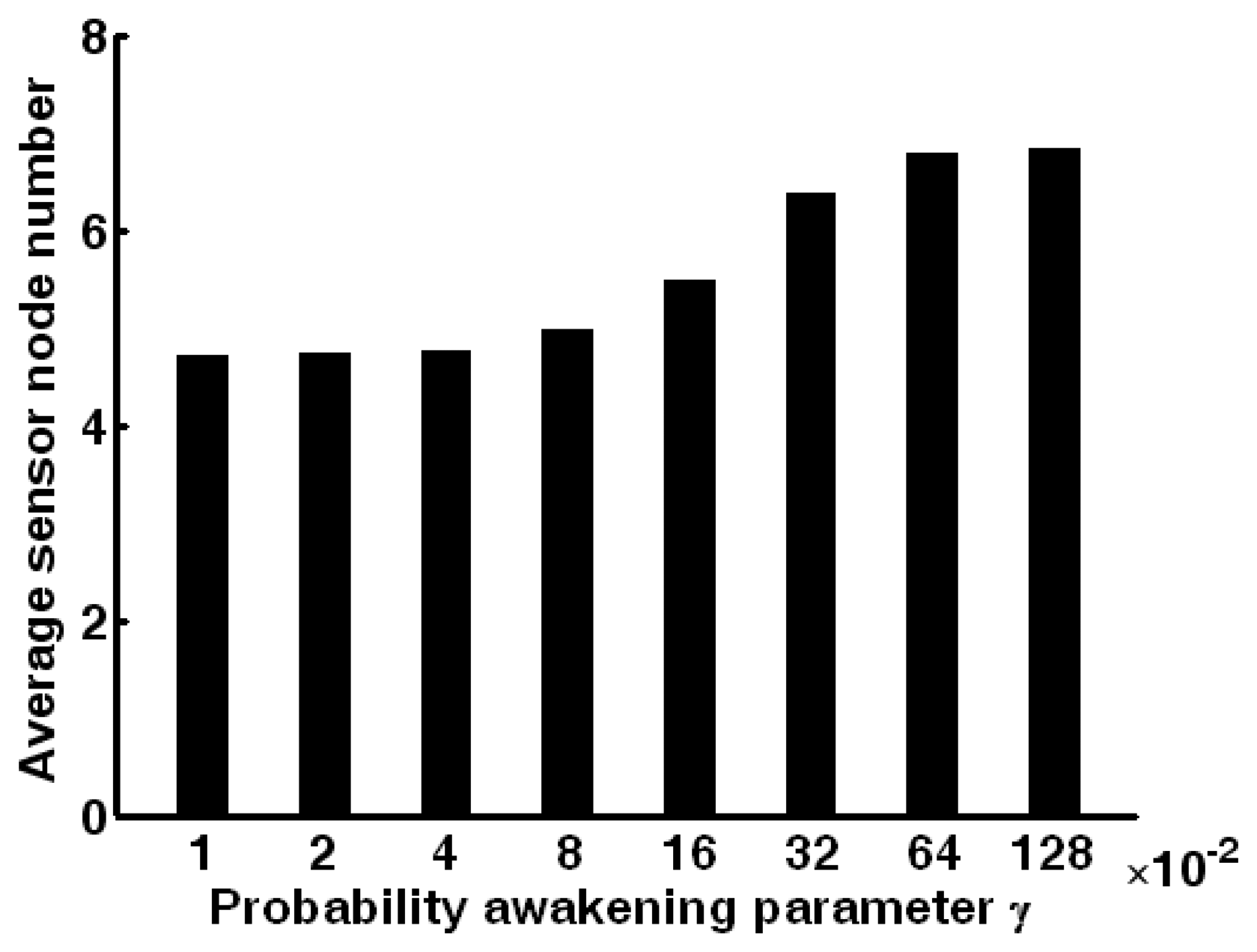
Moreover, the efficiency of the probability sleep prolonging is discussed in the distributed sensor node awakening. According to Equation (40), the probability awakening parameter γ can be specified to prolong the sleep time of sensor nodes. In other words, part of the sensor nodes which have potential sensing task in the corresponding sensing period will keep sleeping for the extension time. The sensor nodes have an extension time Δt with probability exp(−γΔt). Here, Δt is a random number in the interval [0 s,5 s]. A group of sensor nodes will be awakened for target detection during each sensing period. Adjusting the probability awakening parameter γ, the average number of sensor nodes available for target detection in one sensing period is presented in Figure 13. With smaller parameter γ the average number of detecting sensor nodes turns less. When γ exceeds 0.64, the average sensor node number becomes a constant. It is the maximum number of detecting sensor nodes that can be provided by WSN.
Considering the collaborative sensing accuracy, the cases in which the average number of detecting sensor node exceeds 5 is analyzed. According to Equations (46) and (47), the total energy consumed during target tracking can be calculated adopting different probability awakening parameter γ. Table 4 gives the total energy consumption of WSN with γ set as 0.08, 0.16, 0.32 and 0.64. The power consumption is lower with smaller γ. Thus, additional energy saving of WSN can be obtained by choosing a proper γ.
The experiments studied the energy efficiency of target tracking. Collaborative sensing enhances the target localization accuracy. Time series analysis based on EMD approximates the target trajectory well. Besides, the energy-efficient organization achieves energy saving. Moreover, the probabilistic in sensor node awakening leads to extra energy saving.
6. Conclusions
Considering the energy constraints of target tracking in WSN, this paper proposes an energy-efficient organization method based on collaborative sensing and adaptive target estimation. Sensor nodes which are equipped with bearing and range sensors utilize the maximum likelihood estimation for data fusion. Hence, targets can be localized by collaborative sensing while the localization error is evaluated utilizing FIM. A sink node maintains the historical target positions, with which the target position in the next sensing instant is estimated. The time series of target trajectory is processed by differentiation and EMD. Thereby, the inherent variation modes can be obtained, which are forecasted by the ARMA models. The future target position is derived from the forecasted results and is adopted to organize the sensor nodes for sensing. Here, the energy-efficient organization method includes the distributed sensor node awakening and adaptive routing scheme. Sensor nodes can go to sleep when there is no target in its sensing range and it can be awakened once there is potential sensing task. Besides, probabilistic awakening is introduced to prolong the sleep time of sensor nodes. ACO algorithm is employed to optimize the path of data transmission. Experiments of target tracking verify that target localization accuracy is enhanced by collaborative sensing of the sensor nodes, while the forecasting performance is improved by combining ARMA model with EMD. More importantly, the energy efficiency of WSN is guaranteed by the distributed sensor awakening and dynamic routing. In Section 2, the main contribution of this paper is the energy-efficient organization framework for target tracking as well as the forecasting and awakening approaches. For the future work, we may extend this method to other applications of WSN, such as target classification and environment surveillance. Also, the mobility of wireless sensor node could by investigate for further research.
Acknowledgments
This paper is supported by the National Grand Fundamental Research 973 Program of China under Grant No.2006CB303000 and the National Natural Science Foundation of China (No.60673176; No.60373014; No.50175056).
References and Notes
- Sinha, A.; Chandrakasan, A. Dynamic Power Management in Wireless Sensor Networks. IEEE Design and Test of Computers 2001, 18, 62–74. [Google Scholar]
- Lim, S. Adaptive power controllable retrodirective array system for wireless sensor server applications. IEEE Transactions on Microwave Theory and Techniques 2005, 53, 3735–3743. [Google Scholar]
- Tang, C.; Raghavendra, C.S. Power aware wireless sensor networks using tripwire detection and cueing. Proceedings of International Conference on System Sciences; 2005; pp. 1–10. [Google Scholar]
- Duh, F.B.; Lin, C.T. Tracking a maneuvering target using neural fuzzy network. IEEE Transactions on System, Man, and Cybernetics 2004, 34, 16–33. [Google Scholar]
- Wang, X.; Wang, S.; Ma, J. An improved particle filter for target tracking in sensor system. Sensors 2007, 7, 144–156. [Google Scholar]
- Payne, O.; Marrs, A. An unscented particle filter for GMTI tracking. Proceedings of IEEE Aerospace Conference; 2004; 3, pp. 1869–1875. [Google Scholar]
- Zhang, H. Optimal and self-tuning State estimation for singular stochastic systems: a polynomial equation approach. IEEE Transactions on Circuits and Systems 2004, 51, 327–333. [Google Scholar]
- Lin, Z.; Zou, Q. Cramer-Rao lower bound for parameter estimation in nonlinear systems. IEEE Signal Processing Letters 2005, 12, 855–858. [Google Scholar]
- Gabriel, R.; Patrick, F.; Paulo, G. Empirical mode decomposition, fractional Gaussian noise and Hurst exponent estimation. Proceedings of International Conference on Acoustics, Speech, and Signal Processing; 2005; 4, pp. 489–492. [Google Scholar]
- Zecchin, A.C. Parametric study for an ant algorithm applied to water distribution system optimization. IEEE Transactions on Evolutionary Computation 2005, 9, 175–191. [Google Scholar]
- Cardei, M.; Thai, M.T. Energy-efficient target coverage in wireless sensor networks. Proceedings of IEEE INFOCOM; 2005; pp. 1976–1984. [Google Scholar]
- Hohlt, B.; Doherty, L. Flexible power scheduling for sensor networks. Proceedings of International Symposium on Information Processing in Sensor Networks; 2004; pp. 205–214. [Google Scholar]
- Passos, R.M.; Coelho, C.J.N. Dynamic Power Management in Wireless Sensor Networks: An Application-Driven Approach. Proceedings of International Conference on Wireless On-demand Network Systems and Services; 2005; pp. 109–118. [Google Scholar]
- Du, X.; Lin, F. Efficient energy management protocol for target tracking sensor networks. IEEE International Symposium on Integrated Network Management 2005, 45–58. [Google Scholar]
- Wang, X.; Ma, J.; Wang, S.; Bi, D. Prediction-based dynamic energy management in wireless sensor networks. Sensors 2007, 7, 251–266. [Google Scholar]
- Wang, X.; Wang, S. Collaborative signal processing for target tracking in distributed wireless sensor networks. Journal of Parallel and Distributed Computing 2007, 67, 501–515. [Google Scholar]
- Rong, L.X.; Jilkov, V.P. Survey of maneuvering target tracking Part I: Dynamic models. IEEE Transactions on Aerospace and Electronic Systems 2003, 39, 1333–1364. [Google Scholar]
- Yao, Q.; Tan, S.K.; Ge, Y. An area localization scheme for large wireless sensor networks. Proceedings of IEEE Vehicular Technology Conference; 2005; pp. 2835–2839. [Google Scholar]
- Chhetri, A.S. Energy efficient target tracking in a sensor network using non-myopic sensor scheduling. Proceedings of International Conference on Information Fusion; 2005; pp. 558–565. [Google Scholar]
- Oshman, Y.; Davidson, P. Optimization of observer trajectories for bearings-only target localization. IEEE Transactions on Aerospace and Electronic Systems 1999, 35, 892–902. [Google Scholar]
- Broersen, P.M.T. Automatic identification of time-series models from long autoregressive models. IEEE Transactions on Instrumentation and Measurement 2005, 54, 1862–1868. [Google Scholar]
- Delechelle, E. Empirical mode decomposition: an analytical approach for sifting process. IEEE Signal Processing Letters 2005, 12, 764–767. [Google Scholar]
- Salami, M.J.E. Analysis of multiexponential transient signals using interpolation-based deconvolution and parametric modeling techniques. Proceedings of IEEE International Conference on Industrial Technology; 2003; 1, pp. 271–276. [Google Scholar]
- Biscainho, L.W.P. AR model estimation from quantized signals. IEEE Signal Processing Letters 2004, 11, 183–185. [Google Scholar]
- Liang, Y.C. An ant colony optimization algorithm for the redundancy allocation problem (RAP). IEEE Transactions on Reliability 2004, 53, 417–423. [Google Scholar]
- Dorigo, M.; Gambardella, L.M. Ant colony system: A cooperative learning approach to the traveling salesman problem. IEEE Transactions on Evolutionary Computation 1997, 1, 53–66. [Google Scholar]
Figure 1.
Energy-efficient organization framework for target tracking in WSN.
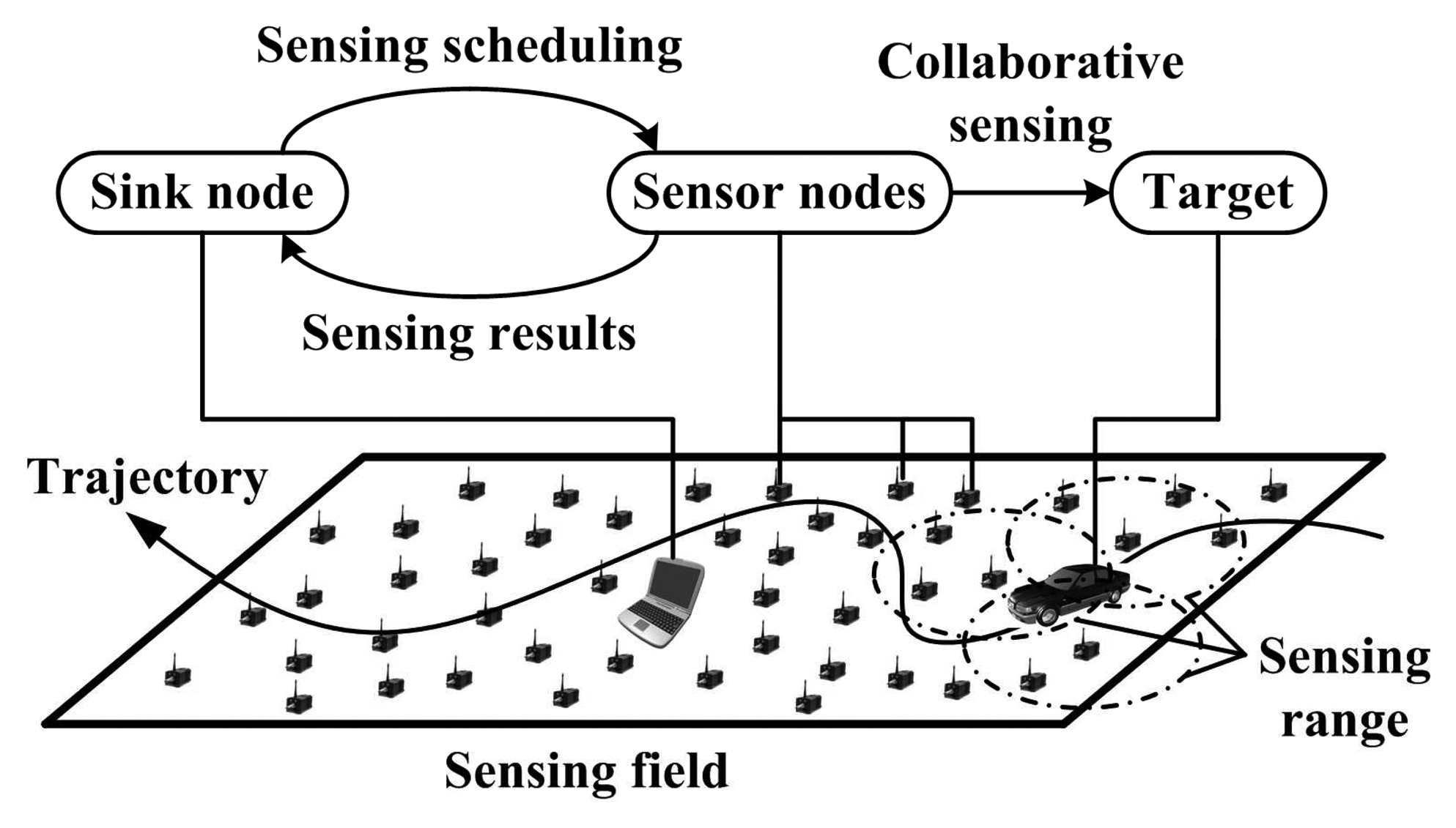
Figure 2.
Sensing function of a single sensor node.

Figure 3.
Simulated time series of target trajectory: (a) Before differentiation; (b) After differentiation.
Figure 3.
Simulated time series of target trajectory: (a) Before differentiation; (b) After differentiation.

Figure 4.
Decomposition results for the time series after differentiation.

Figure 5.
Analysis of ACF and PACF patterns: (a) ACF; (b) PACF.
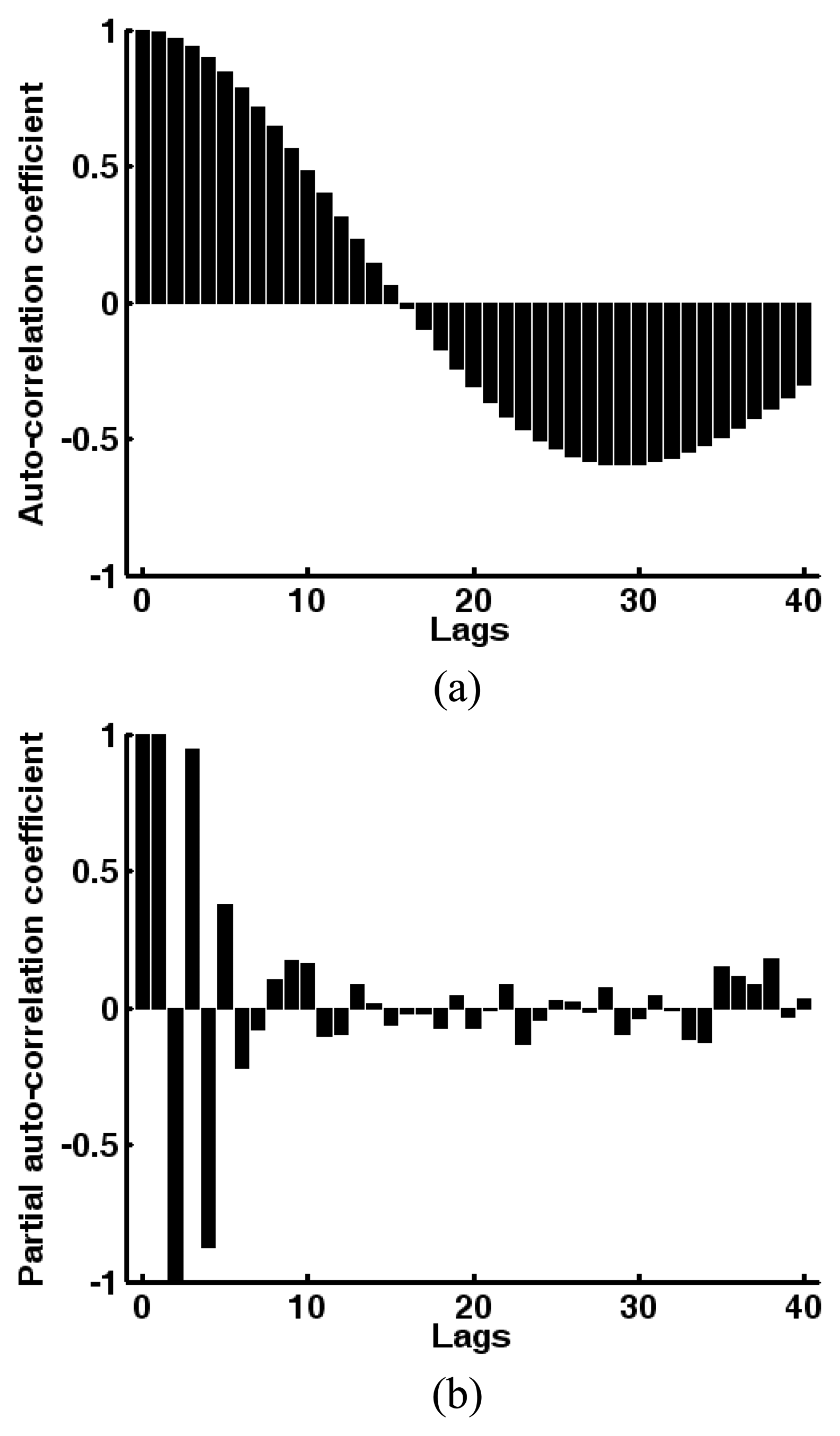
Figure 6.
Operation mode transition in distributed sensor node awakening approach according to the forecasted target position.
Figure 6.
Operation mode transition in distributed sensor node awakening approach according to the forecasted target position.
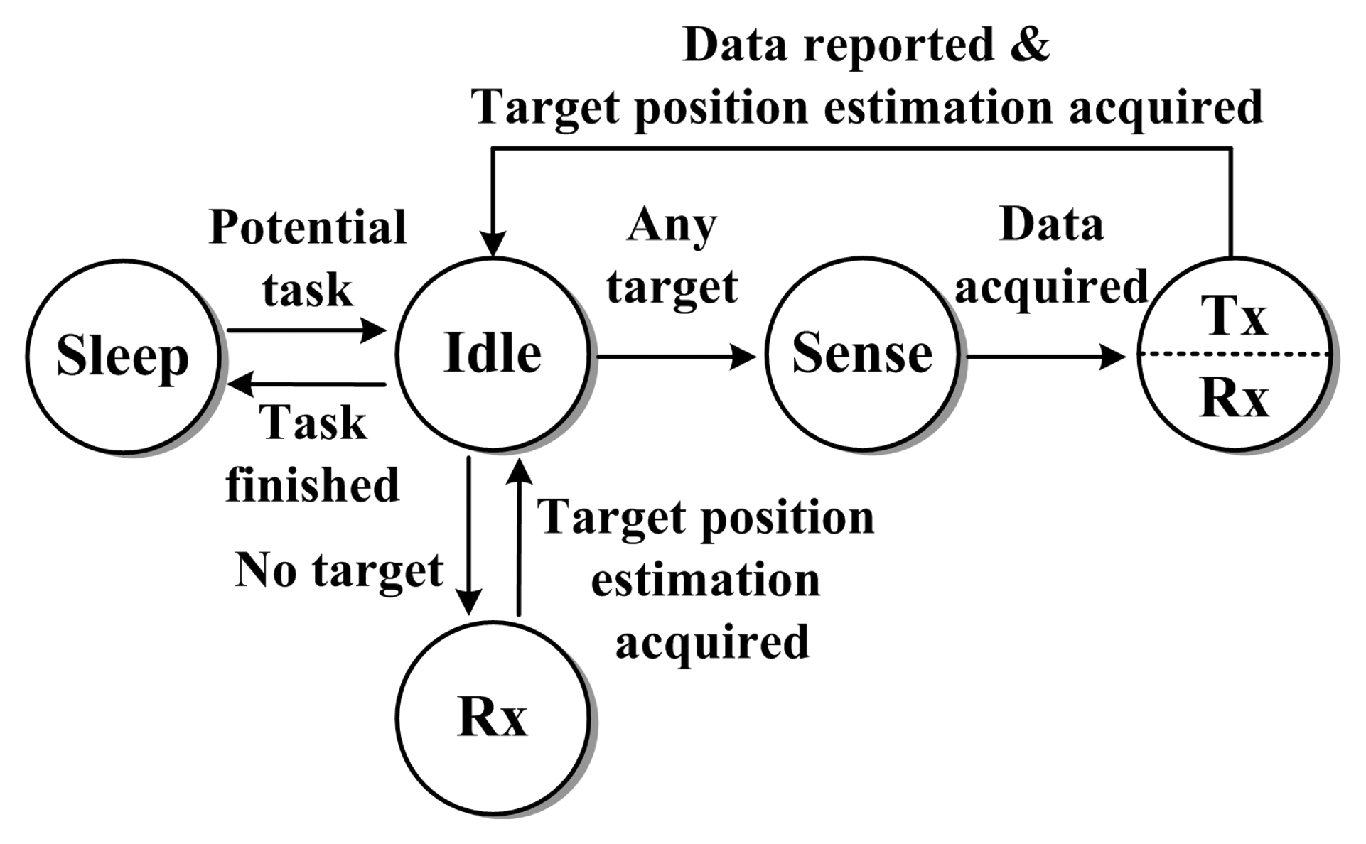
Figure 7.
Sensor node awakening when there is a target in WSN sensing field.
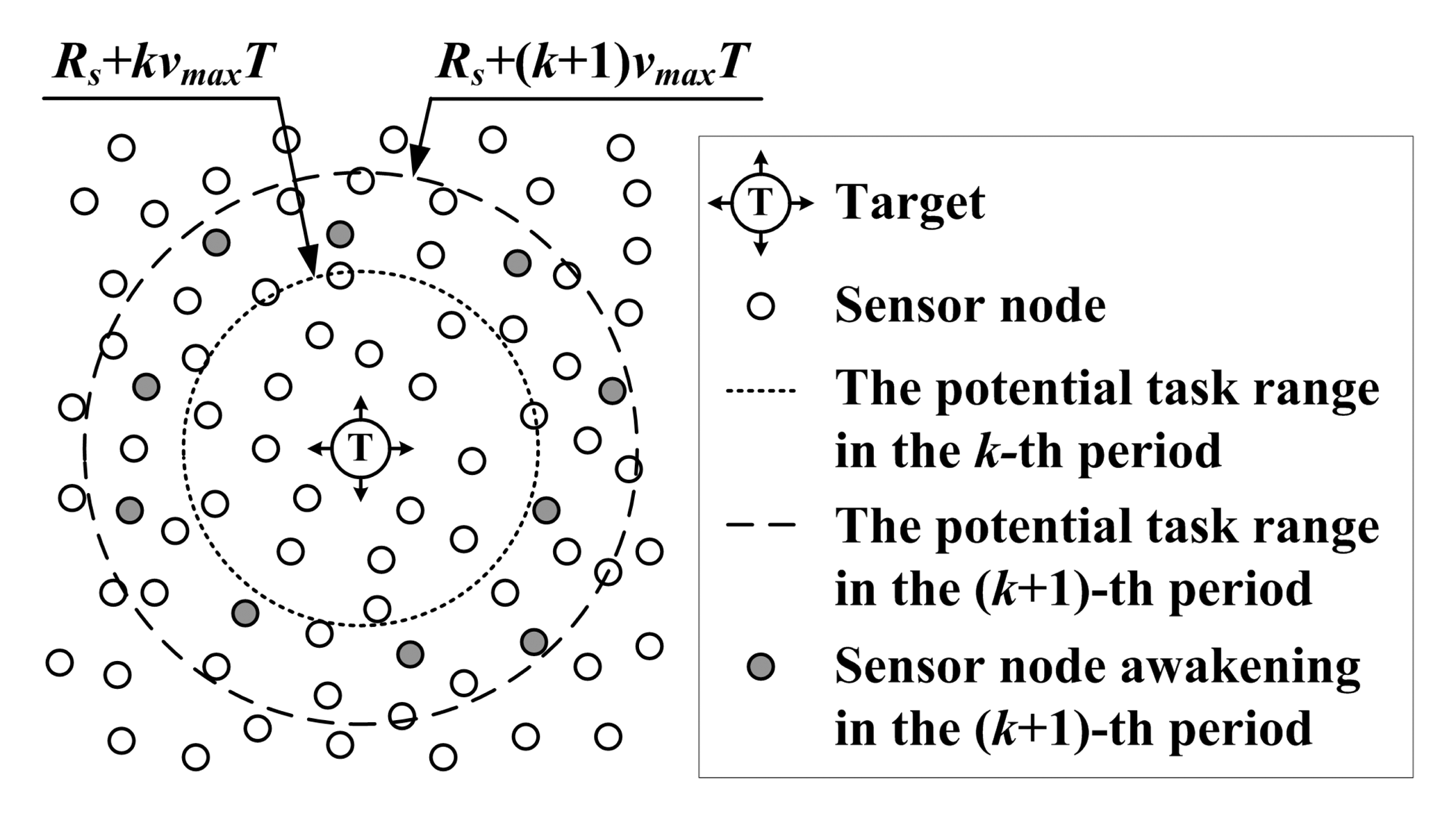
Figure 8.
Deployment of WSN and the target trajectory.

Figure 9.
Comparison of target localization error with collaborative sensing and single sensor node.
Figure 9.
Comparison of target localization error with collaborative sensing and single sensor node.
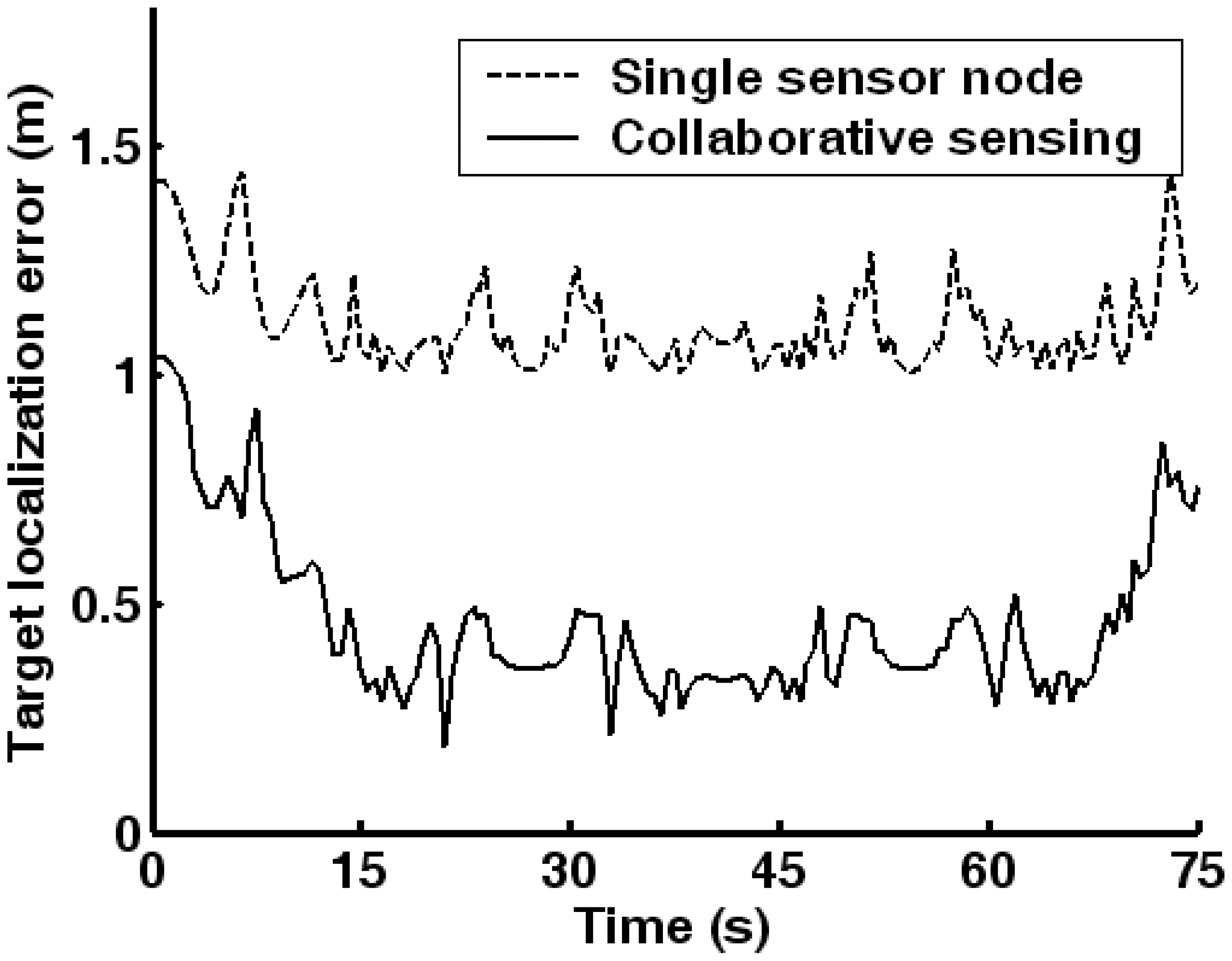
Figure 10.
Comparison of forecasting error with and without EMD for time series after differentiation: (a) X direction; (b) Y direction.
Figure 10.
Comparison of forecasting error with and without EMD for time series after differentiation: (a) X direction; (b) Y direction.
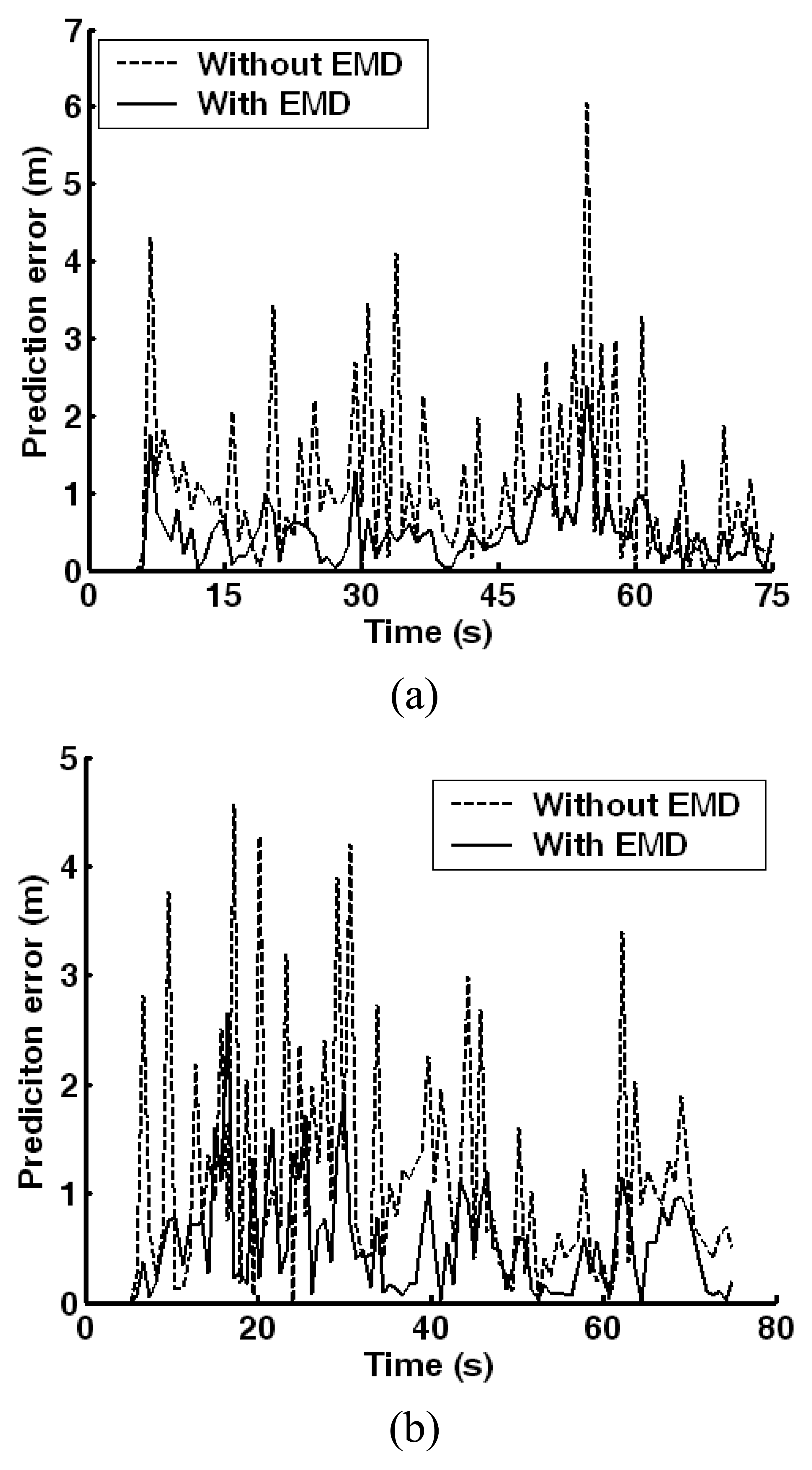
Figure 11.
Target position forecasted results utilizing time series analysis with and without EMD.
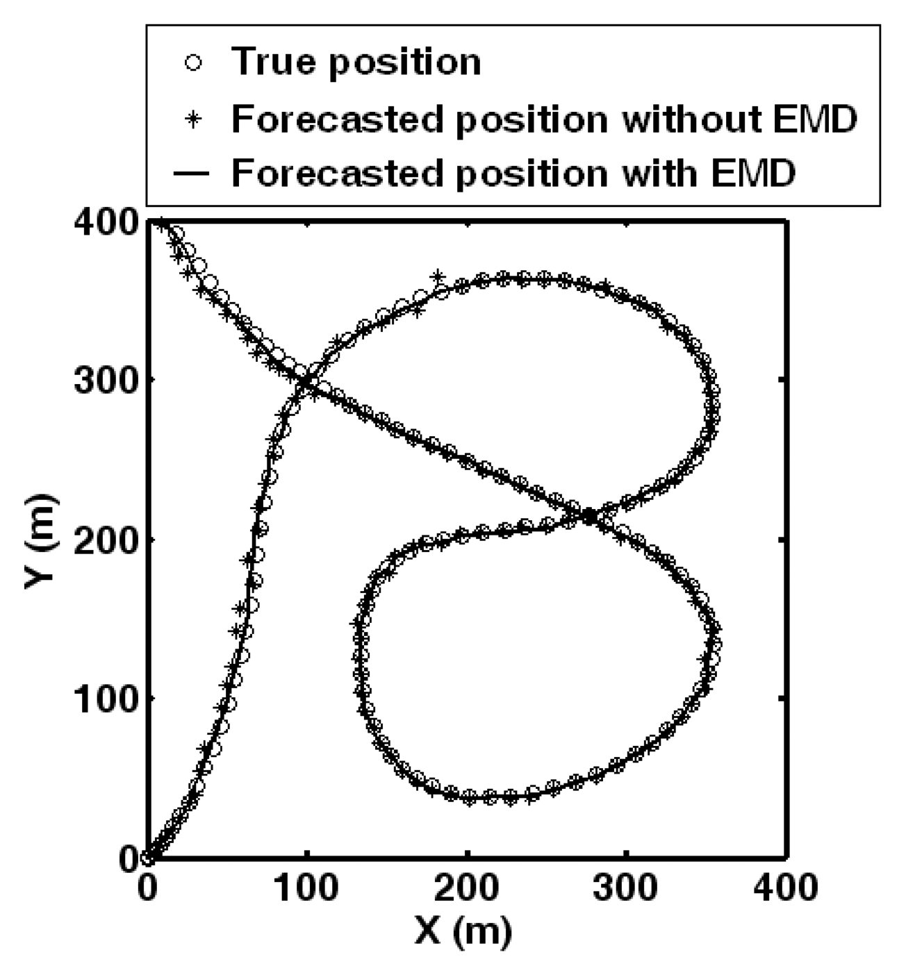
Figure 12.
Power consumption curves of WSN including operation and transmission cost: (a) Energy-efficient organization; (b) General organization.
Figure 12.
Power consumption curves of WSN including operation and transmission cost: (a) Energy-efficient organization; (b) General organization.
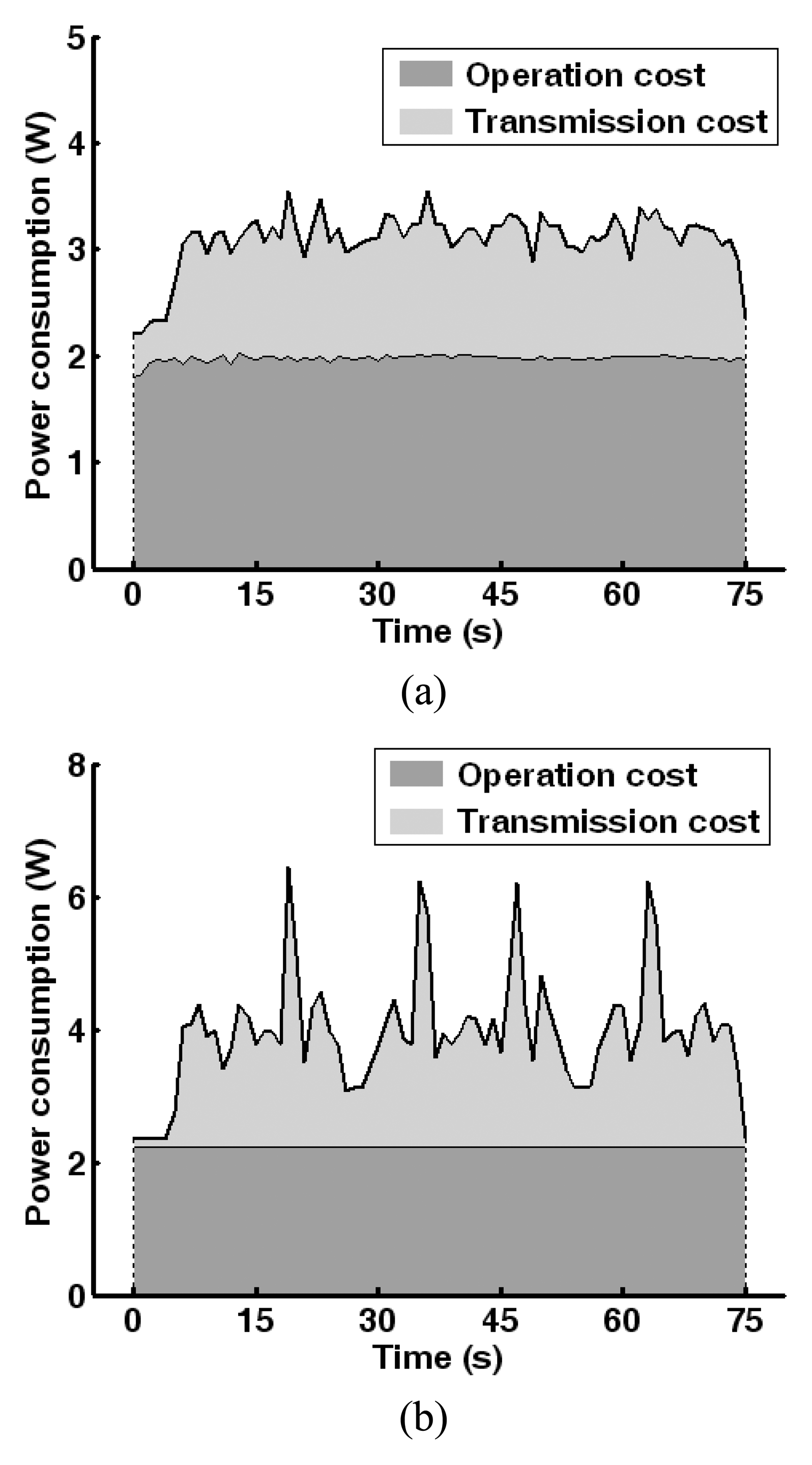
Figure 13.
Average number of sensor nodes available for target detection in one sensing period with different probability awakening parameter γ.
Figure 13.
Average number of sensor nodes available for target detection in one sensing period with different probability awakening parameter γ.

| Model | AR(p) | MA(q) | ARMA(p,q) |
|---|---|---|---|
| ACF | Exponential or sinusoidal decay to zero | Spikes cut off to zero after lag q | Exponential or sinusoidal decay to zero after lag q |
| PACF | Spikes cut off to zero after lag p | Exponential or sinusoidal decay to zero | Exponential or sinusoidal decay to zero after lag p |
| Mode | Power consumption (mW) |
|---|---|
| Sleep | 5 |
| Idle | 25 |
| Sense | 40 |
| Rx | 45 |
| Rx & tx | 45+Ptx |
| Cost type | Energy consumption (J) | Reduction (%) | |
|---|---|---|---|
| General organization | Energy-efficient organization | ||
| Operation | 167.4 | 148. 4 | 11.4 |
| Transmission | 132.4 | 84.1 | 36.5 |
| Total | 299.8 | 232. 5 | 22.4 |
| γ | 0.08 | 0.16 | 0.32 | 0.64 |
| Energy consumption (J) | 189.1 | 201.6 | 217.1 | 229.7 |
© 2007 by MDPI ( http://www.mdpi.org). Reproduction is permitted for noncommercial purposes.
Share and Cite
MDPI and ACS Style
Wang, X.; Ma, J.-J.; Wang, S.; Bi, D.-W. Time Series Forecasting Energy-efficient Organization of Wireless Sensor Networks. Sensors 2007, 7, 1766-1792. https://doi.org/10.3390/s7091766
AMA Style
Wang X, Ma J-J, Wang S, Bi D-W. Time Series Forecasting Energy-efficient Organization of Wireless Sensor Networks. Sensors. 2007; 7(9):1766-1792. https://doi.org/10.3390/s7091766
Chicago/Turabian StyleWang, Xue, Jun-Jie Ma, Sheng Wang, and Dao-Wei Bi. 2007. "Time Series Forecasting Energy-efficient Organization of Wireless Sensor Networks" Sensors 7, no. 9: 1766-1792. https://doi.org/10.3390/s7091766