Review

A Compact Laboratory Spectro-Goniometer (CLabSpeG) to Assess the BRDF of Materials. Presentation, Calibration and Implementation on Fagus sylvatica L. Leaves

1
Katholieke Universiteit Leuven, Dept. of Biosystems, M3-BIORES, Celestijnenlaan 200E, BE-3001 Leuven, Belgium
2
Katholieke Universiteit Leuven, Dept. of Computer Science, Celestijnenlaan 200A, BE-3001 Leuven, Belgium
3
ouncil for scientific and Industrial Research (CSIR) Natural Resources and the Environment – Ecosystems Earth Observation P.O.Box 395, 0001 Pretoria, South Africa
4
Katholieke Universiteit Leuven, Dept. of Land Management and Economics, Celestijnenlaan 200E, BE-3001 Leuven, Belgium
*
Author to whom correspondence should be addressed.
Sensors 2007, 7(9), 1846-1870; https://doi.org/10.3390/s7091846
Submission received: 2 August 2007 / Accepted: 6 September 2007 / Published: 7 September 2007
(This article belongs to the Special Issue Remote Sensing of Natural Resources and the Environment)

Abstract

:
The design and calibration of a new hyperspectral Compact Laboratory Spectro-Goniometer (CLabSpeG) is presented. CLabSpeG effectively measures the bidirectional reflectance Factor (BRF) of a sample, using a halogen light source and an Analytical Spectral Devices (ASD) spectroradiometer. The apparatus collects 4356 reflectance data readings covering the spectrum from 350 nm to 2500 nm by independent positioning of the sensor, sample holder, and light source. It has an azimuth and zenith resolution of 30 and 15 degrees, respectively. CLabSpeG is used to collect BRF data and extract Bidirectional Reflectance Distribution Function (BRDF) data of non-isotropic vegetation elements such as bark, soil, and leaves. Accurate calibration has ensured robust geometric accuracy of the apparatus, correction for the conicality of the light source, while sufficient radiometric stability and repeatability between measurements are obtained. The bidirectional reflectance data collection is automated and remotely controlled and takes approximately two and half hours for a BRF measurement cycle over a full hemisphere with 125 cm radius and 2.4 minutes for a single BRF acquisition. A specific protocol for vegetative leaf collection and measurement was established in order to investigate the possibility to extract BRDF values from Fagus sylvatica L. leaves under laboratory conditions. Drying leaf effects induce a reflectance change during the BRF measurements due to the laboratory illumination source. Therefore, the full hemisphere could not be covered with one leaf. Instead 12 BRF measurements per leaf were acquired covering all azimuth positions for a single light source zenith position. Data are collected in radiance format and reflectance is calculated by dividing the leaf cycle measurement with a radiance cycle of a Spectralon reference panel, multiplied by a Spectralon reflectance correction factor and a factor to correct for the conical effect of the light source. BRF results of measured leaves are presented.

1. Introduction

Research on reflectance of vegetation during the last 30 years has conclusively established that most of the Earth's surface is non-Lambertian. Any feature analysis, except the most simple and crude approximations, therefore must consider the non-Lambertian properties of earth elements and the importance of reflectance anisotropy [1]. This reflectance anisotropy is an intrinsic surface characteristic that affects all the terrestrial remote sensing measurements and is described physically in terms of the Bidirectional Reflectance Distribution Function (BRDF) [2].
The bidirectional reflectance property of vegetative earth surfaces results from factors such as the scattering process within the canopy layer, leaf angle distribution and orientation, thickness and size of leaves, crowns and their spatial distribution [3-5], as well as the underlying ground-soil properties such as roughness, color, and organic matter content [6]. Furthermore, not only the radiation transfer modeling community is interested in the BRDF of vegetation but also the computer graphics scientists [7-8]. There is a long tradition to represent surface reflection of any target in computers graphics by various models and a constant need exists to accurately represent and retrieve the BRDF of any surface including vegetation [9-11].
Several authors have reported significant work on BRDF measurement campaigns of vegetative surfaces either in the field [12-17] or in controlled laboratory conditions [18-25].
The few existing laboratory BRDF devices for vegetative materials have a restriction on the existing light incident angles, as well as the measured wavelengths. Brakke [20] used three incident light angles and measured a single wavelength, while Walter-Shea et al. [21] did the same for up to 1000 nm wavelengths. The goniometer of [23], though multi-angular and rapid, still measures the spectrum up to 950 nm, while similarly the one of [26] covers the electromagnetic spectrum in the region between 500 nm and 880 nm. In the cases that the wavelength and the viewing angles are not imposing any restrictions such as in the EGO/JRC goniometer, the acquisition time prohibits any vegetative material to survive under the light source, and the viewing area of the sensor is relatively large to focus exclusively on a leaf target. Moreover, for a Bidirectional Reflectance Factor (BRF), that means for a fixed source or sensor zenith angle, EGO/JRC goniometer covers the upper part of the hemisphere in 90 – 120 minutes [27]. The above mentioned issues, regarding also the geometric irregularity of plant canopies and the need for forest element BRDF data also in the infrared region of the electromagnetic spectrum, concluded the need of a new device that deals with existing disadvantages and mechanical restrictions whilst adding advantages such as the whole hyperspectral domain, the limited time of data acquisition and the fine steps in angular positioning.
In collaboration with the needs of the computer graphics science a Compact Laboratory Spectro-Goniometric device (CLabSpeG) was constructed to allow for an accurate measurement of the BRF of any material in a limited acquisition time, although we focus on measurements of vegetation elements. The implementation of the goniometer addresses the difficulties in capturing leaf reflectance properties while investigating practical considerations related to the instrument and the measured samples:
(i)
Geometric stability of the apparatus, velocity of the components, and deviation of the sensor field-of-view across the target.
(ii)
Stability, homogeneity, and conical illumination of the light source, consistency and repeatability of measurements, and the deviation of Spectralon from an ideal Lambertian reference panel.
(iii)
Water stress induced to the samples due to heat from the light source, and the irregularity of sample sizes compared to the field of view of the spectroradiometer.
In this paper the Compact Laboratory Spectro-Goniometric device (CLabSpeG) is presented with a description of the apparatus, the measurement and calibration protocol, and the assessment of the accuracy and preciseness of the BRDF and BRF retrievals. The methodology protocol is focused on leaf BRDF behavior and modeling, with primary research objectives to (i) represent the non-Lambertian state of leaf reflectance, (ii) investigate the differences in BRDF among different wavelengths and angular combinations and (iii) sum up practical considerations and issues that arise when vegetative BRDF data are acquired.

2. Theoretical background

The BRDF is defined as the ratio of the radiance Lr (W m-2 sr-1 nm-1), reflected in an outgoing direction (θr, φr) to the incident irradiance Ei (W m-2 nm-1) from a specific direction (θi, φi). BRDF is an intrinsic property of materials and in reality it can only be approximated by dividing measured radiances, Lr from small aperture solid angles by the hemispherical irradiance, Ei since an infinitesimally small sensor field of view is impossible to obtain [2].The mathematical expression of BRDF fr (sr-1) is:
f r ( θ i , ϕ i ; θ r , ϕ r ; λ ) = d L r ( θ i , ϕ i ; θ r , ϕ r ; λ ) d E i ( θ i , ϕ i ; λ )
where:
  • Lr = sensor radiance (W m-2 sr-1 nm-1),
  • Ei = hemispherical irradiance (W m-2 nm-1),
  • λ = wavelength (nm),
  • θii = source zenith and azimuth angles, respectively,
  • θrr = view zenith and azimuth angles, respectively.
  • fr values range theoretically from zero to infinity.
Hemispherical irradiance refers to the total irradiance incident on a target from any direction within the hemisphere (2π steridian solid angle). Ei is derived indirectly by integrating the reflected radiance, L, from a Spectralon sample over the hemisphere, in our case:
E i ( λ , θ i ) = 1 ρ ϕ r = 0 ϕ r = 2 π θ r = 0 θ r = π 2 L ( λ , θ r , ϕ r ) cos ( θ r ) sin ( θ r ) d θ r d ϕ r
where
  • ρ = hemispherical reflectance of sample.
Errors in estimating Ei can be introduced by the fact that the hemispherical reflectance of a Spectralon panel only approximately equals one and that a Spectralon is not a completely energy lossless material [28]. The Bidirectional Reflectance Factor (BRF), R, is defined as the ratio of radiance reflected from a surface into a specific direction to the reference radiance, Lref, reflected from an ideal lossless Lambertian reference surface measured under identical viewing and illumination geometry. When the bidirectional reflectance properties of a surface are measured, the measurement procedure usually follows the definition of the BRF [29]. An ideal Lambertian surface reflects the same radiance in all view directions and its BRDF is π-1. Thus, the BRF (unitless) of any surface can be expressed as its BRDF (sr-1) times π [30].
For a single direction illumination condition the BRF can be written as:
R ( θ i , ϕ i ; θ r , ϕ r ; λ ) = L ( θ i , ϕ i ; θ r , ϕ r ; λ ) L ref ( θ i , ϕ i ; θ r , ϕ r ; λ )
However, to take into account the non Lambertian reflection behavior of the Spectralon reference panel a correction factor Rref is required. Thus:
R ( θ i , ϕ i ; θ r , ϕ r ; λ ) = L ( θ i , ϕ i ; θ r , ϕ r ; λ ) L ref ( θ i , ϕ i ; θ r , ϕ r ; λ ) R ref ( θ i , ϕ i ; θ r , ϕ r ; λ )
where:
  • Rref = correction factor for the non-Lambertian reflection properties of the reference panel.
In laboratory conditions due to instrumentation issues of the illumination source and the sensor field of view, a single directional reflectance factor can not be obtained. Since our light source has a conical field of view, the resulted measured values produce the Biconical Reflectance Factor instead of the Bidirectional Reflectance Factor [30]. Thus the measured quantity is the Biconical Reflectance Factor (Conical-Conical Reflectance Factor, CCRF).
CCRF = R ( θ i , ϕ i , ω i ; θ r , ϕ r , ω r ; λ ) = ω r ω i f r ( θ i , ϕ i ; θ r , ϕ r ) L i ( θ i , ϕ i ) d Ω i d Ω r ( Ω r / π ) ω i L i ( θ i , ϕ i ) d Ω i
where ω is the solid angle and Ω = ∫ cosθdω∫∫cosθsinθdθφ is the projected solid angle of the cone. It should be noted that the CCRF contains in its expression all the cases describing reflectance quantities: for ω = 0 the integral is omitted and we obtain the directional reflectance, while for ω = 2π the hemispherical one [29-30].
The conical effect is corrected as described in [31] by considering the geometric configurations of the goniospectroradiometer following an inversion of the forward case (Eq. 6). Analytically, we assume that the signal observed by the detector, Φs, is proportional to the integral of the incoming radiation Li, weighted by the Bidirectional Reflectance Factor R over all locations (x, y) in the target reference plane and all possible illumination angles.
Φ s ( μ , μ 0 , ϕ , ϕ 0 ) x , y GIFOV R ( ( x , y ) , μ r ( x , y ) , μ i ( x , y ) , ϕ r ( x , y ) , ϕ i ( x , y ) ) × L i ( x , y ) , μ r ( x , y ) , μ i ( x , y ) r s 2 ( x , y ) dxdy
where:
  • Li = incoming radiance (W m-2 sr-1 nm-1),
  • R = Bidirectional Reflectance Factor,
  • μ = cosθ,
  • rs= the distance between the location (x,y,0) and the position of the sensor,
  • θ00 and θ,φ = nominal illumination and sensor angles, respectively.
The nominal angles correspond to the geometry of illumination and observation for the center of the reference point (0,0), illuminated from the center of the lamp, and observed from the center of the detector, respectively. The integral boundary is given by the rim of the ground instantaneous field of view (GIFOV). More details on the correction method and applied formulas are given in [31].

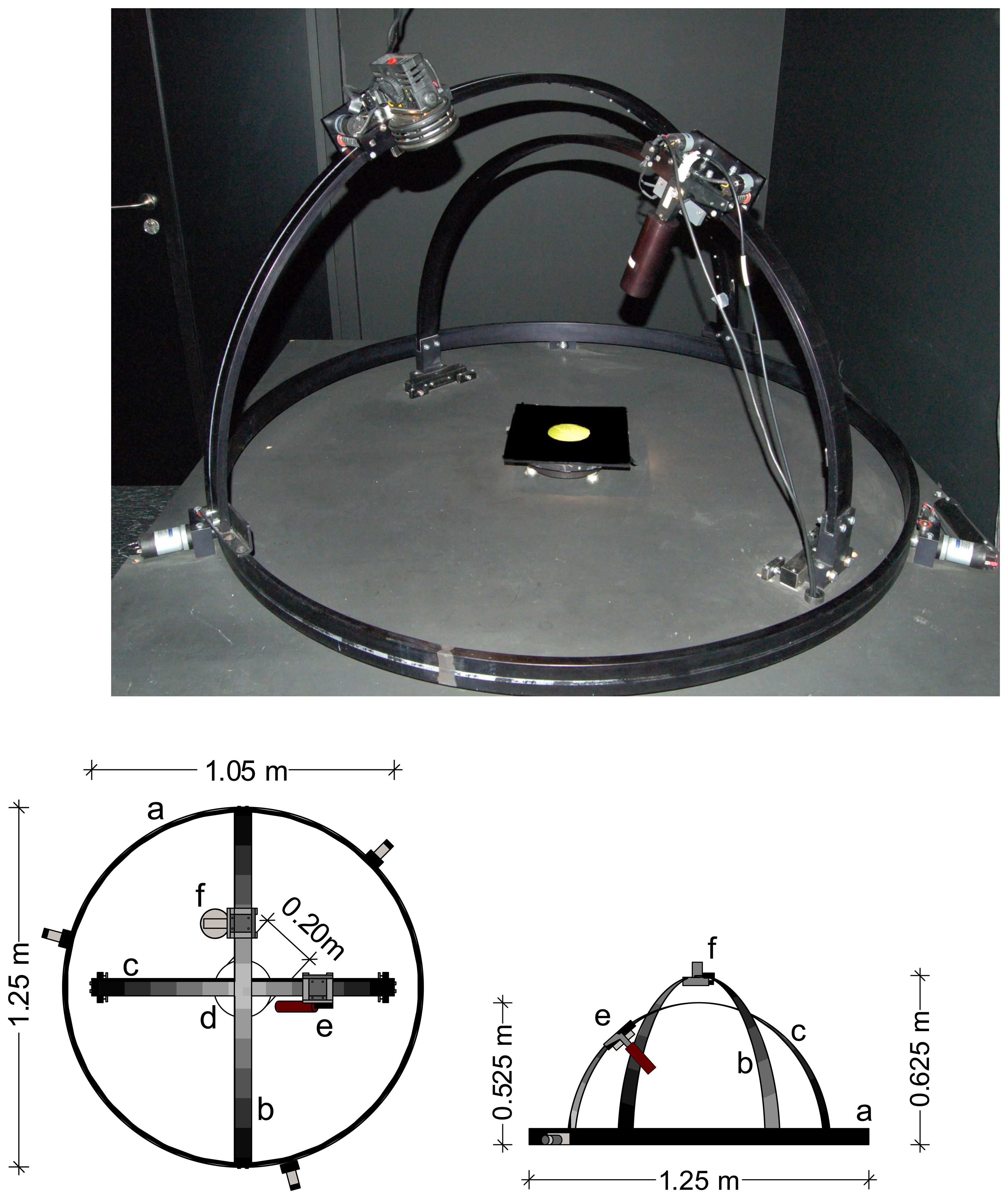
3. System Set up and Technical specifications

CLabSpeG is designed to measure the BRF of any material with special focus on vegetation elements of the size of a leaf, in a limited acquisition time and in hyperspectral mode. It consists of four major components, placed in a painted black laboratory to avoid any stray light effects. Figure 1 shows a picture and a schematic view of CLabSpeG.
  • A horizontal, circular black anodized aluminum rail ring of 1.25 m diameter for the azimuthal movement of the light source.
  • A vertical half-circular arc (diameter = 1.25 m) mounted on the horizontal rail, supporting the zenith movement of the light source.
  • A vertical stationary half-circular arc (diameter = 1.05 m) mounted inside both previous arcs on a black wooden table to support the zenith movement of the spectroradiometer.
  • A rotating stainless steel horizontal plate of 0.20 m diameter, placed in the centre of the apparatus, which enables the azimuthal movement of the sample holder.
The rings and arcs are 5 cm wide and 1.5 cm thick. The circular rail allows for azimuthal motion of the light source and rests on three 24 Volt precision motors, which support up to 200 Newton each and provide an angular resolution of 30°. The light source-supporting arc spans 180° in zenith having laser cut metal bolts at 5° increment. These bolts are recognized and engaged at each incremental position by a precision motorized chariot. Micro switches control the movement of the motors by providing position feedback for the controller software. However, the software is currently programmed for a 15° resolution in the zenith plane. The light source is mounted on the chariot with its optical axis aligned with the centre of the sample holder. The arc that supports the chariot carrying the fiber optic cable of the detector is similar in construction and has the same angular resolution covering 90° in zenith. Furthermore, light source and sensor are mounted sideways of the arcs so as to minimize shadow effects in the principal plane.
The rotating sample holder is driven by a precision motor that allows rapid rotations with an angular resolution of 30°. It also can be adjusted in the horizontal plane, upwards or downwards by up to 3 cm, so as to align the sample surface with the detector and light horizontal planes. This enables the instrument to obtain a full hemispherical coverage with a resolution of 30° in azimuth and 15° in zenith, which provides adequate angular resolution for capturing the BRDF of most natural and man-made surfaces [32].
Any sequence of positions can be programmed and executed from the controlling software and the apparatus captures the target reflectance following a repetitive pattern that delivers the BRF of the sample. Each measured reflectance is attributed with an arithmetic coded value that corresponds to a known angular configuration, given that the repetitive pattern is known.
The light source mounted on the apparatus is a tungsten halogen 50 W Ushio lamp, inside a Lowel assembly of 12.7 cm diameter. The lamp, which produces 1250 lumen, covers the electromagnetic spectrum in the region of 350 nm to 2500 nm and provides a sufficiently strong signal for the detector. The detector is an ASD Field Spec Pro JR. spectroradiometer that measures the wavelength range from 350 to 2500 nm using 3 detectors for the visible, near-infrared, and middle-infrared part of the spectrum, respectively. The spectral resolution is 3 nm in the visible and 30 nm in the infrared, with an associated sampling interval of 1.4 nm for the 350-1000 nm range and 2 nm for the 1000-2500 nm range. The ASD captures the full operating spectrum in 0.1 seconds and for each reflectance measurement an average of ten readings are used. The spectroradiometer software provides data per nanometer, using a cubic spline interpolation [33]. A one-meter fiber optic cable with a field of view of 1° is attached to the spectroradiometer and allows rapid and efficient positioning, without any bending of the cable, providing a footprint diameter from a distance of 0.35 m from the sample area of 0.025 m at nadir position.
The movement and positioning of the CLabSpeG components, as well as the operation of the spectroradiometer are remotely controlled by Labview software (V6.1, 2001). The system is able to operate both in manual mode, where the commands are given by the user, as well as in batch mode where the commands are read from a position file. This allows for full remote automation of measurements in a completely dark environment, while a camera monitors the measurement progress and a digital hydro-thermometer (OREGON Scientific) records room temperature and moisture. A roof-mounted mechanical balancer with a flexible steel cable ensures that continuous tension is kept on power cables so as not to interfere with the mechanical movement of the apparatus.
The total weight of CLabSpeG is less than 25 kg, while the light source weighs 700 g and the weight of the fiber optic cable is negligible. The compact nature of CLabSpeG results in accelerated measurements and full capture of BRDF characteristics of a target.
Data, via the spectroradiometer, are collected in radiance mode. The full measurement cycle is also performed for a Spectralon reference panel under the same geometrical configurations as those used for the samples. The reasoning behind this process is to correct for any asymmetry of the light source footprint on the target, by dividing the radiance of the sample with the equivalent radiance of the Spectralon at the same geometric position. This approach ensures that the amount of light incident to the sample holder is always the same for two corresponding measurements of sample and Spectralon. Consequently, errors resulting from the experimental setup such as illumination heterogeneity or detector footprint variations are likely to cancel since they occur for both the reference panel and target measurements in an equal way [27]. The division of the two radiance cycles provides the reflectance of the target at each sensor-light angle combination.
The total measurements for a full hemisphere cycle are 4356 given a zenith and azimuth resolution of 15° and 30° respectively and lasts 2 hours and 36 minutes while the acquisition time for a full BRF measurement (consisting from 66 positions) takes only 2.4 minutes.

4. Calibration

In our calibration protocol the geometric stability of the apparatus was evaluated in terms of angular stability and positional precision, velocity of the components, and deviation of the sensor field-of-view across the target. Furthermore, CLabSpeG was tested by evaluating the stability, homogeneity, and conicality of the light source. The consistency and repeatability of measurements, the target temperature over time, and the deviation from an ideal Lambertian Spectralon reference panel were also assessed.

4.1 Geometric Calibration

The geometric accuracy of the sensor field-of-view was tested using a laser sight as described by [34-35]. This was accomplished by moving the sight over the zenith arc that supports the spectroradiometer fiber optic while tracing the deviations of the laser spot from the centre of the sample holder. The observed deviations among the 6 zenith positions (0° to 75°) were smaller than 0.7 cm. The same procedure was followed for the azimuthal rotation of the sample holder where 12 positions were recorded on graphic millimeter paper, creating a circle of 2 cm diameter with a difference among them of 30° and maximum deviation of ± 2°. The angular positioning of the sensor and the light source is controlled via the stepping motors, with the use of the laser cut bolts, and the deviation is on the order of 0.01 degrees.

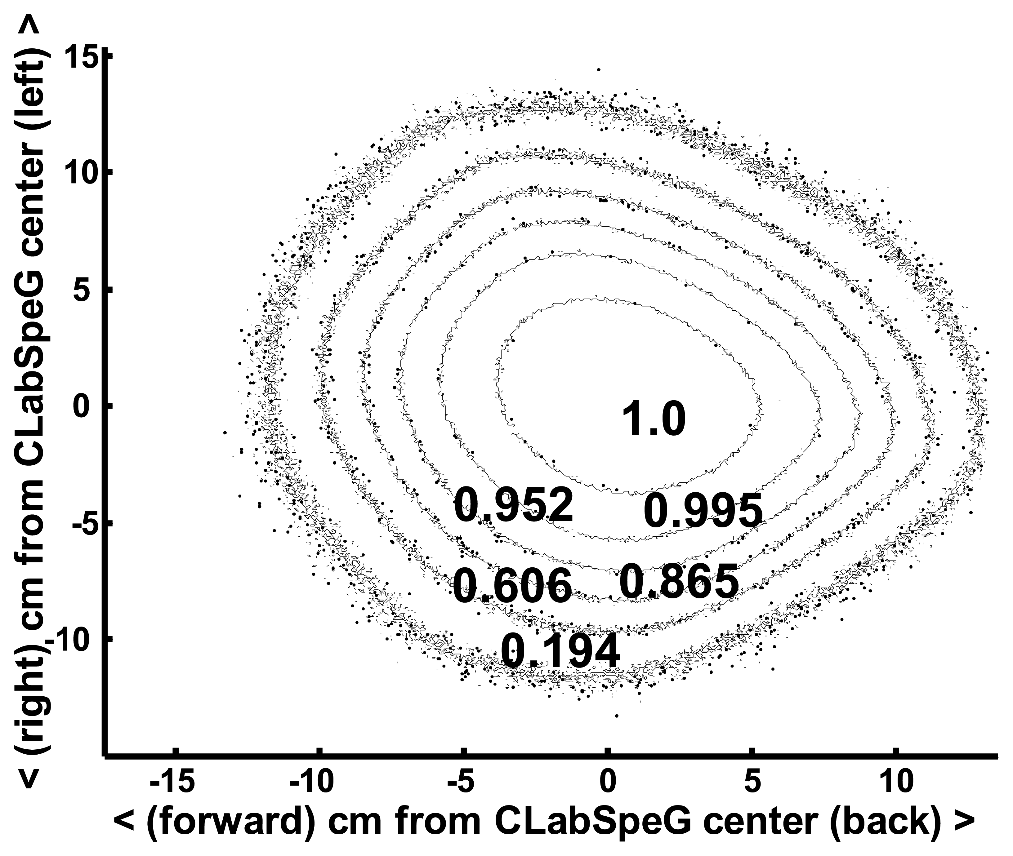
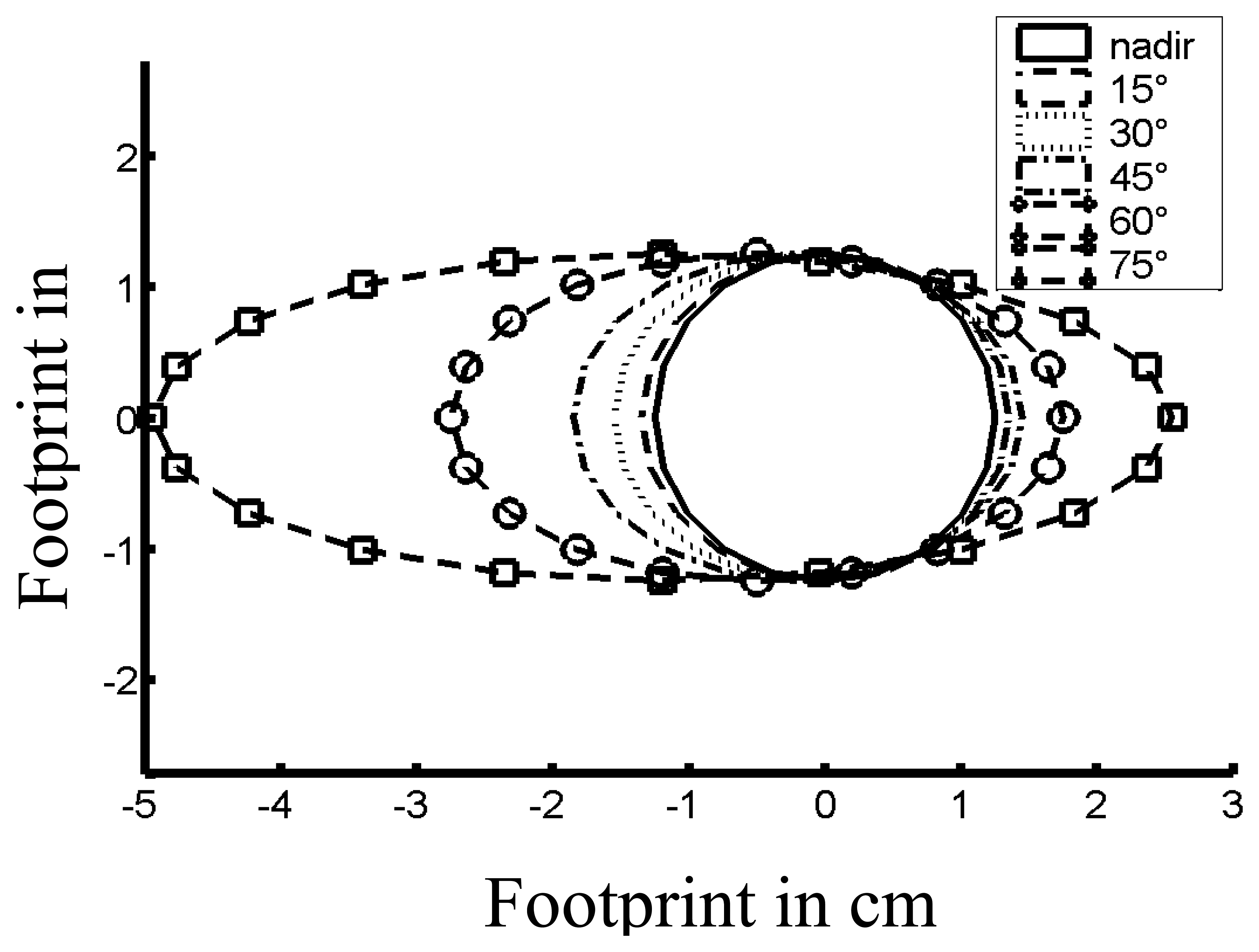
4.1.1 Ground Instantaneous Field Of View

The deviation of the sensor field-of-view across the target was examined by using a light pointer inside the 1° foreoptic. The footprint was recorded on millimeter paper for each of the 6 zenith positions. At nadir we have an almost circular footprint with 0.025 m diameter that becomes distinctively elliptical towards higher sensor zenith angles reaching a major half axis of 0.0375 m in 75°. It should be noted that with the use of a foreoptic the final footprint size includes also the diameter of the foreoptic itself. The changing footprint area of the sensor's field of view for various zenith angle positions is shown in figure 2.

4.2 Radiometric Calibration

For a relative calibration procedure (ratio of two measurements) several parameters were measured, such as the stability and homogeneity of the light source, target temperature under the light source over time, reproducibility of the measurements, and directional and positional effects with respect to the measured spectral signals.
A two hour warm-up period was allowed for both the sensor and the light source, before the commencement of any measurement procedure, while the power supply of the light source is stabilized. The warming-up of the sensor is essential so as to stabilize the sensor readings and dark current [33], while the lamp provides a sufficient radiance to achieve a high signal–to–noise ratio in the reflectance readings of the spectroradiometer. A laser thermometer was used to monitor the surface temperature of the Spectralon and leaves under light exposure.
A Spectralon (polytetrafluorathylene-based material) reference panel with a 99% albedo was used as white reference, keeping in mind that several researchers have reported reflectance deviations from a perfect Lambertian body of up to 5% (nadir) and 7% (hot spot) [28,34].

4.2.1 Stability and homogeneity of the light source

Continuous measurements with the use of the ASD and Spectralon were conducted over a period of seven hours in order to assess the stability of the lights source's intensity. The relative differences of the measurements at the end and the beginning were computed for both radiance and raw digital numbers. The light exhibited a high stability, with mean relative differences of 0.026% and 0.36% for radiance and raw digital mode measurements, respectively. The light source's assembly allows for two possible settings on the lamp which are ‘spot’ and ‘flood’. Spot position is used for yielding a more parallel light beam, increasing the homogeneity of the illuminated area over oblique illumination angles. However, even in the ‘spot’ position of the light source, irregularities were present for different zenith and azimuth positions. It was observed that the light source presents a maximum intensity closer to the centre of the light footprint while in a tilted position this maximum intensity is shifted towards the lamp position due to the shorter geometrical distance. Since the sensor remains stable in azimuth during any acquisition measurement, the difference in radiance for all azimuth and zenith positions of the light source respectively to the different zenith positions of the sensor was investigated. Furthermore, the footprint of the light source beam on the Spectralon panel was photographed with a high dynamic range CCD-array digital camera (Kodak Nikon DCS 660) mounted on a tripod from a distance of 0.5 m while the contours of the intensities were digitally extracted. Sensor readings revealed a decrease of the lamp irradiance of up to 83%, relative to the irradiance at the center of the spot as can be seen in figure 3.
In table 1 this variations are presented for all light azimuth positions.
As expected, measurements acquired closer to nadir position are more strongly correlated with the nadir measurement value than readings acquired at positions further away from nadir. It furthermore should be noted that the manufacturer of the light bulb (USHIO Inc.) claims stability in intensity signal for 100 operational hours.

4.2.2 Temperature of the light source

The temperature on the light footprint was recorded every 20-30 minutes with a remote laser thermometer to monitor the effect of the light source on the Spectralon target. A rise in target temperature of 3° C was detected for the first two hours of measurement, after which the target temperature stabilized at 22.4° C with a standard deviation of 0.359° C during the following period of five hours. Since the manufacture company of Spectralon (Labsphere) states that it is thermally stable, this target temperature measurement highlighted the necessity of prior warm-up of the light source to avoid induced changes in the target characteristics, or increased thermal noise in the spectroradiometer. The effect of temperature on vegetation material is discussed on the leaf section later on.

4.2.3 Reproducibility of the measurements

The reproducibility of the target measurements, given a reliable and calibrated sensor, should only depend on the geometric accuracy of the goniometer, the stability of the irradiance of the light source, and the invariability of the target. We performed two sequential hemispherical BRF Spectralon measurements in radiance mode at a time interval of five hours. Since the light source exhibits a high stability through time, and accompanied by the fact that the Spectralon reference panel preserves its spectral attributes, the reproducibility presented a mean relative difference of 1.007 % and a linear relation among successive measurements with an R2 of 0.989.
Further investigation was performed to examine the nature of all the data derived from a hemispherical BRF measurement cycle to identify, explain, and correct any missing values due to construction artifacts. It was found that 276 positions out of the 4356 deliver near to zero values due to shadow casting on the sample. These positions are presented in table 2.
This artifact is fully attributed to the sensor or the sensor arm being directly underneath the light source, such as the 0° light source zenith position over the 0° sensor position as well as the hot spot angular combinations in the principal plane. This discrepancy was identified as a construction anomaly and due to mechanical restrictions encountered these geometrical positions of measurements should be excluded or interpolated prior the final analysis of a full hemisphere BRF measurement cycle.
To summarize, the test results have indicated a rigid construction of the apparatus, accurate angle positioning of light source and sensor, as well as sufficient and stable light radiance and sensor readings.

5. BRDF data processing

5.1 Spectralon

Knowing the geometric stability of CLabSpeG and knowing that the radiometric responses of the sensor are linear and stable between two measurements, a ratio analysis was performed to investigate the impact of non-parallelism of irradiance of the light source. By dividing two radiance measurement cycles of the reference panel a scenario was evaluated that would nullify aberrations due to the non-homogeneity of the light source footprint, as discussed in section 3, since the sensor always captures the same target surface area. The same principle also applies for the three independent sensors of the ASD spectroradiometer, since they receive the same amount of light intensity among two corresponding positions of subsequent BRF data acquisition cycles.
CLabSpeG data were linearly interpolated prior to the division of the two radiance measurement cycles for the positions where we have zero values and for the positions where construction issues induce shadow casting on the measurements. An ideal Spectralon reference panel should exhibit reflectance behavior similar to a 100% diffuse Lambertian body. Under these conditions, assuming a fixed light position, reflectance would be equal in all zenith and azimuth positions of the sensor. CLabSpeG obtains 4356 bidirectional reflectance measurements with a mean value of 1.001 and a standard deviation of 0.02 which corresponds to a 2% deviation from an ideal diffuse Spectralon reference panel. This suggests that the non-parallelism of irradiance of the light source is partly nullified among two successively BRF cycle measurements [27]. However, the fact that the mean value is higher than one suggests that this is not mathematically sound.
As a result, two major issues need to be addressed for a mathematically correct BRF and BRDF retrieval. Namely the deviation of the Spectralon from a perfect Lambertian body has to be calculated, as well as the correction for the conical effect of the illumination source.

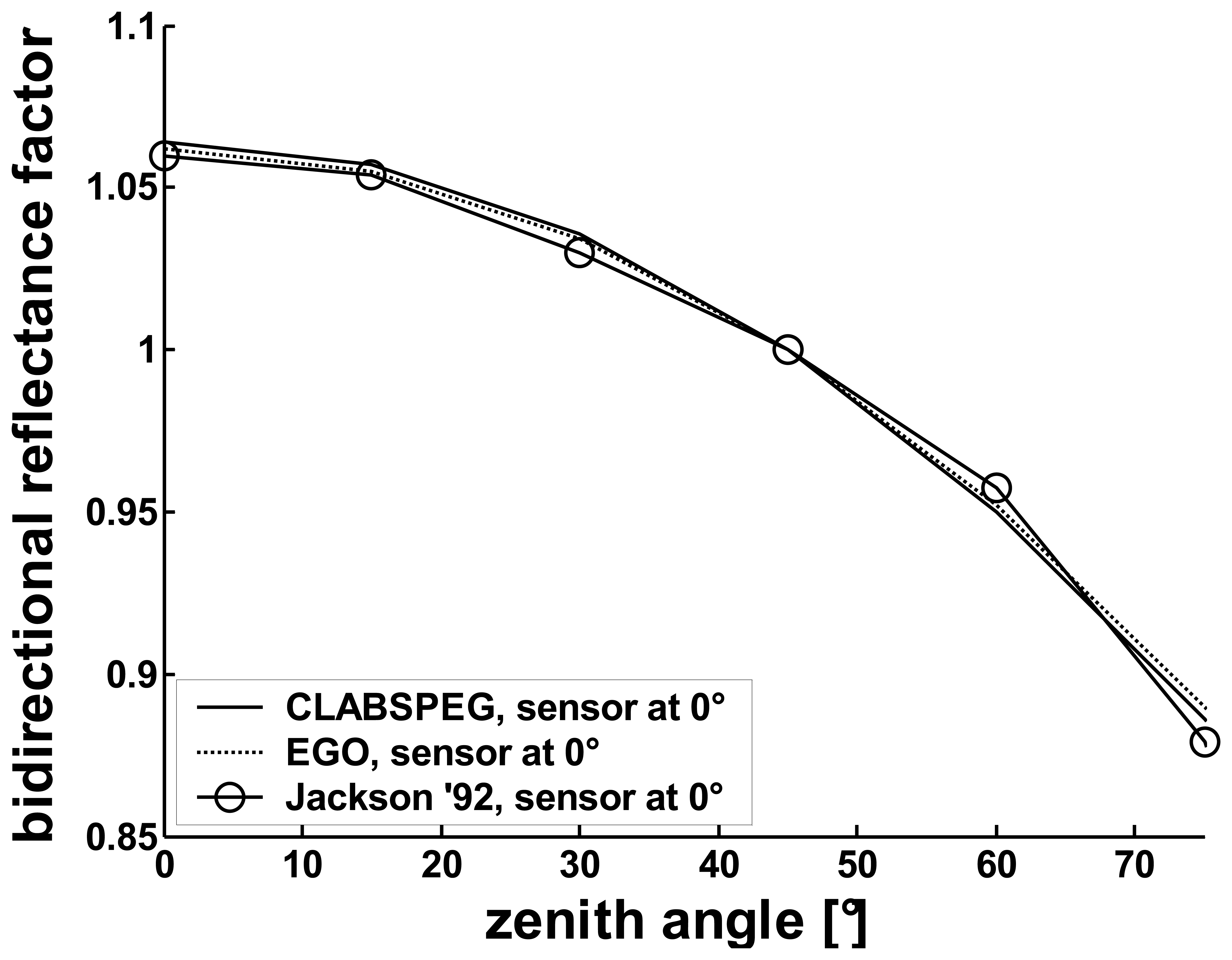
5.1.1. The Spectralon, as non-Lambertian body

The reflectance characteristics of the Spectralon panel were investigated concerning the deviation of the panel from a perfect Lambertian reflector. These reflectance characteristics are partly known from Labsphere's calibration procedure even though the albedo, ρ, which describes the wavelength dependent absorption of the Spectralon panel, derives from one specific measurement taken at 8° illumination angle. Furthermore, it should be noted that differences among Spectralon reference panels are sufficiently small [36] and preserve their anisotropy within 2% [37], while [17] used the Spectralon correction algorithms, covering the range of 450 nm to 1000 nm, provided by [28].
The hemispherical irradiance for the lamp at nadir position was used, determined with Equation (2), in order to correct the Spectralon's deviation from a perfect Lambertian body. The non-parallelism of the light source intensity was corrected by normalizing the irradiance intensities to the CLabSpeG center point [28].
According to equations (1) and (3), the panels Bidirectional Reflectance Factors Rref can therefore be determined by
R ref ( θ i , ϕ i ; 0 ; λ ) = L ref ( 0 ; θ r , ϕ r ; λ ) π E i ( 0 ; λ )
where Lref is the radiance reflected from the Spectralon reflectance panel and Ei the hemispherical irradiance for the lamp at nadir. A second-order polynomial function was used to interpolate the values of Rref among the different zenith positions of the light source. Appendix A presents the coefficients for calculating spectral Bidirectional Reflectance Factors Rref for the Spectralon panel in accordance with the calibration certificate provided by Labsphere for the 350 nm – 2500 nm wavelength range. The corresponding polynomial coefficients for Rref are applied to Eq. 4 to correct the nonideal reflectance characteristics of the Spectralon reference panel.
In figure 4, the polynomial functions are compared with the values extracted by [28] using as a comparison measure the standard deviation extracted from 11 calibrated Spectralon panels by [36]. All of the data are within one standard deviation of the measurements of [36], namely 0.0040 at 15° and 0.0076 at 75°.
Moreover, the percentage difference was extracted among the polynomial functions derived in our experiment and the functions of [28] for the wavelengths between 450 nm and 1000 nm and the maximum values are presented in table 3.
The differences in percentage indicate that the polynomial functions presented a similar behavior, exposing a stronger non-Lambertian behavior at higher wavelengths, with a maximum difference of 3.23% present at 75° source zenith angle at 1000 nm. These differences are assumed to be present due to the different spectroradiometers used between EGO (GER-3700) and CLabSpeG (ASD JR) and the fact that [28] extrapolated radiance values for zenith angles higher than 55°.

5.2. Correction of the biconical effect

Since the laboratory goniometer captures biconical reflectance, a correction for the conicity should also be applied. The correction of the biconical light source and sensor geometry consists of the inversion of a forward modeling where a known BRDF target (e.g Lambertian) is used to calculate the BRF (Rtrue), given the heterogeneity of the illuminated area, the conical illumination and viewing geometries for each and any given light source sensor angular combination. Consequently the measured BRF values of the Spectralon are divided point by point with the simulated values providing the error induced due to the conical nature of the light source and sensor geometry [31]. Considering all the angular combinations it was found that the conicality of the light induces a relative error starting at 0.004% and reaching a maximum deviation of the order of 4.71% at the 75° light source over 75° sensor position.

5.3 Leaves

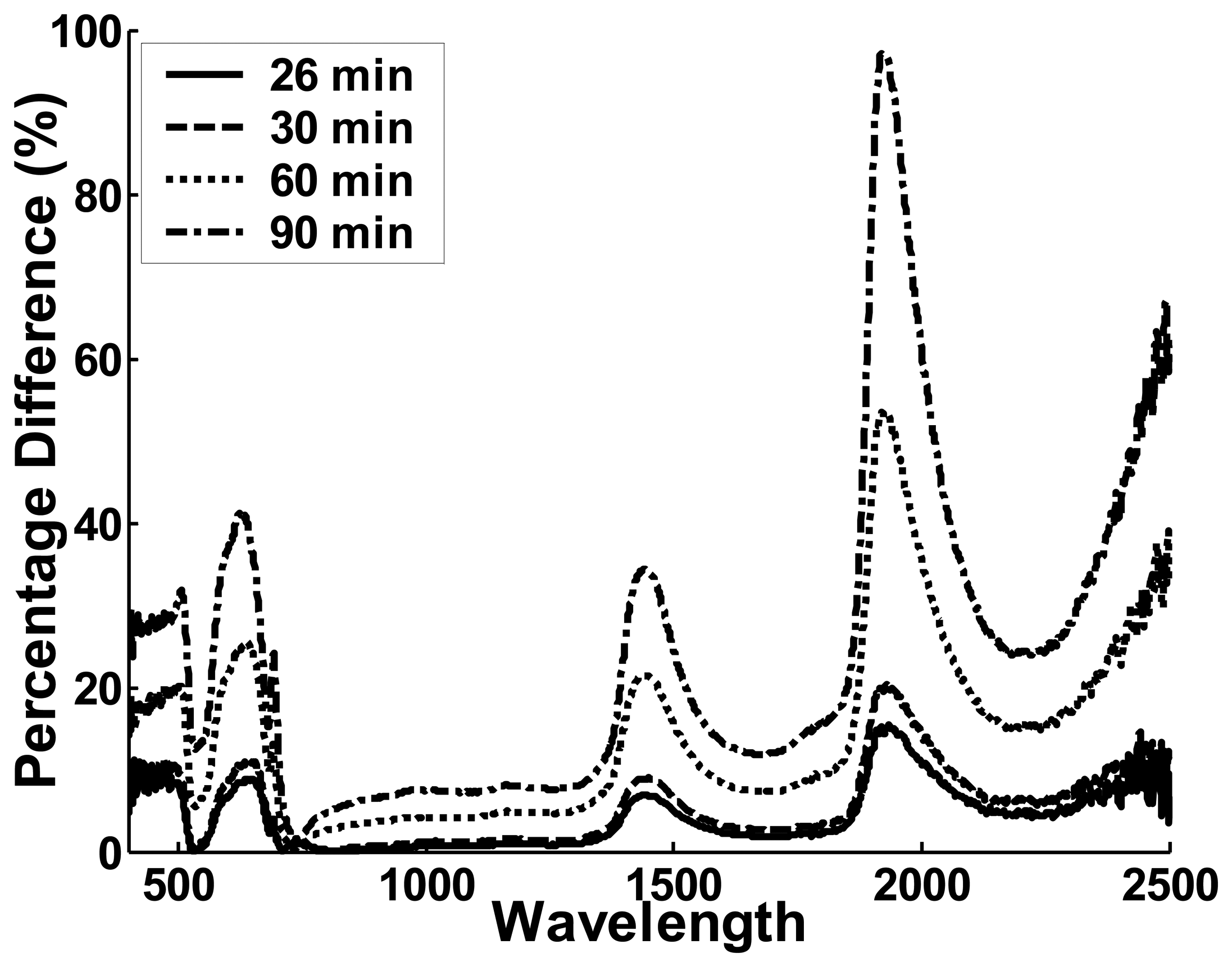
5.3.1 Leaf endurance under light source stress

A specific concern originating from the time needed to acquire BRF measurements is related to the duration a leaf has to spend on the sample plate and by extension under the light source. The reflectance behavior of a leaf under the light source conditions and the change in reflectance through time were evaluated before any BRF measurements were initiated. Hence, the reflectance from a leaf was periodically measured to gauge changes in reflection due to moisture loss, even though some researchers [25] assumed unchanged leaf optical properties for a period of less than an hour under their BRDF measurements. The change in reflectance of a leaf, from a static geometric position of light source (nadir) and sensor (60°) under the same laboratory conditions was measured every 5 minutes. By this the effect on leaf reflectance due to the light source heat is described, given a hemispherical BRF measurement cycle of 2.5 hours. As will be further indicated, this has specific implications related to sample spectral stability and durability.
The reflectance percentage difference (%) for all wavelengths, from the initial measurement was calculated and is presented for the first 26, 30, 60, and 90 minutes respectively in figure 5.
Considering the first 30 min of leaf endurance under the light source it was observed that the highest difference compared with a fresh leaf occurred in the water absorption bands of the infrared region with a peak at 1932 nm (20.29%) and at 1442 nm (8.93%), while the rest of the infrared part presented changes below 3%. In the visible domain it was noticed that as far as the green part is concerned (550 nm) the reflectance did not change and maintained the same values with a percentage difference of maximum 1.15%. The peak in reflectance change however occurred, in the visible region, at 641 nm with a difference of 11.21% after a period of 30 minutes. As the heat stress continued, the reflectance at certain wavelengths (660 nm, 1940 nm), changed rapidly while other spectral regions did not exhibit much of a reflectance difference even after a period of 2.5 hours (e.g., 850 nm).
Knowledge on these reflectance changes is important to determine the behavioral stability of the leaf sample during BRF measurements. In conclusion a full hemisphere BRF measurement of a single leaf is not feasible because of the long duration of the measurement cycle. We therefore, focused on selective BRF measurements of leaves instead. With a duration of less than 26 minutes, 12 BRF cycles were acquired for each light source zenith position covering all azimuth light source positions. Consequently, one leaf was used to measure the BRF for all light azimuth positions when the light source was at nadir, another for the light source at 15°, and so on. As far as the leaf size was concerned, the ASD sensor geometry and the associated field-of-view on the sample holder indicated that the sensing area exceeded the size of an average leaf at high zenith angles (75°). As a result the measurements at this “sun – sensor” zenith angle were excluded from the analysis. Consequently, complete leaf reflectance coverage at all possible light – sensor angle combinations are only reliable up to 60° sensor zenith.

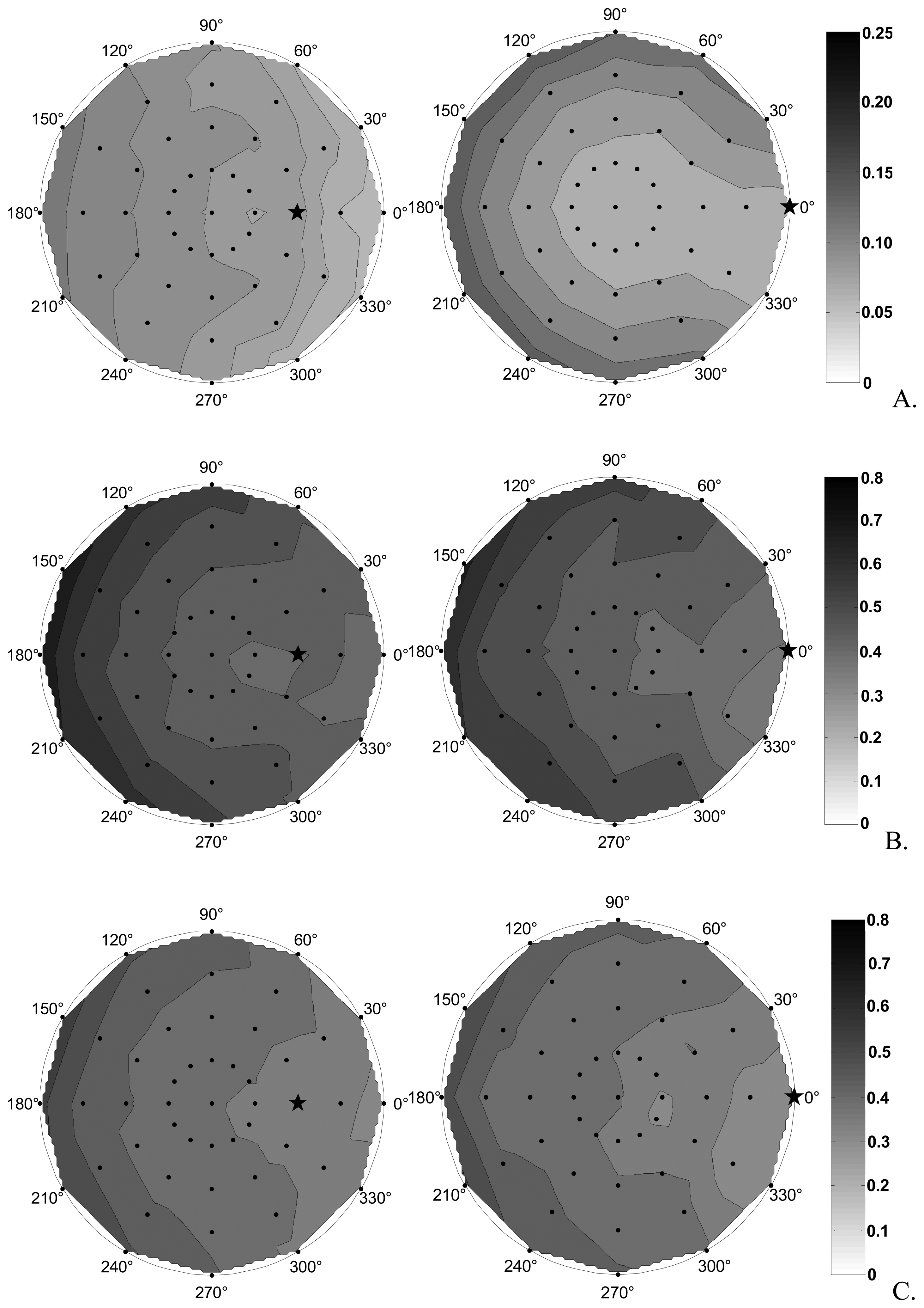
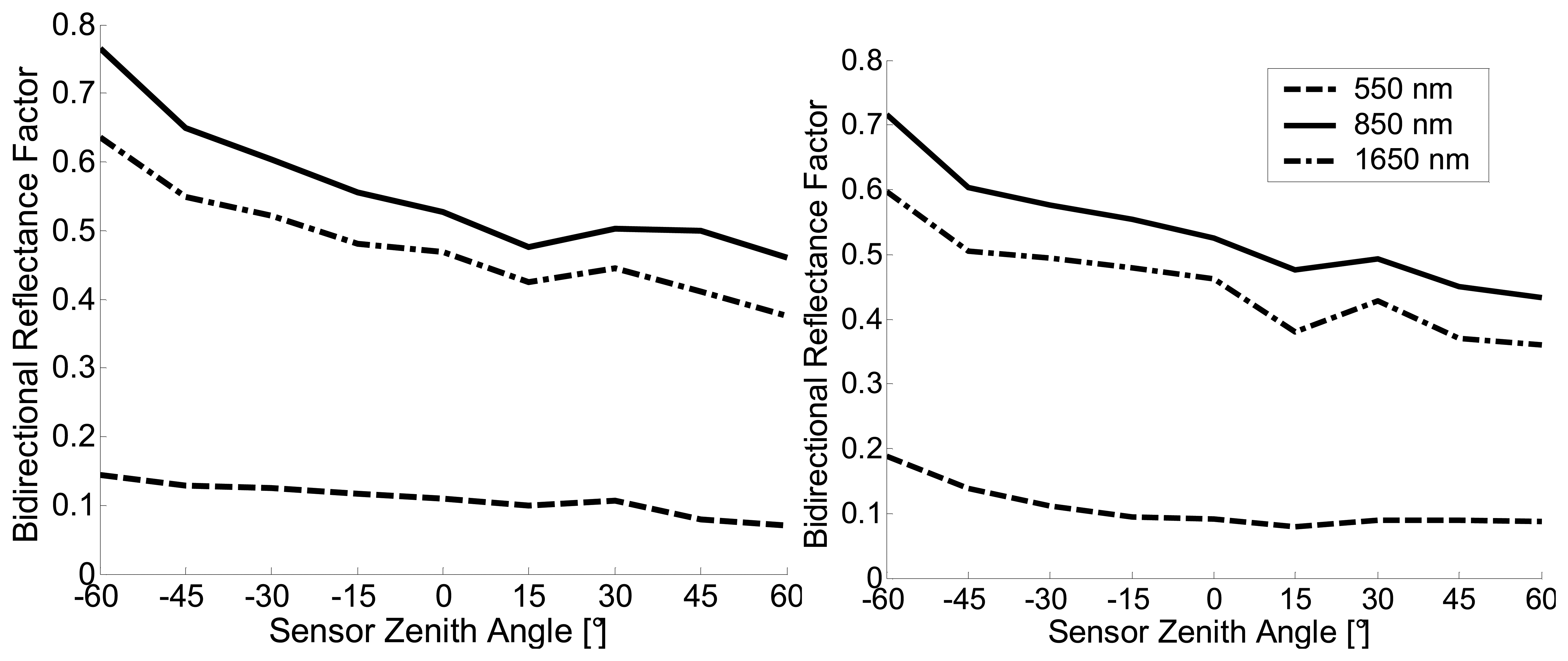
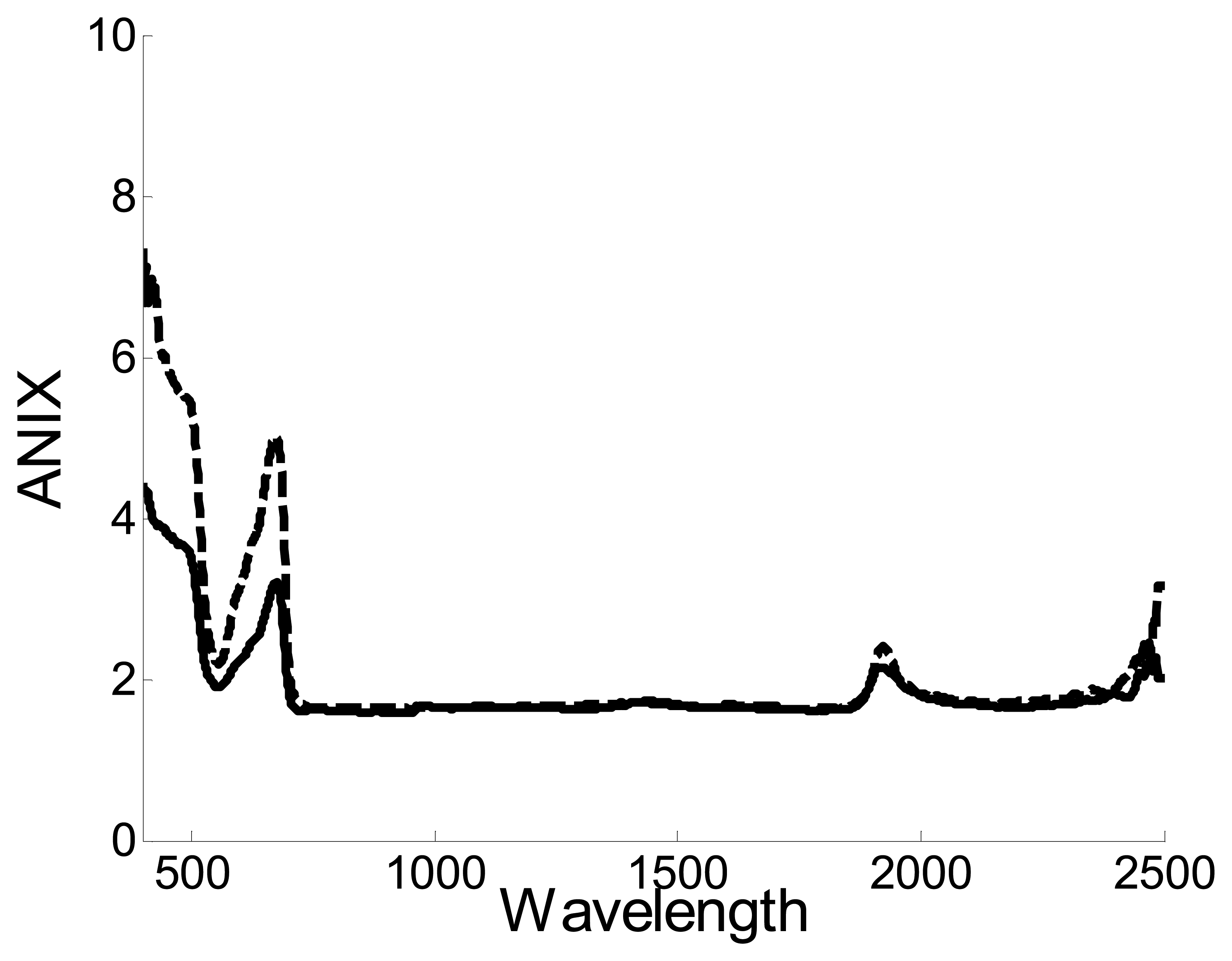
5.3.2 Leaf BRF acquisition

In August 2006, branches of two Fagus sylvatica L. trees were cut every morning from a forest stand near the gonio-reflectometer facilities and kept inside water for the period of the measurement cycle. This methodology resulted in preserving a branch in water for a maximum of 2 hours and a negligible time-span between the actual cutting of a leaf and the initiation of BRF measurements. 12 leaves were measured for each zenith position of the light source, resulting in a total of 60 leaves. All leaves were placed on the sample holder pressed between two metal frames, bearing a hole in the middle, to remain horizontally flat. The sample holder, as well as the upper surface of the metal frame was covered with a completely absorptive black textile (oscuratinto colour 211) that presents zero reflectance in the full dynamic range of the spectroradiometer so as to ensure that no reflectance is contributing from underneath and the surroundings of the leaf. Hence, transmitted light was extinct. Leaves were placed with the adaxial side facing upwards, with the main axis orientation towards the 0° of the light source azimuth and the 90° of the sensor.
The division of the two radiance cycles (leaf vs Spectralon) together with the Spectralon and conicality correction factors provided the reflectance of the leaf sample at each light - sensor angle combination. This results in a target reflectance for each such combination. Given that the amount of wavelengths collected (2151) prohibits a thorough analysis in the current paper and that our initial goal was to present the capabilities of the CLabSpeG spectrogoniometer, three wavelengths were chosen to represent the BRF behavior of a Fagus sylvatica L. leaf. These were located in the visible (550 nm), infrared (850 nm) and mid-infrared (1650 nm) regions. In figure 6 two angle combinations are presented with the light source at 0° azimuth and the zenith in 30° and 60° respectively.
The visualization of the Bidirectional Reflectance Factor of the Fagus sylvatica L. leaf shows, at 550 nm wavelength, a forward scattering at 30° zenith light source, ranging between 0.072 and 0.139 with a standard deviation of 0.012 while at an increased illumination zenith angle of 60° a profound reflectance value is exhibited in the principal plane at the specular angle, reaching a peak of 0.181 and a minimum of 0.08, with a standard deviation of 0.028. However, the reflectance differences at 850 nm and 1650 nm are less significant and follow a closer to a Lambertian shape for both light source zenith values. At both wavelengths maximum reflectance is obtained in the forward scattering plane while the minimum values are observed in the backscatter direction. At 850 nm we obtained reflectance values ranging from 0.74 to 0.46 for light source at 30° and 0.715 to 0.435 for light source at 60°, with a standard deviation of 0.055 and 0.06 respectively. Similar deviation but lower values are obtained for the reflectance measurements at 1650 nm. In figure 7 we present the principal plane of the above results highlighting the forward scattering present in our measurements.
These results are also confirmed by examining the degree of anisotropy of the distribution of the BRF via the anisotropy index (ANIX), presented for all wavelengths in figure 8. ANIX is the ratio of the maximum and minimum Bidirectional Reflectance Factors for a specific wavelength [38].
ANIX ( λ ) = ρ max ( λ ) ρ min ( λ )
It is noticed that ANIX factors portray similar values for all the wavelengths further the red edge region, while major differences are present in the visible part of the electromagnetic spectrum. Maximum values of 4.42 and 7.35 for 30° and 60°, respectively are extracted at 400 nm, while the minimum values are 1.57 at 944 nm for the 30° light position, and 1.62 at 963 nm for 60°. The minimum difference among the two angle configurations is present at 1022 nm with a value of 0.22, while maximum ANIX difference is 2.95 at 422 nm. Concluding, in table 4, we would like to provide the minimum and maximum relative standard deviation in percentage among the 12 leaves measured for each BRF angular combination and wavelengths mentioned above.

6. Discussion and Conclusion

The conducted calibration experiments with the new CLabSpeG instrument have demonstrated robust geometric accuracy, as well as sufficient radiometric stability and repeatability of the apparatus. CLabSpeG provides a unique capability for investigating the full BRDF of a material by supplying data in large array of light-sensor-zenith-azimuth hemispherical combinations. The high data acquisition speed makes CLabSpeG an ideal tool for capturing BRF of vegetative elements, such as leaves, given that their biochemical properties change over time mainly to leave water content loss effects. The apparatus is used for measuring BRF data of forest elements (e.g., leaves, bark, and soil). These materials are considered as non-isotropic and their reflectance is derived by rationing the measured target radiance with a previously measured radiance cycle of the Spectralon reference panel. An excellent use of CLabSpeG would be to assess BRDF data of thermally stable materials (e.g Spectralon, sand, wood) and potentially extract accurate albedo calculations. Thorough analysis was performed to provide accurate reflectance values, while correcting for the conical effect of the light source and providing an analytical reflectance correction factor matrix for the non-Lambertian reflection properties of the reference panel covering the electromagnetic wavelength for the range between 350 nm and 2500 nm. To our knowledge there exists no earlier published work on correction factors for wavelengths larger than 1000 nm. We consider essential that any attempt to measure reflectance of sensitive to heat materials in laboratory conditions should include a prior analysis of the impact of the light source on the material itself, since different wavelengths exhibit dissimilar behavior in reflectance under heat stress [39]. Furthermore it should be noted that bidirectional transmittance data would have been desirable to be able to obtain. However recent publications have established the hypothesis that transmittance of leaves is more isotropic than reflectance and presents a closer to Lambertian behavior [25-26].
Then, an attempt was made to demonstrate and quantify the non-Lambertian properties of Fagus sylvatica L. leaves by measuring the Bidirectional Reflectance Factor. A protocol of measuring leaf reflectance behavior was established and issues related to the nature of vegetative material, such as leaf reflectance variability among different wavelengths and the effect of drying on reflectance were investigated. Moreover it was showed that different wavelengths show different BRF patterns, while the Anisotropy Index for two angular configurations have shown that in the infrared the BRF variation is smaller than in the visible domain. The results of our observations were in agreement with previous published work in terms of the specular nature of leaf reflectance [21, 25] and in terms of the specular peak not being always restrained in the principal plane [20, 26]. Future analysis will focus on presenting different wavelength-dependent reflectance attributes, presenting the variability among azimuth and zenith light–sensor angle combinations. Parallel statistical analysis of all measured leaves will give an insight in the BRDF tendency of the Fagus sylvatica L. A better understanding of this variability furthermore could result in a reduction of the required number of measurements and thus the total acquisition time. The apparatus and the measurements derived from it can be applied in canopy reflectance models as validated input BRDF values. Laboratory measured BRDF data can be used along with ancillary structural information, to design and validate physically-based reflectance models while they can enhance the use of remote sensing data by extrapolating values for more than one aerial-satellite view angle, and define preferable viewing angles (satellite orbits) for specific applications and future missions.
Finally, CLabSpeG measurements could contribute to the computer graphics domain in generating a realistic representation of a forest stand ranging from satellite view up to close up zoom scale, even in the infrared region, when combined with transmittance data and accurate canopy architectural data [40]. It is recommended that future work focuses on classifying leaves of a number of species, based on age, type, and position in the tree. Such a classification likely will provide an insight to the reflectance homogeneity of leaf types and groupings within BRDF behavior of different species and most importantly create a basis for a future species specific BRDF library.

Acknowledgments

We would like to thank Dr. B. Hosgood and Dr. B. Pinty of the EGO at Ispra, Italy, Dr. M. Schaepman of the Wageningen University, The Netherlands, for helpful discussions about gonioreflectometer construction and calibration issues. We also like to thank L. Bousquet from the Institut de Physique du Globe de Paris, France, for his BRF graphical representation code. We also acknowledge the work performed by the anonymous referees and the journal editor for his useful comments and suggestions. Finally we thank CIT Engineering Geel, Belgium, for the mechanical construction of the device.

Appendix A.

Appendix A. Second-order polynomial coefficients for calculating spectral Bidirectional Reflectance Factors, Rref, for the Spectralon reflectance panel, used to correct the non ideal reflectance characteristics. Rref of a panel nadir measurement under an arbitrary source zenith angle θ can be calculated by Rref = a0 + a1 θ + a2 θ2. The differences between measured data and calculated values are referenced as relative root mean square errors in percentage (RMSE).
λ (nm)Coeff. α0Coeff. α1Coeff. α2RMSE (%)
3501.074-1.5904e-007-2.275e-0051.0821
4001.066-1.4206e-007-3.374e-0051.0824
4501.066-1.4290e-007-3.280e-0051.0819
5001.065-1.4382e-007-3.245e-0051.0820
5501.064-1.4460e-007-3.191e-0051.0818
6001.064-1.4506e-007-3.169e-0051.0818
6501.063-1.4572e-007-3.135e-0051.0818
7001.064-1.4612e-007-3.115e-0051.0818
7501.064-1.4658e-007-3.089e-0051.0818
8001.061-1.4668e-007-3.058e-0051.0816
8501.058-1.4662e-007-3.053e-0051.0815
9001.062-1.4664e-007-3.066e-0051.0816
9501.061-1.4782e-007-3.000e-0051.0816
10001.063-1.4098e-007-2.877e-0051.0780
10501.064-1.4174e-007-2.826e-0051.0779
11001.060-1.4080e-007-2.852e-0051.0778
11501.059-1.4130e-007-2.800e-0051.0776
12001.064-1.4184e-007-2.812e-0051.0778
12501.058-1.4096e-007-2.821e-0051.0776
13001.050-1.4050e-007-2.745e-0051.0768
13501.061-1.4148e-007-2.803e-0051.0776
14001.048-1.3984e-007-2.781e-0051.0769
14501.041-1.3966e-007-2.733e-0051.0764
15001.043-1.4032e-007-2.704e-0051.0764
15501.052-1.4142e-007-2.735e-0051.0771
16001.054-1.4142e-007-2.772e-0051.0774
16501.059-1.4224e-007-2.791e-0051.0778
17001.064-1.4360e-007-2.775e-0051.0782
17501.064-1.4358e-007-2.778e-0051.0782
18001.064-1.5060e-007-2.829e-0051.0811
18501.072-1.5006e-007-2.947e-0051.0819
19001.073-1.5086e-007-2.936e-0051.0821
19501.073-1.5116e-007-2.889e-0051.0818
20001.078-1.5198e-007-2.899e-0051.0822
20501.090-1.5324e-007-2.941e-0051.0829
21001.098-1.5436e-007-2.981e-0051.0837
21501.106-1.5582e-007-2.947e-0051.0839
22001.089-1.5224e-007-2.994e-0051.0830
22501.087-1.5258e-007-2.950e-0051.0827
23001.098-1.5460e-007-2.920e-0051.0832
23501.110-1.5624e-007-2.933e-0051.0840
24001.116-1.5304e-007-3.266e-0051.0855
24501.115-1.5862e-007-2.904e-0051.0847
25001.105-1.5832e-007-2.804e-0051.0840

References

  1. Privette, J.L.; Deering, D.W.; Wickland, D.E. Report on the workshop on Multiangular Remote Sensing for Env. App. NASA Technical Memorandum 113202 1997, 60. [Google Scholar]
  2. Nicodemus, F.E.; Richmond, J.C.; Hsia, J.J.; Ginsberg, I.W.; Limperis, T. Geometrical Considerations and Nomenclature for Reflectance, NBS Monograph; National Bureau of Standards, US Department of Commerce: Washington, D.C., 1977; p. 160. [Google Scholar]
  3. Li, X.; Strahler, A.H. Geometrical - Optical Modelling of a Conifer Forest Canopy. IEEE Trans. Geosci. Remote Sens. 1985, 23(5), 705–721. [Google Scholar]
  4. Jacquemoud, S.; Baret, F. PROSPECT: A Model of Leaf Optical Properties Spectra. Remote Sens. Environ. 1990, 34, 75–91. [Google Scholar]
  5. Qi, J.; Cabot, F.; Moran, M.S.; Dedieu, G. Biophysical Parameter Estimation Using multidirectional Spectral Measurements. Remote Sens. Environ. 1995, 54, 71–83. [Google Scholar]
  6. Pinty, B.; Verstraete, M.M.; Gobron, N. The effect of soil anisotropy on the radiance field emerging from vegetation canopies. Geophysical Res. Ltrs. 1998, 25(6), 797–800. [Google Scholar]
  7. Baranoski, G.V.G.; Rokne, J.G. Light Interaction with Plants, A Computer Graphics Percpective. Horwood Publishing 2004, 186. [Google Scholar]
  8. Wang, L.; Wang, W.; Dorsey, J.; Yang, X.; Guo, B.; Shum, H-Y. Real-time rendering of plant leaves. ACM Transactions on Graphics 1992, 26(2), 712–719. [Google Scholar]
  9. Phong, B-T. Illumination for computer generated pictures. Communications of the ACM 1975, 18(6), 311–317. [Google Scholar]
  10. Cook, R.L.; Torrance, K.E. A reflectance model for computer graphics. Richards, W., Ullman, S., Eds.; In Image Understanding; Norwood, NJ; Ablex, 1987; pp. 1–19. [Google Scholar]
  11. Lafortune, E.P.F.; Willems, Y.D. A theoretical framework for physically based rendering. Computer Graphics Forum 1994, 13(2), 97–107. [Google Scholar]
  12. Oren, M.; Nayar, K.S. Generalisation of lambert's reflectance model. Procceedings of SIGGRAPH'94. Computer Graphics Proceedings; Glassner, A., Ed.; 1994; pp. 239–246. [Google Scholar]
  13. Deering, D.W. Field measurements of bidirectional reflectance. In Theory and Applications of Optical Remote Sensing; Asrar, G., Ed.; Wiley: New York, 1989; pp. 14–65. [Google Scholar]
  14. Sandmeier, St.; Sandmeier, W.; Itten, K.I.; Schaepman, M.E.; Kellenberger, T.W. Acquisition of bidirectional reflectance data using the Swiss Field-Goniometer System (FIGOS). Proceedings of EARSeL symposium, Basel, Switzerland, Balkema, Rotterdam; 1995; pp. 55–61. [Google Scholar]
  15. Painter, T.H.; Paden, B.; Dozier, J. Automated spectro-goniometer: A spherical robot for the field measurement of the directional reflectance of snow. Rev. of Scient. Instr. 2003, 74(12), 5179–5188. [Google Scholar]
  16. Peltoniemi, I.J.; Kaasalainen, S.; Näränen, J.; Rautiainen, M.; Stenberg, P.; Smolander, H.; Smolander, S.; Voipio, P. BRDF measurement of understory vegetation in pine forests: dwarf shrubs, lichen and moss. Remote Sens. Environ. 2005, 94, 343–354. [Google Scholar]
  17. Bourgeois, C.S.; Ohmura, A.; Schroff, K.; Frei, H-J.; Calanca, P. IAC ETH Goniospectrometer: A Tool for Hyperspectral HDRF Measurements. Journal of Atmospheric and Oceanic Techn. 2006, 23, 573–584. [Google Scholar]
  18. Breece, H.T.; Holmes, R.A. Bidirectional scattering characteristics of healthy green soybean and corn leaves in vivo. Applied Opt. 1971, 10, 119–127. [Google Scholar]
  19. Kriebel, K.T. Measured spectral bidirectional reflectance properties of vegetated surfaces. Applied Opt. 1978, 253–259. [Google Scholar]
  20. Brakke, T.W.; Smith, J.A.; Harnden, J. Bidirectional Scattering of Light from Tree Leaves. Remote Sens. Environ. 1989, 29, 175–183. [Google Scholar]
  21. Walter-Shea, E.A.; Norman, J.M.; Blad, B.L. Leaf Bidirectional Reflectance and Transmittance in Corn and Soybean. Remote Sens. Environ. 1989, 29, 161–174. [Google Scholar]
  22. Koechler, C.; Hosgood, B.; Andreoli, G.; Schmuck, G.; Verdebout, J.; Pegoraro, A.; Hill, J.; Mehl, W.; Roberts, D.; Smith, M. The European Optical Goniometer Facility: Technical Description and First Experiments on Spectral Unmixing. Proceedings of IGARSS'94, Pasadena, 8-12 August, 1994; pp. 2375–2377.
  23. Serrot, G.; Bodilis, M.; Briottet, X.; Cosnefroy, H. Presentation of a new BRDF measurement device. The European Symposium on Remote Sensing, SPIE, Euporto, Barcelona, Spain; 1998; 3493, pp. 34–40. [Google Scholar]
  24. Schaepman, M.E.; Dangel, S. Solid laboratory calibration of a nonimaging spectroradiometer. Applied Opt. 2000, 39(21), 3753–3765. [Google Scholar]
  25. Bousquet, L.; Lachérade, S.; Jacquemoud, S.; Moya, I. Leaf BRDF measurements and model for speculalar and diffuse components differentiation. Remote Sens. Environ. 2005, 98, 201–211. [Google Scholar]
  26. Combes, D.; Bousquet, L.; Jacquemoud, S.; Sinoquet, H.; Varlet-Grancher, C.; Moya, I. A new spectrogoniophotometer to measure leaf spectral and directional optical properties. Remote Sens. Environ. 2007. [Google Scholar] [CrossRef]
  27. Schönermark, M.; Geiger, B.; Röser, H.P. Reflection Properties of Vegetation and Soil with a BRDF Data base; Wissenschaft und Technik Verlag: Berlin, 2004; p. 352. [Google Scholar]
  28. Sandmeier, St.; Muller, Ch.; Hosgood, B.; Andreoli, G. Sensitivity Analysis and quality Assessment of Laboratory BRDF Data. Remote Sens. Environ. 1998, 64, 176–191. [Google Scholar]
  29. Martonchick, J.V.; Bruegge, C.J.; Strahler, A.H. A Review of Reflectance Nomenclature Used in Remote Sensing. Remote Sensing Rev. 2000, 19, 9–20. [Google Scholar]
  30. Schaepman-Strub, G.; Schaepman, M.E.; Painter, T.H.; Dangel, S.; Martonchik, J.V. Reflectance quantities in optical remote sensing – definitions and case studies. Remote Sens. Environ. 2006, 103, 27–42. [Google Scholar]
  31. Dangel, S.; Verstraete, M.M.; Schopfer, J.; Kneubühler, M.; Schaepman, M.; Itten, K.I. Toward a Direct Comparison of Field and Laboratory Goniometer Measurements. IEEE Trans. Geosci. Remote Sens. 2005, 43(11), 2666–2675. [Google Scholar]
  32. Sandmeier, St. Acquisition of Bidirectional Reflectance Factor Data with Field Goniometers. Remote Sens. Environ. 2000, 73, 257–269. [Google Scholar]
  33. Analytical Spectral Devices, Inc. (ASD) Technical guide., 3rd ed.; 1999; p. 136. [Google Scholar]
  34. Solheim, I.; Hosgood, B.; Andreoli, G.; Piironen, J. Calibration and Characterization of Data from the European Goniometer Facility (EGO). Joint Research Centre Report EUR 17268 EN. 1996, 169. [Google Scholar]
  35. Sandmeier, S.R.; Itten, K.I. A Field Goniometer System (FIGOS) for Acquisition of Hyperspectral BRDF Data. IEEE Trans. Geosci. Remote Sens. 1999, 37(2), 978–986. [Google Scholar]
  36. Jackson, R.D.; Clarke, T.R.; Moran, M.S. Bidirectional Calibration Results for 11 Spectralon and 16 BaSO4 Reference Reflectance Panels. Remote Sens. Environ. 1992, 40, 231–239. [Google Scholar]
  37. Bruegge, C.; Chrien, N.; Haner, D. A Spectralon BRF data base for MISR calibration applications. Remote Sens. Environ. 2001, 76, 354–366. [Google Scholar]
  38. Sandmeier, St.; Muller, Ch.; Hosgood, B.; Andreoli, G. Physical mechanisms in hyperspectral BRDF data of grass and watercress. Remote Sens. Environ. 1998, 66, 222–233. [Google Scholar]
  39. Schaepman, M.E. Imaging Spectroscopy in Ecology and the Carbon Cycle: Heading Towards New Frontiers. Proceedings of the EARSeL 4th workshop on Imaging Spectroscopy, Warsaw, Poland; 2005; pp. 13–37. [Google Scholar]
  40. Gilabert, M.A.; Garcia-Haro, F.J.; Melia, J. A mixture modelling approach to estimate vegetation parameters for heterogeneous canopies in remote sensing. Remote Sens. Environ. 2000, 72, 328–345. [Google Scholar]
Figure 1. Picture and mechanical system setup of the Compact Laboratory Spectro-Goniometer (CLabSpeG). In the horizontal plane an aluminum rail (a) supports the light source arm (b) and rotates anti-clock wise with a resolution of 30°. A stationary arm (c) supports the hyperspectral sensor. Light source (f) and spectroradiometer (e) have an operational resolution of 15°. In the centre there is the sample holder including a leaf (d), rotating clock-wise with a resolution of 30°.
Sensors 07 01846f1
Figure 2. The changing footprint area of the sensor's field of view for various zenith angle positions. The dimensions are calculated for a 1° field-of-view and a distance of 0.35 m between the sensor and the surface.
Sensors 07 01846f2
Figure 3. Changing radiance intensity of light source footprint. Light was at 15° zenith and 90° azimuth. Radiance was measured over the Spectralon at 600 nm. The six grid values correspond to the viewing area for various sensor zenith angle positions while in 0° azimuth. Maximum intensity occurs at nadir position of the sensor, while minimum intensity value corresponds to 75°. In between values corresponds to 15° increment. Values were normalized to nadir intensity and presented on the graph.
Sensors 07 01846f3
Figure 4. Bidirectional Reflectance Factors of the Spectralon for 3 different settings: 1) CLabSpeG Spectralon panel with θr = 0° at 650 nm; 2) EGO Spectralon panel at 650 nm measured by [28] with θr = 0°; and 3) average of 11 Spectralon panels at 655 nm measured by [36] with θr = 0°. The differences among the three polynomial equations presenting the Bidirectional Reflectance Factors are smaller than the standard deviation (0.0040 at 15° and 0.0076 at 75°) found by [36] among the 11 Spectralon panels.
Sensors 07 01846f4
Figure 5. Percentage differences along the electromagnetic spectrum region of 400–2500 nm for a Fagus sylvatica L. leaf under a tungsten halogen lamp for a period of 26, 30, 60, and 90 minutes. Changes in the reflectance values are detected with profound differences in the water absorption bands.
Sensors 07 01846f5
Figure 6. Bidirectional Reflectance Factor of a Fagus sylvatica L. leaf at 550 nm (A), 850 nm (B) and 1650 nm (C), for light source position set at 0° azimuth and 30° zenith (left) and at 0° azimuth and 60° zenith (right). The sensor is azimuthally positioned all over the hemisphere and ranges in zenith between 0° and 60°, with 15° increments. Sensor's positions are marked by dots, while incident direction is presented by a star. The bar scale indicate reflectance values.
Sensors 07 01846f6
Figure 7. Bidirectional Reflectance Factor of a Fagus sylvatica L. leaf in the principal plane for three wavelengths. Namely 550 nm, 850 nm and 1650 nm. The light source position is set at 0° azimuth and 30° zenith (left graph) and 0° azimuth and 60° zenith (right graph). The sensor is on the principal plane with minus zenith values corresponding to forward scattering. The legend is the same for both graphs.
Sensors 07 01846f7
Figure 8. Anisotropy Index (ANIX) factor (the ratio of the maximum and the minimum Bidirectional Reflectance Factor for a specific wavelength) for a Fagus sylvatica L. leaf is presented at all wavelengths between 400 nm and 2500 nm, for light source position set at 0° azimuth and 30° zenith (solid line) and at 0° azimuth and 60° zenith (dotted line).
Sensors 07 01846f8
Table 1. Mean Radiance differences and Standard Deviation in (%), relative to the centre of the light source for all light source azimuth positions (mean values) and for different light source zenith positions. Sensor readings were acquired for all zenith positions.
SENSOR Zenith
LIGHT SOURCE Zenith15°30°45°60°75°
15°3.94 ± 1.735.84 ± 4.853.79 ± 2.845.98 ± 5.065.44 ± 3.6311.64 ± 8.80
30°17.68 ± 3.4012.91 ± 5.8616.04 ± 7.2610.23 ± 5.0310.36 ± 5.8412.76 ± 8.31
45°37.84 ± 4.2833.59 ± 7.2034.83 ± 5.4527.56 ± 9.8827.40 ± 8.5218.57 ± 12.77
60°64.38 ± 2.9861.18 ± 4.9661.79 ± 4.0456.36 ± 5.8553.42 ± 7.3730.83 ± 20.50
75°83.25 ± 1.2182.04 ±1.8481.64 ± 1.4379.03 ± 2.5175.02 ± 4.1851.29 ± 25.52
Table 2. Combination of light source and sensor positions that present lower than expected reflectance values due to shadow-casting on the target. Major signal drop positions exist at 60° and 90° azimuth of the light source and are attributed to construction artifacts.
Light AzimuthLight (L) over sensor (S) Zenith positions
0°L/0°S
30°0°L/0°S
60°15°L/75°S, -15°L/60°S, 15°L/45°S, -15°L/30°S, -15°L/15°S, and 0°L/0°S
90°-75°L/75°S, -60°L/60°S, -45°L/45°S, -30°L/30°S, -15°L/15°S, and 0°L/0°S
120°15°L/60°S, -15°L/45°S, 15°L/30°S, -15°L/15°S, and 0°L/0°S
150°0°L/45°S, 0°L/30°S, 0°L/15°S, and 0°L/0°S
Table 3. Maximum percentage differences between second-order polynomial functions to calculate the Bidirectional Reflectance Factors Rref extracted with CLabSpeG and EGO goniometers. Light source is at nadir position and sensor at 75° zenith.
Wavelength (nm)4505005506006507007508008509009501000

Difference (%)1.691.440.950.750.510.210.531.061.541.391.923.23
Table 4. Minimum and maximum standard deviation in percentage among the 12 leaves measured for two BRF angular positions. Namely for the light source at 30° zenith and 0° azimuth and for the light source at 60° zenith and 0° azimuth. Values for three wavelengths are presented.
Wavelength (nm) and Light Source Zenith (°)

STD (%)550 (30°)550 (60°)850 (30°)850 (60°)1650 (30°)1650 (60°)
MIN5.392.93.874.212.783.75
MAX17.3817.7310.3610.118.309.49

