Value-at-Risk for South-East Asian Stock Markets: Stochastic Volatility vs. GARCH


1
John von Neumann Institute, Vietnam National University, Ho Chi Minh City, Vietnam
2
Queen’s Management School, Queen’s University Belfast, Belfast BT7 1NN, UK
3
Faculty of Business and Economics, Technische Universität Dresden, 01062 Dresden, Germany
4
Institute for Operations Research and Computational Finance, University of St. Gallen, 9000 St. Gallen, Switzerland
*
Author to whom correspondence should be addressed.
J. Risk Financial Manag. 2018, 11(2), 18; https://doi.org/10.3390/jrfm11020018
Submission received: 16 March 2018
/
Revised: 3 April 2018
/
Accepted: 3 April 2018
/
Published: 5 April 2018
(This article belongs to the Special Issue Trends in Emerging Markets Finance, Institutions and Money)
Abstract
:This study compares the performance of several methods to calculate the Value-at-Risk of the six main ASEAN stock markets. We use filtered historical simulations, GARCH models, and stochastic volatility models. The out-of-sample performance is analyzed by various backtesting procedures. We find that simpler models fail to produce sufficient Value-at-Risk forecasts, which appears to stem from several econometric properties of the return distributions. With stochastic volatility models, we obtain better Value-at-Risk forecasts compared to GARCH. The quality varies over forecasting horizons and across markets. This indicates that, despite a regional proximity and homogeneity of the markets, index volatilities are driven by different factors.
1. Introduction
The members of the Association of Southeast Asian Nations (ASEAN)1 already produce 3.43% of the worldwide Gross Domestic Product (GDP) in 2016 and even the economically smaller countries such as Vietnam are on the rise. The ASEAN-62 have an annual GDP growth from 2016 to 2017 of 4.91% and share 4.48% of the world’s average annual GDP growth of 3.6%.3
However, the crisis of Asian markets in 1997 shows that investors have to accept other risks than those in industrialized and developed western economies. The Asian crisis is characterized by an unparalleled contagion throughout the markets and extreme market and currency movements. While this crisis has almost only regional macroeconomic effects, consequences and lessons from it are drawn globally (Hunter et al. 1999). Another example for very high contagion in these markets are disruptions in the wake of the global financial crisis beginning in 2007, as Asian emerging markets do not offer diversification potential (Kenourgios and Dimitriou 2015).
During times of crises as well as during more moderate times of daily business, investors and portfolio managers face the challenge to properly estimate and model dispersion in market prices, formalized in its volatility or variance. Depending on the trading position, financial risk has to be determined for the long and short position. While the long trading position (e.g., having bought an asset to sell it at a later point) is concerned with falling prices or negative returns, the short trading position (e.g., short-selling an asset, i.e., borrow an asset and directly sell, to re-buy it at a later point to give it back to the owner) faces rising prices or positive returns (Giot and Laurent 2003). This is of particular importance if asymmetric distributions, such as the Skewed Student’s-t distribution, are found to provide a better resemblance of the empirical price return distribution than symmetric distributions like the Normal or Student’s-t distribution. In this work, we use the Value-at-Risk (VaR) as a measure for financial risk, which is determined by the volatility of an investment. Albeit the fact that VaR has been replaced by Expected Shortfall as the main tool to determine the minimum capital requirements for banks under the Basel framework, VaR is still in place for backtesting the internally used risk models (Basel Committee on Banking Supervision 2016). Here, we incorporate two competing classes of volatility models. Within the framework of Generalized Autoregressive Conditional Heteroskedasticity (GARCH) models (Bollerslev 1986; Engle 1982), we model volatility conditional on its past. This allows for including volatility clusters with periods of high and low market movements. In the next step, the Asymmetric Power ARCH (Ding et al. 1993) is applied to account to asymmetric news impact on volatility. Another so-called stylized fact is the long lasting dependence of shocks in a time series known as long memory. The Fractionally Integrated GARCH (FIGARCH, (Baillie et al. 1996)) model is able to depict this pattern. The Fractionally Integrated Asymmetric Power ARCH (FIAPARCH) of Tse (1998) combines both long memory and asymmetry. The second class of models is based on the stochastic volatility (SV) model introduced by Taylor (1986). In addition to the standard SV model, we implement specifications that are able to depict the leverage effect as well as heavy tails. We use both classes to forecast the volatility over specific horizons based on estimates of a training window. With these variance forecasts, we then predict the VaR. These VaR predictions are evaluated and compared over different markets against standard approaches such as the non-parametric Historical Simulation (HS).
In this work, we focus on six major ASEAN stock market indices. Given the regional proximity and general similarity of these markets, we aim to understand if this also yields comparable variance properties. This would imply that methods of modeling and forecasting volatility as well as the VaR have comparable performances across the markets and that these markets could be grouped. While there is a plethora of literature on variance modeling for commodities, stock markets, and exchange rates of developed countries, academic advances on Asian stock indices and their comparison is relatively sparse. Walther (2017) identifies a sufficient performance of GARCH with a symmetric Student’s-t distribution as well as FIAPARCH with a skewed Student’s-t distribution in terms of variance and VaR forecasting for Vietnamese stock indices. Brooks and Persand (2003) show that asymmetric approaches work well to forecast the VaR for the Singapore and Thailand equity indices. So and Yu (2006) use different GARCH models to estimate the VaR in twelve different stock markets including Indonesia, Malaysia, Thailand, and Singapore. Su and Knowles (2006) perform a VaR analysis of Mixture Normal models on stock indices including Malaysia, Singapore, and Thailand. Lastly, McMillan and Kambouroudis (2009) and Sharma and Vipul (2015) provide large studies of different equity indices (including many ASEAN countries) for VaR forecasting.
Our results suggest that the volatility structures in the ASEAN markets is heterogeneous and include various so-called stylized facts. Hence, we observe that more sophisticated models provide better forecasts than standard approaches. However, given the different dynamics in the markets, we cannot conclude with one explicit model choice over all ASEAN equity markets.
2. Methodology
2.1. Estimating Volatility
We incorporate two alternatives to calculate the daily volatility. The first model belongs to the family of Generalized Autoregressive Conditional Heteroskedasticity (GARCH) models originating from Engle (1982). Within the GARCH framework, the process for returns is formulated as
where denotes the mean, the conditional variance is defined as , and the random variable follows a Skewed Student’s-t distribution4 with i.i.d. for all (Hansen 1994). Here, is a sigma algebra containing all past information of returns and conditional volatilities up to time .
The distributional parameter for the Skewed Student’s-t distribution, the degrees-of-freedom and the skewness , are estimated along with the model parameters. For the conditional variance , we consider the GARCH(1,1) specification of Bollerslev (1986), which reads:
A well-known characteristic of volatility is the negative correlation with returns, also known as the leverage effect (Black 1976; Christie 1982). In order to cope with this stylized fact, we implement the Asymmetric Power ARCH (APARCH, (Ding et al. 1993)), which is defined as:
where refers to the leverage parameter indicating whether negative or positive shocks have a larger impact on the daily volatility. For example, an estimated reveals that negative residuals increase the conditional volatility more than their positive equivalents, which is of particular interest for shocks.
We include the Fractionally Integrated GARCH (FIGARCH, (Baillie et al. 1996)) to cover the long memory effect. The standard FIGARCH(1,d,1) reads:
where
with the long memory parameter d and the lag operator L. To combine the leverage and the long memory effect, Tse (1998) proposed the Fractionally Integrated APARCH (FIAPARCH):
Note that the ARCH(∞) representation in Equations (3) and (5) is carried out using the fast fractional differencing method of Klein and Walther (2017) with truncation lag 5000. All GARCH-type models introduced above are estimated with maximum-likelihood estimations (MLE), ensuring that non-negativity and stationarity conditions, if applicable, hold for each model. All parameter estimates and robust standard errors following Bollerslev and Wooldridge (1992) are available upon request.
As an alternative to the GARCH framework, we also consider the stochastic volatility framework. Stochastic volatility models belong to the family of state-space models (Sarkka 2013, ch. 4). The standard stochastic volatility (SV) model is introduced by Taylor (1986) as
The SV model contains two noise processes, and , respectively accounting for the return shocks and the volatility shocks. In the SV model above, and are independent.
Harvey and Shephard (1996) introduce a more general setting where the noise processes and are correlated as
instead of being independent as in Equation (8). The correlation coefficient accounts for the leverage effect, defined as the negative correlation between shocks on return and volatility (i.e., ). This model is called the asymmetric SV model or SV-leverage (SV-L) model.
We consider a third stochastic volatility model where the return shocks follow Student’s t-distribution with degrees of freedom. It allows more extreme observations than with Gaussian return shocks as the Student’s t-distribution has heavier tails. The volatility shocks follow the standard Gaussian distribution. In this model, and are independent. It is referred to as the SV-t model.
We end up with three different stochastic volatility models: the SV model (Gaussian and independent shocks), the SV-L model (Gaussian and correlated shocks), and the SV-t model (t-distributed return shock, Gaussian volatility shock, independent shocks). In the three models, the parameters are estimated by Bayesian inference using the Markov Chain Monte Carlo (MCMC) sampling algorithms from Chan and Grant (2016).5
Lastly, we consider the RiskMetrics approach, the historical simulation, as well as the semi-parametric filtered historical simulation, which we explain in detail in the next subsection.
2.2. Value-at-Risk Forecasting and Backtesting
One of the most important financial risk measures is the Value-at-Risk. The VaR is usually defined as a specific loss, which is not exceeded for a given probability (e.g., %).
When using GARCH models, the k-days ahead VaR forecast is simply derived by a k-steps forecast of the variance based on the estimated parameters at time T, , which is then applied in the general VaR calculation scheme, yielding
where is the estimated mean, is the estimated conditional variance, and and are the estimated distributional parameters from the training set . denotes the a quantile function of the Skewed Student’s-t distribution with degrees-of-freedom parameter and skewness . Note that we only forecast the variance. Hence, in the VaR forecast, the quantile function depends on the estimated insample parameters, which are not forecasted separately. The calculation of the forecasted variance depends on the specific GARCH model. In this sense, there exists a closed form solution for the GARCH(1,1) k-days ahead forecast while, for the APARCH, FIGARCH, and FIAPARCH, the forecasts are calculated iteratively.6
With stochastic volatility (SV, SV-L, SV-t) models, we approximate the conditional distribution of the returns at the forecast horizon given the observed returns non-parametrically, i.e., the conditional distribution of given . We use particle filtering, a sequential Monte Carlo algorithm for state-space models (Sarkka 2013, chp. 7). The particle filter approximates the conditional distribution of the volatility given the returns in the form of a sample of so-called “particles”. This sample is propagated k times according to the volatility dynamics (Equation (7)), which is the same in the three stochastic volatility models. Then, from the volatility sample at time , a return sample is generated according to the return model (Equation (6)). We compute the VaR by taking the empirical quantiles of this return sample.
For the RiskMetrics approach (Longerstaey and Spencer 1996)—also known as Exponentially Weighted Moving Average (EWMA)—we use the standard GARCH-like case with fixed parameters , , and for Equation (1). Since the RiskMetrics model is not stationary, we use the estimate for all k-days ahead forecasts.
Lastly, we derive VaR forecast non-parametrically by the Historical Simulation (HS) and the semi-parametric Filtered Historical Simulation (FHS). The former method takes the past 250 returns as possible scenarios of a future return distribution and the VaR is calculated from the empirical a-quantile of the past returns, i.e.,
For the FHS, we follow Barone-Adesi et al. (1999). The technique combines the aforementioned GARCH and HS. To calculate the VaR, we estimate the parameters for a GARCH model with Skewed Student’s-t innovations over the whole insample. From the parameters, we derive a k-days ahead volatility forecast. Moreover, we calculate the empirical a-quantile from the most recent 250 standardized and centered GARCH residuals. The volatility forecast is then multiplied with the empirical quantile to estimate the VaR:
where
is the standardized and centered GARCH residual.
To evaluate the quality of the VaR forecasts for the different models and classes, we use four different VaR tests: the regulatory traffic light test, the conditional coverage test, the multi-level unconditional coverage test, and the loss function based comparison. In what follows, we refer to VaR violations or exceptions for the cases, where for the long trading position and where for the short trading position.
The Basel traffic light backtest (Basel Committee on Banking Supervision 2016) sorts VaR test results in three different zones. The test uses the 1-day ahead VaR for the last 250 trading days. A model is considered in the green zone, if four or less VaR violations occurred in that period. The yellow zone includes models yielding between five and nine exceptions. Lastly, the red zone covers all models with more than nine violations. The idea behind this color scheme is that the yellow zone is a buffer area for models that violate the VaR too often due to “bad luck” (type I error). Thus, banks only have to adjust their calculated minimum capital requirements by a fixed factor. However, models in the red zone are not allowed to be used; instead, the standard approach of the Basel framework has to be employed. Here, we calculate the traffic light test on a rolling time frame over the whole out-of-sample period and report how many days each model appears in the green, the yellow, or the red zone, respectively. Doing so, we gain a regulatory perspective of the results of the VaR forecasts.
In order to account for possible clustering of VaR violations, we include the conditional coverage test proposed by Christoffersen (1998). The test combines the unconditional coverage test with a test for the independence of VaR exceptions. Independence is assumed if the VaR violations do not follow a first order Markov chain. Thus, the test procedure penalizes models not only for an undesirable amount of violations, but also for not adjusting quickly after an exception occurred. Unfortunately, the test only evaluates a certain quantile and not the whole tail of the distribution.
The multi-level coverage test of Pérignon and Smith (2008) resembles a joint unconditional coverage test for three VaR levels at , , and . Thus, the test is able to evaluate the whole tail in one single test. The test compares the actual coverage ratio (number of VaR violations to length of observation period) with the preferred one (i.e., the VaR level a) based on a likelihood ratio test. Hence, only the absolute number of VaR violations is important to that test and it penalizes too conservative models as well as too optimistic models. However, the test is not designed to cope with clustering of VaR violations.
The outcome of the two presented backtests can only decided whether a particular model pass the requirements of being in the admired VaR coverage zone and not having clustered violations. Nevertheless, the backtests cannot be used to compare the VaR forecasts among a given set of models. Therefore, we incorporate a loss function based comparison. Here, we follow the idea of Angelidis and Degiannakis (2007). The authors suggest a two-stage approach: (1) all models are tested with a backtest such as the conditional coverage test; and (2) for the models that pass this test, the following VaR loss function suggested by Lopez (1998) is used:
The results of the loss functions for each model are compared with the Superior Predictive Ability test by Hansen (2005). We deviate from this procedure by using the Model Confidence Set (MCS, (Hansen et al. 2011)) in place of the Superior Predictive Ability test. The MCS yields a set of models of equally predictive ability. Thus, this procedure allows us to directly compare those models that pass the first-stage backtests.
3. Data
For our analysis of the main ASEAN financial markets, we include six country stock market indices. We choose the Indonesian Jakarta Stock Exchange Composite Index (JCI), the Kuala Lumpur Stock Exchange (KLSE) of Malaysia, the Philippines Stock Exchange PSEI Index (PCOMP), the Stock Exchange of Thailand (SET), the Singapore Strait’s Time Index (STI), and the Vietnam Ho Chi Minh Stock Index (VNI). Hence, we exclude the smaller stock markets of Myanmar, Cambodia, Laos, and Brunei from our analysis. The data is retrieved from Bloomberg in USD denominations for the period from 1 July 2006 to 30 June 2017. The period is chosen such that we obtain an equal number of observations of around for all indices accounting for individual holidays. We note that the VNI has some zero volume trading days before our chosen period. We calculate the daily returns of the stock indices by logarithmic price differences. For the forecasting exercise, we use the in-sample data from 1 July 2006 to 30 June 2017. This leaves us with an out-of-sample period from 1 July 2006 to 30 June 2017 and six years of 1-, 5-, and 20-days ahead forecasts for each index.
Descriptive statistics, provided in Table 1, show evidence that the empirical distributions of the index returns are of leptokurtic shape, indicated by an increased excess kurtosis. The JCI has the highest kurtosis of while the VNI features the lowest at . Moreover, all return series are skewed to the left; the series’ distributions have large negative returns with a higher probability compared to their positive counterpart. In comparison to indices of developed countries and global benchmarks, the empirical moments are quite extreme for indices, in particular the kurtosis, suggesting less diversification effects within each index. This highlights the relatively high risks associated with investing in these markets. In addition to the non-normal appearance of moments, we test for autocorrelation in the return series. The Ljung–Box (LB) test and the ARCH test both reject the hypothesis of no autocorrelation in the returns. The Augmented Dickey-Fuller (ADF) test rejects the hypothesis of a unit root in the return series. Based on these results, we assume the underlying distribution for the GARCH framework as Skewed Student’s-t. This distribution choice over alternatives such as the Normal or symmetric Student’s-t distribution ensures that we cover heavy tails and skewness found in the series, which impacts the parameter estimation and forecasting exercise. The series are depicted in Figure 1.
4. Results and Discussion
In this section, we compare the VaR forecast results for the six ASEAN equity indices. Therefore, we first present the results for each index individually and compare the findings afterwards. For each model, we estimate 1-, 5-, and 20-days ahead predictions that correspond to forecasts a day, a week, and a month ahead. Note that we do not forecast the VaR for the whole period, but for a certain point in the future. The results are presented in Table 2, Table 3, Table 4, Table 5, Table 6 and Table 7.
We start our analysis with the results from the Indonesian JCI (Table 2). The traffic light test does not find any of the models to be in the red zone. Moreover, we see that the GARCH is only present in the green zone, i.e., it never has no more than four violations in the whole out-of-sample for the long and the short trading position. However, the GARCH model does not pass the conditional coverage test by Christoffersen (1998) or the multilevel Pérignon and Smith (2008) test at any forecast horizon. There are a number of models that are able to depict the VaR at all quantiles under consideration for the 1-day ahead forecast on the long trading position: FHS, FIGARCH, SV, and SV-L, but only FIGARCH also shows the same ability on the short trading position. Its loss functions are satisfactory, but FIGARCH only belongs to the best performing models at the 2.5% quantile. The generally good performance of this model hints toward an elevated shock persistence in volatility. Regarding higher forecast horizon, it is only HS, which depicts good performance for all horizons on both trading sides with respect to the multilevel coverage test. The fact that HS is not able to pass the conditional coverage test may indicate that the model tends to build clustered violations, which is not covered by the multilevel coverage test.
The second equity index we analyze is the Malaysian KLSE (Table 3). Here, three models fail the regulatory traffic light test. While RiskMetrics has several days in the red zone of the long trading position, the HS and FHS models are included in the red zone for the short trading positions. Moreover, we observe some asymmetric behavior. RiskMetrics also completely fails to meet the criteria from the coverage test for the long trading position. However, it passes all tests for the short trading position. Almost the same behavior is observed for FIGARCH, with only exception for the 2.5% VaR of the conditional coverage test of Christoffersen (1998). On the long trading position, APARCH archives good results especially for 1-day ahead predictions. This suggests that both asymmetric news impact and long memory are present in this market’s volatility, which is further underlined by the performance of FIAPARCH. All stochastic volatility models pass the multilevel coverage test for the long trading position.
Next, we compare the results from the Philippine PCOMP index (Table 4). No model appears in the red zone of the traffic light test and thus they could be used without being replaced by the regulator. Here, we find five complete failures of models regarding the two statistical coverage tests. Neither RiskMetrics for the long trading position, nor GARCH or any stochastic volatility specification for the short trading position pass any of the tests. In addition, the two asymmetric GARCH models seem to have problems with the specific dynamics of the PCOMP index. Both APARCH and FIAPARCH perform very poorly with only a few passed tests. Generally, our model set does not include a clear candidate to be preferred in terms of VaR prediction performance. However, the HS and the FHS deliver the most promising results with respect to the multilevel test and the corresponding loss function results.
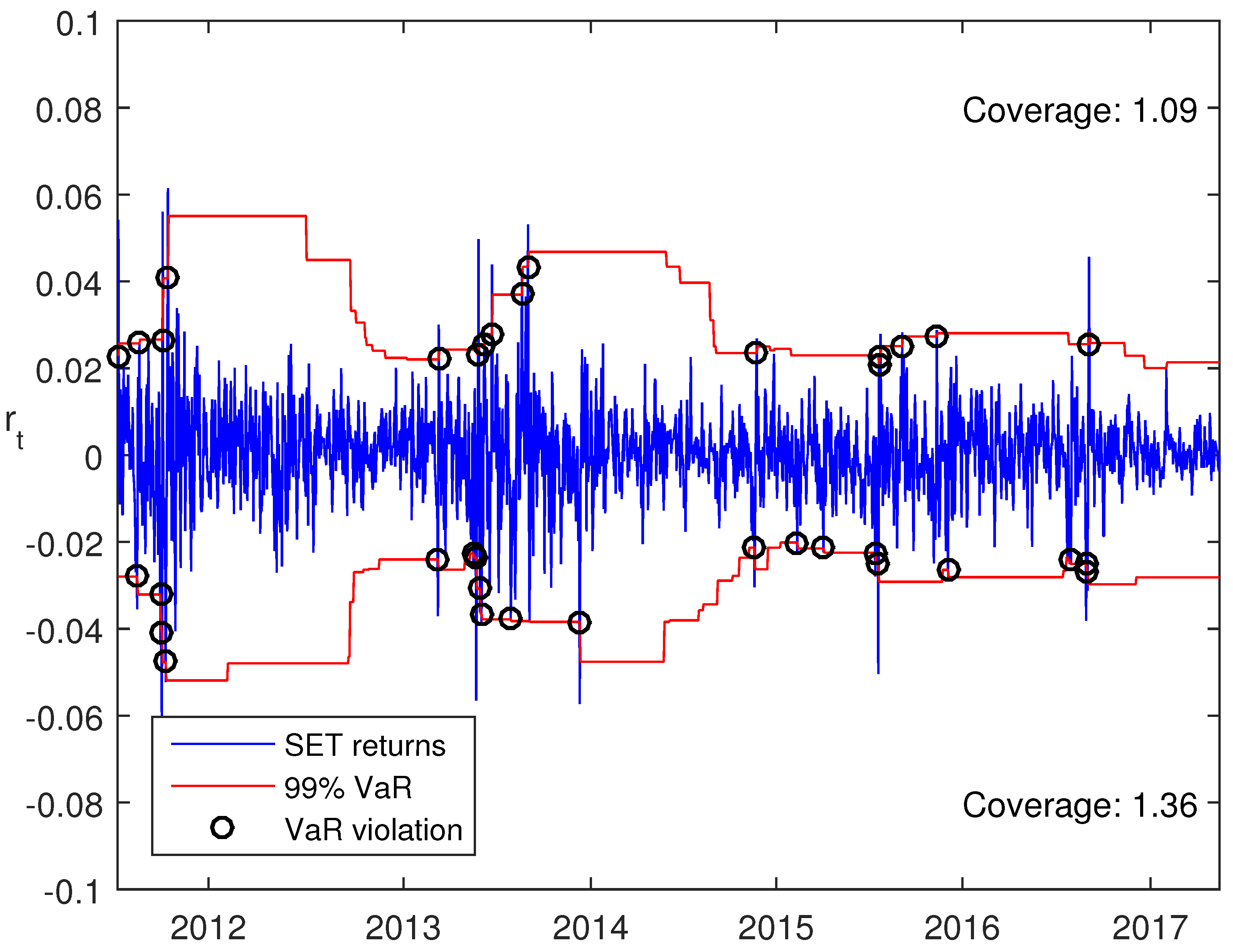
Table 5 presents the results from the VaR backtests for the SET, traded in Bangkok. From the traffic light test, it becomes apparent that RiskMetrics and FHS lead to several days in the red zone for the long trading position. The general result for SET is that most models can cope with the long trading position to some extend, but completely fail to depict the dynamics on the short trading position. The results from HS suggest that it can be used for 1-day ahead predictions for the long trading position. Even though it is not rejected by the unconditional coverage tests, it has problems to avoid clustering of the VaR violations. This behavior is illustrated in Figure 2. It shows the slow reaction to VaR violations on the short trading position and the overall good coverage for 1% VaR forecasts. Additionally, SV-t shows somewhat good performance on the long trading position, which is reflected in the fact that it passes all multilevel tests and belongs to the set of the best models for 5- and 20-days ahead. For both trading positions however, only FIAPARCH and HS have good results with respect to the multilevel test at least. Hence, we conclude that both asymmetry and long memory play an important role in the variance dynamics of SET, indicating that variance shocks have an extended persistence which is of asymmetric shape, however.
The STI from Singapore provides interesting results. From Table 6, we find that RiskMetrics (long) and FHS (short) are included in the red zone of the Basel traffic light test. Consequently, the models would be replaced by the regulatory standard approach and the institution would be penalized with a higher factor on the minimum capital requirements accounting for the bad model choice. Interestingly, RiskMetrics shows a good performance on the short trading side, where it passes most of the tests. The worst results are achieved by the GARCH model, which fails all tests, even though it stays in the green zone over the whole out-of-sample period. The stochastic volatility models show good performance on the long trading position but cannot provide equally good results on the short trading position. APARCH provides very good results for both trading positions regarding 1-day ahead forecasts, which indicates that asymmetries play an important role in the STI return structure.
Lastly, we compare the forecasting results for the Vietnamese equity index VNI (Table 7). Within our model set, which includes very widely used VaR estimation procedures, only the SV model provides an average to good performance. All other models are either in the red zone (RiskMetrics, FHS, FIGARCH) or fail most of the statistical coverage tests (GARCH, APARCH, FIAPARCH). The models in the red zone, however, are only included for one trading side. For the long trading position, FIGARCH and FHS provide good results from the coverage tests. The stochastic volatility models show very good performance for 1- and 5-days ahead predictions on the long trading position and belong to the model confidence set at every test they pass.
Finally, we compare all results from the six different equity indices of Indonesia, Malaysia, Philippines, Singapore, Thailand, and Vietnam. GARCH seems to be regulator’s darling with respect to the traffic light characterization. Although popular, it fails almost all statistical coverage tests, while, for most indices, it is 100% of the time in the green zone of the traffic light test. This indicates that the model yields too conservative VaR forecast, which would result in particularly high minimum capital requirements. In addition, the very popular RiskMetrics model shows poor performance. McMillan and Kambouroudis (2009) concludes that the model only performs well in small markets and high VaR quantiles. Our findings suggest that the selected six markets in this paper may already be too big for the RiskMetrics approach. Interestingly, the HS is rarely rejected by the multilevel coverage test, i.e., regardless of the specific forecast horizon, it provides sufficient coverage ratios. However, it is not able to provide satisfying results for the conditional coverage test in all indices. This might be due to the slow adaption of shocks resulting in clustering of violations. The SV model specifications provide a framework with a good overall performance at all markets, but only on the long trading position. However, especially for shorter forecast horizons, the SV models belong to the model confidence sets.
Comparing the model performance for each index, we find evidence that the markets in our analyzed group are heterogeneous with respect to their volatility properties. For example, STI is dominated by asymmetric effects and long memory models are rejected by our coverage tests while, for the VNI, long memory models show a good forecasting performance and asymmetric models are rejected.
5. Conclusions
We compare the forecasting performance of different GARCH-type and Stochastic Volatility models as well as non- and semi-parametric approaches in terms of the widely-used Value-at-Risk measure. We obtain results that are not consistent across markets as well as trading positions. The results imply that, for the long and short trading positions, different forecasting methods should be implemented. Adding to this inconsistency, we find that, for different ASEAN stock indices, the model performances vary, indicating that the markets volatility might be driven by different factors. The simple GARCH and the RiskMetrics framework provide insufficient forecasts in terms of coverage and clustering. With only a few exceptions, the two models fail for all forecasting horizons and for all markets. This is a clear indication that the index volatilities should not be modeled by short memory and symmetric processes. Long memory models with or without asymmetric news impact, such as the FIGARCH, APARCH, or FIAPARCH, are potent alternatives.
Given the significant skewness in the empirical returns, skewed distributions driving the volatility processes are suggested. The Historical Simulation appears to be superior over its filtered extension and provides reasonably good results for the multilevel unconditional coverage test. With Stochastic Volatility models, we improve the quality of some forecasts. In general, we obtain better results for shorter horizons. In addition, there is no clear pattern in the failure rate of the unconditional and conditional coverage tests. Interestingly, for the stochastic volatility framework, we achieve a good overall VaR coverage, which is, however, clustered for most markets across the forecasting horizons. The clustering might be caused by periods of extreme market movements paired with only a minor reaction of the volatility models.
In summary, the results show that simple volatility models do not provide VaR forecasts of practical value and that more sophisticated models, which cover different stylized facts, are needed to properly quantify financial risk on the long and short side for ASEAN stock market indices. Moreover, we conclude that, despite their regional proximity and homogeneity of the markets, the stock index volatilities of the biggest ASEAN markets are driven by different factors. This needs to be addressed in further research.
Acknowledgments
We are thankful to three anonymous reviewers, whose valuable suggestions helped to improve an earlier version of this paper. We thank Hermann Locarek-Junge and Duc Khuong Nguyen for support, and Stanislas Augier for his excellent student assistance during his stay at John von Neumann Institute. Moreover, we are thankful to the participants of the 2nd Vietnam Symposium in Banking and Finance in Ho Chi Minh City (2017), especially to Maximilian Adelmann for his discussion. Parts of the paper were written while Thomas Walther was a visiting researcher at the John von Neumann Institute, Ho Chi Minh City, Vietnam. Thomas Walther is grateful for the funding received from Innosuisse (Swiss Innovation Agency, Bern, Switzerland) for conducting this research.
Author Contributions
Nam H. Nguyen and Paul Bui Quang implemented the Stochastic Volatility models and the corresponding Value-at-Risk estimation. Tony Klein and Thomas Walther jointly implemented and analyzed the GARCH models, carried out the backtests, and wrote the article.
Conflicts of Interest
The authors declare no conflict of interest.
Abbreviations
The following abbreviations are used in this manuscript:
| ASEAN | Association of Southeast Asian Nations |
| APARCH | Asymmetric Power Autoregressive Heteroskedasticity |
| GARCH | Generalized Autoregressive Heteroskedasticity |
| EWMA | Exponentially Weighted Moving Average |
| FHS | Filtered Historical Simulation |
| FIAPARCH | Fractionally Integrated Asymmetric Power Autoregressive Heteroskedasticity |
| FIGARCH | Fractionally Integrated Generalized Autoregressive Heteroskedasticity |
| HS | Historical Simulation |
| JCI | Jakarta Stock Exchange Composite Index |
| KLSE | Kuala Lumpur Stock Exchange |
| MCS | Model Confidence Set |
| PCOMP | Philippines Stock Exchange Index |
| SET | Stock Exchange of Thailand |
| STI | Singapore Strait’s Time Index |
| SV | Stochastic Volatility |
| VaR | Value-at-Risk |
| VNI | Vietnam Ho Chi Minh Stock Index |
References
- Angelidis, Timotheos, and Stavros Degiannakis. 2007. Backtesting VaR models: A two-stage procedure. The Journal of Risk Model Validation 1: 27–48. [Google Scholar] [CrossRef]
- Baillie, Richard T., Tim Bollerslev, and Hans Ole Mikkelsen. 1996. Fractionally integrated generalized autoregressive conditional heteroskedasticity. Journal of Econometrics 74: 3–30. [Google Scholar] [CrossRef]
- Baillie, Richard T., Ching-Fan Chung, and Margie A. Tieslau. 1996. Analysing Inflation by the Fractionally Integrated ARFIMA-GARCH Model. Journal of Applied Econometrics 11: 23–40. [Google Scholar] [CrossRef]
- Barone-Adesi, Giovanni, Kostas Giannopoulos, and Les Vosper. 1999. VaR without correlations for portfolios of derivative securities. Journal of Futures Markets 19: 583–602. [Google Scholar] [CrossRef]
- Basel Committee on Banking Supervision. 2016. Minimum Capital Requirements for Market Risk. Technical Report January 2016. Basel: Basel Committee on Banking Supervision. [Google Scholar]
- Black, Fisher. 1976. Studies of Stock Price Volatility Changes. In Business and Economics Section. Washington: American Statistical Association, pp. 177–81. [Google Scholar]
- Bollerslev, Tim. 1986. Generalized autoregressive conditional heteroskedasticity. Journal of Econometrics 31: 307–27. [Google Scholar] [CrossRef]
- Bollerslev, Tim, and Jeffrey M. Wooldridge. 1992. Quasi-Maximum Likelihood Estimation and Inference in Dynamic Models with Time-Varying Covariances. Econometric Reviews 11: 143–72. [Google Scholar] [CrossRef]
- Brooks, Chris, and Gita Persand. 2003. The Effect of Asymmetries on Stock Index Return Value-at-Risk Estimates. The Journal of Risk Finance 4: 29–42. [Google Scholar] [CrossRef]
- Chan, Joshua C., and Angelia L. Grant. 2016. Modeling energy price dynamics: GARCH versus stochastic volatility. Energy Economics 54: 182–89. [Google Scholar] [CrossRef]
- Christie, Andrew A. 1982. The stochastic behavior of common stock variances. Value, leverage and interest rate effects. Journal of Financial Economics 10: 407–32. [Google Scholar] [CrossRef]
- Christoffersen, Peter F. 1998. Evaluating Interval Forecasts. International Economic Review 39: 841–62. [Google Scholar] [CrossRef]
- Ding, Zhuanxin, Clive W. J. Granger, and Robert F. Engle. 1993. A long memory property of stock market returns and a new model. Journal of Empirical Finance 1: 83–106. [Google Scholar] [CrossRef]
- Engle, Robert F. 1982. Autoregressive Conditional Heteroscedasticity with Estimates of the Variance of United Kingdom Inflation. Econometrica 50: 987–1007. [Google Scholar] [CrossRef]
- Giot, Pierre, and Sébastien Laurent. 2003. Value-at-Risk for long and short trading positions. Journal of Applied Econometrics 18: 641–64. [Google Scholar] [CrossRef]
- Hansen, Bruce E. 1994. Autoregressive Conditional Density Estimation. International Economic Review 35: 705–30. [Google Scholar] [CrossRef]
- Hansen, Peter Reinhard. 2005. A Test for Superior Predictive Ability. Journal of Business & Economic Statistics 23: 365–80. [Google Scholar]
- Hansen, Peter R., Asger Lunde, and James M. Nason. 2011. The Model Confidence Set. Econometrica 79: 453–97. [Google Scholar] [CrossRef]
- Harvey, Andrew C., and Neil Shephard. 1996. Estimation of an asymmetric stochastic volatility model for asset returns. Journal of Business and Economic Statistics 14: 429–34. [Google Scholar]
- Hunter, William C., George G. Kaufman, and Thomas H. Krueger, eds. 1999. The Asian Financial Crisis: Origins, Implications, and Solutions. New York: Springer. [Google Scholar]
- Longerstaey, Jacques, and Martin Spencer. 1996. RiskMetrics—Technical Document. Technical Report. New York: Morgan Guaranty Trust Company. [Google Scholar]
- Kenourgios, Dimitris, and Dimitrios Dimitriou. 2015. Contagion of the Global Financial Crisis and the real economy: A regional analysis. Economic Modelling 44: 283–93. [Google Scholar] [CrossRef]
- Klein, Tony, and Thomas Walther. 2016. Oil price volatility forecast with mixture memory GARCH. Energy Economics 58: 46–58. [Google Scholar] [CrossRef]
- Klein, Tony, and Thomas Walther. 2017. Fast fractional differencing in modeling long memory of conditional variance for high-frequency data. Finance Research Letters 22: 274–79. [Google Scholar] [CrossRef]
- Lopez, Jose A. 1998. Methods for evaluating value-at-risk estimates. Economic Policy Review 2: 119–24. [Google Scholar] [CrossRef]
- McMillan, David G., and Dimos Kambouroudis. 2009. Are RiskMetrics forecasts good enough? Evidence from 31 stock markets. International Review of Financial Analysis 18: 117–24. [Google Scholar] [CrossRef]
- Pérignon, Christophe, and Daniel R. Smith. 2008. A New Approach to Comparing VaR Estimation Methods. The Journal of Derivatives 16: 54–66. [Google Scholar] [CrossRef]
- Sarkka, Simo. 2013. Bayesian Filtering and Smoothing. Cambridge: Cambridge University Press. [Google Scholar]
- Sharma, Prateek, and Vipul. 2015. Forecasting stock index volatility with GARCH models: International evidence. Studies in Economics and Finance 32: 445–63. [Google Scholar] [CrossRef]
- So, Mike K. P., and Philip L. H. Yu. 2006. Empirical analysis of GARCH models in value at risk estimation. Journal of International Financial Markets, Institutions and Money 16: 180–97. [Google Scholar] [CrossRef]
- Su, Ender, and Thomas W. Knowles. 2006. Asian Pacific Stock Market Volatility Modeling and Value at Risk Analysis. Emerging Markets Finance and Trade 42: 18–62. [Google Scholar] [CrossRef]
- Taylor, John B. 1986. New Econometric Approaches to Stabilization Policy in Stochastic Models of Macroeconomic Fluctuations. In Handbook of Econometrics. New York: Elsevier, vol. 3. [Google Scholar]
- Tse, Yiu Kuen. 1998. The conditional heteroscedasticity of the yen-dollar exchange rate. Journal of Applied Econometrics 13: 49–55. [Google Scholar] [CrossRef]
- Walther, Thomas. 2017. Expected Shortfall in the Presence of Asymmetry and Long Memory: An Application to Vietnamese Stock Markets. Pacific Accounting Review 29: 132–51. [Google Scholar] [CrossRef]
| 1 | The ASEAN consists of ten countries: Brunei, Cambodia, Indonesia, Laos, Malaysia, Myanmar, Philippines, Singapore, Thailand, and Vietnam. |
| 2 | ASEAN-6 are the six biggest contributor to GDP of the ASEAN region, i.e., Indonesia, Thailand, Philippines, Singapore, Malaysia, and Vietnam. |
| 3 | Own calculations based on data.worldbank.org and www.imf.org. |
| 4 | The assumption of Skewed Student’s-t distributed errors is justified in the Data section. |
| 5 | We are thankful to Joshua Chan for providing the MatLab (MathWorks, Natick, Massachusetts, United States) code for estimating the stochastic volatility models on his personal webpage joshuachan.org. |
| 6 | An outline of forecasting conditional variance can be found in Klein and Walther (2016) and Walther (2017) for example. |
Figure 1.
Log-returns for the period 1 July 2006–30 June 2017.
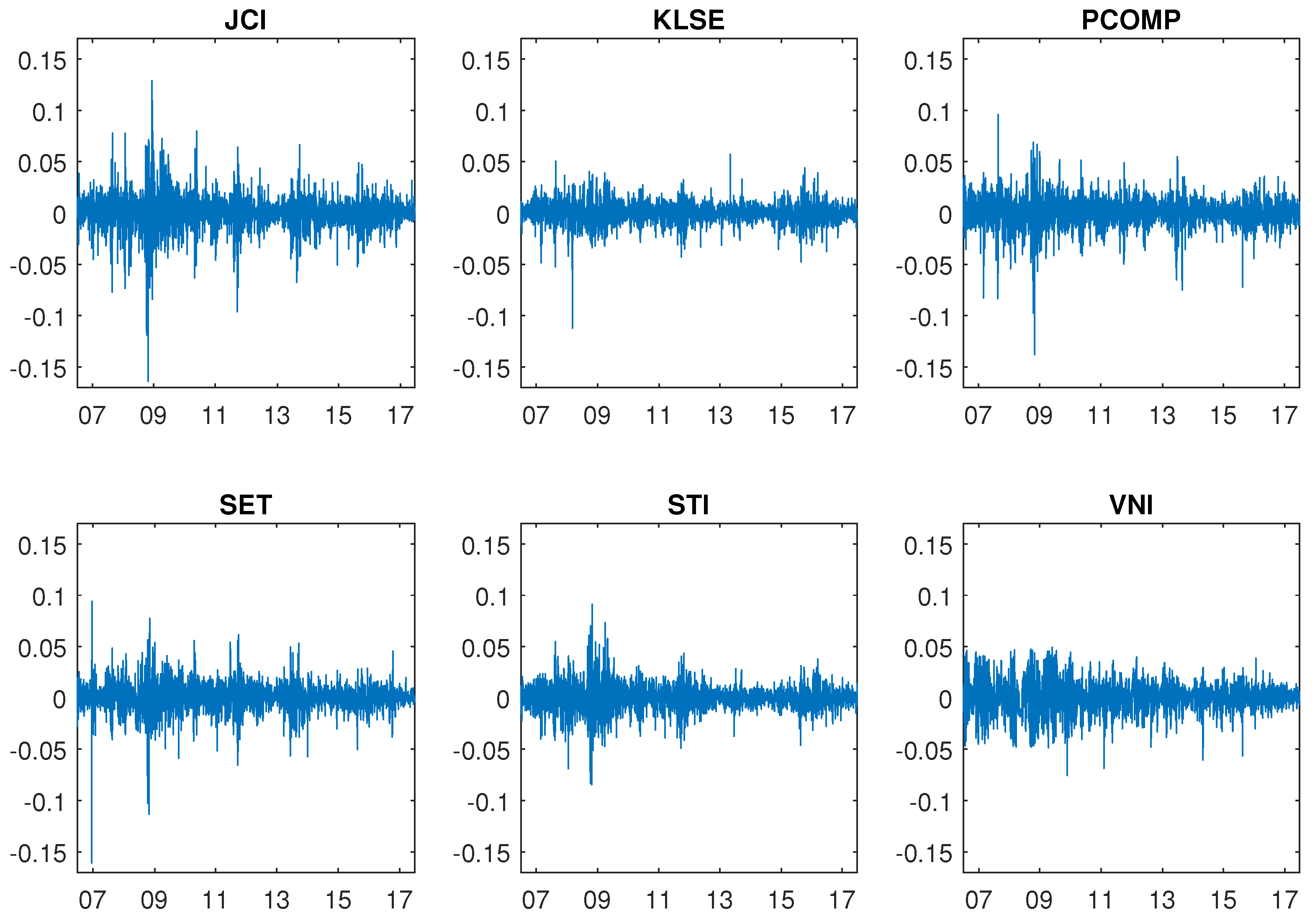
Figure 2.
Value-at-Risk () 1-day ahead forecast with Historical Simulation for the SET index.

Table 1.
Descriptive statistics of the log-returns for the six ASEAN stock indices in the period 1 July 2006–30 June 2017. Rejection of the null-hypothesis is displayed with asterisks (* 1% level of significance).
Table 1.
Descriptive statistics of the log-returns for the six ASEAN stock indices in the period 1 July 2006–30 June 2017. Rejection of the null-hypothesis is displayed with asterisks (* 1% level of significance).
| Obs. | Mean | Min. | Max. | Std. Dev. | Skewn. | Kurtosis | LB(12) | ARCH(12) | ADF | |
|---|---|---|---|---|---|---|---|---|---|---|
| JCI | 2674 | 0.0413 | −16.3976 | 12.8918 | 1.5024 | −0.5791 | 12.5428 | 58.6283 * | 414.1944 * | −46.7885 * |
| KLSE | 2683 | 0.0493 | −13.7896 | 9.5896 | 1.4425 | −0.7345 | 10.2419 | 69.4031 * | 354.3988 * | −45.7856 * |
| PCOMP | 2709 | 0.0152 | −11.2295 | 5.7262 | 1.0244 | −0.5489 | 10.5371 | 34.8944 * | 96.5796 * | −46.7559 * |
| SET | 2687 | 0.0353 | −16.0911 | 9.4139 | 1.3997 | −0.9414 | 15.2982 | 41.0240 * | 308.1694 * | −49.2268 * |
| STI | 2761 | 0.0158 | −8.4502 | 9.1221 | 1.2931 | −0.1834 | 8.5997 | 51.0448 * | 845.2581 * | −49.7627 * |
| VNI | 2737 | 0.0027 | −7.5612 | 4.9411 | 1.5211 | −0.2330 | 4.4559 | 210.0781 * | 604.1086 * | −40.7110 * |
Note: Obs. is the number of observations, Min. and Max. are the minimum and maximum return in the sample, Std. Dev. is the standard deviation, LB(12) refers to the Ljung-Box test with 12 lags, ARCH(12) refers to the ARCH test for heteroskedasticity at 12 lags and ADF is the augmented Dickey-Fuller test.
Table 2.
Value-at-Risk backtest results for JCI returns.
| Model | Traffic Light | Christoffersen (1998) | Pérignon and Smith (2008) | ||||||||||
| 1% | 2.5% | 5% | |||||||||||
| 1-Day | 5-Days | 20-Days | 1-Day | 5-Days | 20-Days | 1-Day | 5-Days | 20-Days | 1-Day | 5-Days | 20-Days | ||
| long trading position | |||||||||||||
| EWMA/RiskMetrics | 91/1120/0 | − | − | − | − | − | − | − | − | − | − | − | − |
| Historical Simulation | 755/456/0 | − | − | − | − | − | − | − | − | − | 0.2996 | 0.3007 | 0.3053 |
| Filtered Historical Simulation | 1211/0/0 | 0.0740 | − | 0.0868 | 0.1526 | − | − | 0.2174 | − | − | 0.2758 | − | − |
| GARCH-SkSt | 1211/0/0 | − | − | − | − | − | − | − | − | − | − | − | − |
| APARCH-SkSt | 1211/0/0 | 0.0828 | − | − | − | − | − | − | − | − | 0.2469 | − | − |
| FIGARCH-SkSt | 758/453/0 | 0.1047 | − | − | 0.1635 | 0.1526 | − | 0.2385 | − | − | 0.3075 | 0.3007 | 0.3173 |
| FIAPARCH-SkSt | 1173/38/0 | 0.0828 | − | − | − | − | − | − | − | − | − | − | − |
| SV | 653/558/0 | 0.1111 | − | − | 0.1813 | − | − | 0.2297 | − | − | 0.3130 | 0.2961 | 0.2695 |
| SV-t | 362/849/0 | − | − | − | 0.1696 | 0.1571 | − | 0.2312 | − | − | 0.3141 | − | − |
| SV-L | 627/584/0 | 0.1141 | − | − | 0.1526 | − | − | 0.2205 | 0.2110 | − | 0.2914 | 0.2733 | − |
| short trading position | |||||||||||||
| EWMA/RiskMetrics | 847/364/0 | 0.1110 | − | − | 0.1655 | 0.1736 | − | 0.2126 | 0.2174 | 0.2174 | 0.2914 | − | − |
| Historical Simulation | 961/250/0 | 0.0979 | − | − | − | − | − | − | − | − | 0.2891 | 0.2891 | 0.2926 |
| Filtered Historical Simulation | 946/265/0 | 0.0907 | − | − | − | − | − | − | − | − | − | − | − |
| GARCH-SkSt | 1211/0/0 | − | − | − | − | − | − | − | − | − | − | − | − |
| APARCH-SkSt | 1019/192/0 | 0.0907 | 0.1047 | 0.0944 | − | − | 0.1434 | − | − | − | − | 0.2669 | − |
| FIGARCH-SkSt | 926/285/0 | 0.1079 | − | − | 0.1716 | − | − | 0.2427 | − | − | 0.3162 | − | − |
| FIAPARCH-SkSt | 1025/186/0 | 0.0907 | 0.0868 | 0.0828 | − | − | − | − | − | − | − | − | − |
| SV | 1211/0/0 | 0.0740 | − | − | − | − | − | − | − | − | − | − | − |
| SV-t | 1211/0/0 | 0.0785 | 0.0868 | − | − | − | − | − | − | − | − | − | − |
| SV-L | 1152/59/0 | 0.0785 | 0.0828 | − | − | − | − | − | − | − | − | − | − |
Note: Numbers under the Basel traffic light test indicate the number of days in the green/yellow/red zone for a 250 rolling trading day window with 1-day ahead VaR forecasts at . For the Christoffersen (1998) test the 1-, 5-, and 20-days ahead forecasts results are reported for the , , and VaR. If a specific test does not reject the null hypothesis, we present the corresponding VaR loss function result. − indicates that the null hypothesis is rejected at least at 10% level of significance. Bold faced loss functions represent the inclusion in the Model Confidence Set (Hansen et al. 2011) with level of significant 10% and 10,000 bootstraps. The test by Pérignon and Smith (2008) is reported in a similar manner, except for the fact that the three VaR levels (1%, 2.5%, and 5%) are tested jointly.
Table 3.
Value-at-Risk backtest results for KLSE returns.
| Model | Traffic Light | Christoffersen (1998) | Pérignon and Smith (2008) | ||||||||||
| 1% | 2.5% | 5% | |||||||||||
| 1-Day | 5-Days | 20-Days | 1-Day | 5-Days | 20-Days | 1-Day | 5-Days | 20-Days | 1-Day | 5-Days | 20-Days | ||
| long trading position | |||||||||||||
| EWMA/RiskMetrics | 195/925/104 | − | − | − | − | − | − | − | − | − | − | − | − |
| Historical Simulation | 679/545/0 | − | − | − | − | − | − | − | − | − | 0.3159 | 0.3181 | 0.3234 |
| Filtered Historical Simulation | 569/655/0 | 0.1136 | − | 0.1074 | − | 0.1519 | − | 0.2180 | − | − | 0.3016 | 0.2708 | − |
| GARCH-SkSt | 974/250/0 | 0.0864 | 0.0939 | 0.0903 | 0.1542 | − | 0.1474 | 0.2101 | − | − | 0.2745 | − | − |
| APARCH-SkSt | 1034/190/0 | 0.0903 | − | 0.1009 | 0.1627 | 0.1519 | − | 0.2117 | − | − | 0.2818 | 0.2842 | − |
| FIGARCH-SkSt | 523/701/0 | − | − | − | − | − | − | − | − | − | 0.3337 | − | − |
| FIAPARCH-SkSt | 1139/85/0 | 0.0864 | 0.1009 | 0.0782 | 0.1519 | − | − | − | − | − | − | − | − |
| SV | 468/756/0 | − | − | 0.1009 | 0.1786 | − | − | 0.2316 | − | − | 0.3159 | 0.3039 | 0.2695 |
| SV-t | 670/554/0 | − | − | − | 0.1767 | − | − | 0.2374 | − | − | 0.3181 | 0.3170 | 0.2794 |
| SV-L | 750/474/0 | − | − | − | 0.1767 | 0.1606 | − | 0.2286 | − | − | 0.3105 | 0.2994 | 0.2733 |
| short trading position | |||||||||||||
| EWMA/RiskMetrics | 890/334/0 | 0.1074 | 0.1106 | 0.1194 | 0.1497 | 0.1519 | 0.1668 | 0.2117 | 0.2117 | 0.2226 | 0.2806 | 0.2830 | 0.3027 |
| Historical Simulation | 792/353/79 | 0.1165 | − | − | 0.1648 | − | − | − | − | − | 0.3005 | 0.3072 | − |
| Filtered Historical Simulation | 735/402/87 | − | 0.1194 | − | − | − | − | 0.2444 | − | − | − | 0.3061 | − |
| GARCH-SkSt | 969/255/0 | 0.0940 | 0.0864 | 0.0864 | − | − | − | − | − | − | − | − | − |
| APARCH-SkSt | 1046/178/0 | 0.0940 | 0.0782 | 0.0824 | − | − | − | − | − | − | − | − | − |
| FIGARCH-SkSt | 974/250/0 | 0.0975 | 0.0975 | 0.1106 | 0.1648 | 0.1563 | − | 0.2241 | 0.2241 | 0.2286 | 0.2948 | 0.2902 | 0.3072 |
| FIAPARCH-SkSt | 1059/165/0 | 0.0824 | − | − | − | − | − | − | − | − | − | − | − |
| SV | 1046/178/0 | 0.0903 | 0.0824 | − | − | − | − | − | − | − | − | − | − |
| SV-t | 1059/165/0 | 0.0824 | 0.0782 | − | − | − | − | − | − | − | − | − | − |
| SV-L | 1216/8/0 | 0.0864 | 0.0737 | − | − | − | − | − | − | − | − | − | − |
Note: Numbers under the Basel traffic light test indicate the number of days in the green/yellow/red zone for a 250 rolling trading day window with 1-day ahead VaR forecasts at . For the Christoffersen (1998) test the 1-, 5-, and 20-days ahead forecasts results are reported for the , , and VaR. If a specific test does not reject the null hypothesis, we present the corresponding VaR loss function result. − indicates that the null hypothesis is rejected at least at 10% level of significance. Bold faced loss functions represent the inclusion in the Model Confidence Set (Hansen et al. 2011) with level of significant 10% and 10,000 bootstraps. The test by Pérignon and Smith (2008) is reported in a similar manner, except for the fact that the three VaR levels (1%, 2.5%, and 5%) are tested jointly.
Table 4.
Value-at-Risk backtest results for PCOMP returns.
| Model | Traffic Light | Christoffersen (1998) | Pérignon and Smith (2008) | ||||||||||
| 1% | 2.5% | 5% | |||||||||||
| 1-Day | 5-Days | 20-Days | 1-Day | 5-Days | 20-Days | 1-Day | 5-Days | 20-Days | 1-Day | 5-Days | 20-Days | ||
| long trading position | |||||||||||||
| EWMA/RiskMetrics | 216/996/0 | − | − | − | − | − | − | − | − | − | − | − | − |
| Historical Simulation | 968/244/0 | − | − | − | − | − | − | − | − | − | 0.2972 | 0.3040 | 0.3107 |
| Filtered Historical Simulation | 1017/195/0 | 0.0906 | − | − | 0.1716 | − | − | − | − | − | 0.2972 | 0.2719 | 0.2757 |
| GARCH-SkSt | 1003/209/0 | 0.0785 | − | − | − | − | − | − | − | − | − | − | − |
| APARCH-SkSt | 1035/177/0 | − | − | − | 0.1360 | − | − | 0.2044 | − | − | 0.2550 | − | − |
| FIGARCH-SkSt | 554/658/0 | 0.1199 | − | − | 0.1775 | − | − | − | − | − | 0.3289 | 0.3340 | − |
| FIAPARCH-SkSt | 1043/169/0 | 0.0785 | − | − | − | − | − | − | − | − | − | − | − |
| SV | 661/551/0 | 0.1141 | − | − | − | − | − | 0.2384 | − | − | 0.3118 | 0.2890 | − |
| SV-t | 767/445/0 | 0.1047 | − | − | − | − | − | 0.2326 | − | − | 0.3051 | 0.2914 | − |
| SV-L | 916/296/0 | 0.0979 | − | − | 0.1433 | − | − | 0.2158 | − | − | 0.2769 | 0.2732 | − |
| short trading position | |||||||||||||
| EWMA/RiskMetrics | 983/229/0 | 0.1013 | − | − | − | − | − | − | − | − | 0.2769 | − | − |
| Historical Simulation | 717/495/0 | − | − | − | − | − | − | − | − | − | 0.2960 | 0.3029 | − |
| Filtered Historical Simulation | 613/599/0 | 0.1199 | − | − | − | − | − | − | − | − | − | 0.3161 | − |
| GARCH-SkSt | 1212/0/0 | − | − | − | − | − | − | − | − | − | − | − | − |
| APARCH-SkSt | 1109/103/0 | − | − | − | − | − | − | − | − | − | − | − | − |
| FIGARCH-SkSt | 1009/203/0 | 0.0979 | − | − | − | 0.1696 | − | − | − | − | 0.3051 | 0.3073 | − |
| FIAPARCH-SkSt | 1109/103/0 | − | − | − | − | − | − | − | − | − | − | − | − |
| SV | 1109/103/0 | − | − | − | − | − | − | − | − | − | − | − | − |
| SV-t | 1212/0/0 | − | − | − | − | − | − | − | − | − | − | − | − |
| SV-L | 1109/103/0 | − | − | − | − | − | − | − | − | − | − | − | − |
Note: Numbers under the Basel traffic light test indicate the number of days in the green/yellow/red zone for a 250 rolling trading day window with 1-day ahead VaR forecasts at . For the Christoffersen (1998) test the 1-, 5-, and 20-days ahead forecasts results are reported for the , , and VaR. If a specific test does not reject the null hypothesis, we present the corresponding VaR loss function result. − indicates that the null hypothesis is rejected at least at 10% level of significance. Bold faced loss functions represent the inclusion in the Model Confidence Set (Hansen et al. 2011) with level of significant 10% and 10,000 bootstraps. The test by Pérignon and Smith (2008) is reported in a similar manner, except for the fact that the three VaR levels (1%, 2.5%, and 5%) are tested jointly.
Table 5.
Value-at-Risk backtest results for SET returns.
| Model | Traffic Light | Christoffersen (1998) | Pérignon and Smith (2008) | ||||||||||
| 1% | 2.5% | 5% | |||||||||||
| 1-Day | 5-Days | 20-Days | 1-Day | 5-Days | 20-Days | 1-Day | 5-Days | 20-Days | 1-Day | 5-Days | 20-Days | ||
| long trading position | |||||||||||||
| EWMA/RiskMetrics | 387/738/95 | − | − | − | − | − | − | 0.2363 | − | − | − | − | − |
| Historical Simulation | 699/521/0 | 0.1167 | − | − | 0.1630 | − | − | 0.2199 | − | 0.2260 | 0.2975 | 0.3032 | 0.3032 |
| Filtered Historical Simulation | 814/345/61 | 0.1167 | − | − | 0.1650 | − | − | 0.2290 | − | − | 0.3054 | − | − |
| GARCH-SkSt | 1009/211/0 | 0.0825 | − | − | − | − | − | − | − | − | − | − | − |
| APARCH-SkSt | 978/242/0 | 0.0904 | 0.0976 | 0.0865 | 0.1521 | 0.1453 | − | 0.2104 | − | − | 0.2749 | − | − |
| FIGARCH-SkSt | 613/607/0 | 0.1224 | − | − | − | − | − | − | − | 0.2245 | − | − | − |
| FIAPARCH-SkSt | 1159/61/0 | 0.0825 | 0.1076 | 0.0941 | 0.1381 | 0.1429 | − | 0.2071 | − | − | 0.2622 | − | 0.2557 |
| SV | 620/600/0 | 0.1107 | − | 0.0904 | 0.1808 | − | − | 0.2391 | − | − | 0.3196 | − | − |
| SV-t | 732/488/0 | 0.1107 | 0.1076 | 0.0904 | 0.1826 | 0.1566 | − | 0.2475 | − | − | 0.3269 | 0.2929 | 0.2583 |
| SV-L | 1015/205/0 | 0.0865 | 0.1076 | 0.0865 | 0.1608 | 0.1587 | − | 0.2245 | − | − | 0.2894 | 0.2858 | − |
| short trading position | |||||||||||||
| EWMA/RiskMetrics | 629/591/0 | − | − | − | − | − | − | − | − | − | − | − | − |
| Historical Simulation | 760/460/0 | − | − | − | − | − | − | − | − | − | 0.2798 | 0.2798 | 0.2858 |
| Filtered Historical Simulation | 759/461/0 | − | − | − | − | − | − | − | − | − | 0.3196 | 0.2648 | − |
| GARCH-SkSt | 1018/202/0 | − | − | − | − | − | − | − | − | − | − | − | − |
| APARCH-SkSt | 1220/0/0 | − | − | − | − | − | − | − | − | − | − | − | − |
| FIGARCH-SkSt | 1043/177/0 | − | − | − | − | − | − | − | − | − | 0.2774 | 0.2774 | − |
| FIAPARCH-SkSt | 990/230/0 | − | − | − | − | − | − | − | − | − | − | − | − |
| SV | 1220/0/0 | − | − | − | − | − | − | − | − | − | − | − | − |
| SV-t | 1146/74/0 | − | − | − | − | − | − | − | − | − | − | − | − |
| SV-L | 1220/0/0 | − | − | − | − | − | − | − | − | − | − | − | − |
Note: Numbers under the Basel traffic light test indicate the number of days in the green/yellow/red zone for a 250 rolling trading day window with 1-day ahead VaR forecasts at . For the Christoffersen (1998) test the 1-, 5-, and 20-days ahead forecasts results are reported for the , , and VaR. If a specific test does not reject the null hypothesis, we present the corresponding VaR loss function result. − indicates that the null hypothesis is rejected at least at 10% level of significance. Bold faced loss functions represent the inclusion in the Model Confidence Set (Hansen et al. 2011) with level of significant 10% and 10,000 bootstraps. The test by Pérignon and Smith (2008) is reported in a similar manner, except for the fact that the three VaR levels (1%, 2.5%, and 5%) are tested jointly.
Table 6.
Value-at-Risk backtest results for STI returns.
| Model | Traffic Light | Christoffersen (1998) | Pérignon and Smith (2008) | ||||||||||
| 1% | 2.5% | 5% | |||||||||||
| 1-Day | 5-Days | 20-Days | 1-Day | 5-Days | 20-Days | 1-Day | 5-Days | 20-Days | 1-Day | 5-Days | 20-Days | ||
| long trading position | |||||||||||||
| EWMA/RiskMetrics | 234/1004/17 | − | − | − | − | − | − | − | − | − | − | − | − |
| Historical Simulation | 830/425/0 | − | − | − | 0.1710 | − | − | − | − | − | 0.2996 | 0.2996 | 0.3105 |
| Filtered Historical Simulation | 764/491/0 | 0.0965 | − | − | 0.1651 | − | − | 0.2157 | − | − | 0.2883 | − | − |
| GARCH-SkSt | 1255/0/0 | − | − | − | − | − | − | − | − | − | − | − | − |
| APARCH-SkSt | 895/360/0 | 0.0893 | − | − | 0.1481 | − | − | 0.2014 | − | − | 0.2655 | − | − |
| FIGARCH-SkSt | 628/627/0 | − | − | − | − | − | − | − | − | − | 0.3302 | − | 0.3137 |
| FIAPARCH-SkSt | 950/305/0 | 0.0999 | − | − | 0.1436 | − | − | − | − | − | − | − | − |
| SV | 747/508/0 | − | − | 0.0855 | 0.1768 | − | 0.1436 | 0.2419 | − | − | 0.3221 | 0.3148 | 0.2655 |
| SV-t | 608/647/0 | − | − | − | 0.1710 | − | 0.1504 | 0.2433 | − | − | 0.3221 | 0.3105 | 0.2741 |
| SV-L | 897/358/0 | 0.1031 | − | − | 0.1569 | − | − | 0.2173 | − | − | 0.2871 | − | 0.2473 |
| short trading position | |||||||||||||
| EWMA/RiskMetrics | 1036/219/0 | 0.1094 | 0.1153 | − | 0.1691 | 0.1710 | 0.1691 | 0.2203 | 0.2203 | 0.2203 | 0.2985 | 0.3018 | − |
| Historical Simulation | 729/526/0 | 0.1094 | 0.1124 | 0.1237 | 0.1730 | − | − | − | − | − | 0.2985 | 0.3007 | − |
| Filtered Historical Simulation | 809/387/59 | 0.1209 | 0.0999 | 0.1031 | − | 0.1526 | 0.1590 | 0.2391 | − | − | 0.3252 | − | − |
| GARCH-SkSt | 1255/0/0 | − | − | − | − | − | − | − | − | − | − | − | − |
| APARCH-SkSt | 1030/225/0 | 0.0999 | 0.0965 | 0.0999 | 0.1526 | 0.1481 | 0.1389 | 0.2111 | 0.2047 | − | 0.2789 | 0.2704 | − |
| FIGARCH-SkSt | 619/636/0 | 0.1237 | − | − | − | − | 0.1749 | 0.2277 | 0.2363 | − | − | 0.3221 | 0.3116 |
| FIAPARCH-SkSt | 958/297/0 | 0.1031 | 0.0774 | − | 0.1459 | − | − | − | − | − | 0.2680 | − | − |
| SV | 1237/18/0 | 0.0855 | − | − | − | − | − | − | − | − | − | − | − |
| SV-t | 1117/138/0 | − | − | 0.0729 | − | − | − | 0.1997 | − | − | 0.2500 | − | − |
| SV-L | 1255/0/0 | 0.0774 | − | − | − | − | − | − | − | − | − | − | − |
Note: Numbers under the Basel traffic light test indicate the number of days in the green/yellow/red zone for a 250 rolling trading day window with 1-day ahead VaR forecasts at . For the Christoffersen (1998) test the 1-, 5-, and 20-days ahead forecasts results are reported for the , , and VaR. If a specific test does not reject the null hypothesis, we present the corresponding VaR loss function result. − indicates that the null hypothesis is rejected at least at 10% level of significance. Bold faced loss functions represent the inclusion in the Model Confidence Set (Hansen et al. 2011) with level of significant 10% and 10,000 bootstraps. The test by Pérignon and Smith (2008) is reported in a similar manner, except for the fact that the three VaR levels (1%, 2.5%, and 5%) are tested jointly.
Table 7.
Value-at-Risk backtest results for VNI returns.
| Model | Traffic Light | Christoffersen (1998) | Pérignon and Smith (2008) | ||||||||||
| 1% | 2.5% | 5% | |||||||||||
| 1-Day | 5-Days | 20-Days | 1-Day | 5-Days | 20-Days | 1-Day | 5-Days | 20-Days | 1-Day | 5-Days | 20-Days | ||
| long trading position | |||||||||||||
| EWMA/RiskMetrics | 325/764/159 | − | − | − | − | 0.1809 | − | 0.2268 | − | − | − | − | − |
| Historical Simulation | 1122/126/0 | 0.0731 | 0.0775 | 0.0731 | − | − | − | − | − | − | − | − | − |
| Filtered Historical Simulation | 748/500/0 | 0.0967 | − | − | 0.1529 | − | − | 0.2002 | − | − | 0.2699 | − | − |
| GARCH-SkSt | 1248/0/0 | − | − | − | − | − | − | − | − | − | − | − | − |
| APARCH-SkSt | 872/376/0 | 0.0857 | 0.0967 | − | − | − | − | − | − | − | − | − | − |
| FIGARCH-SkSt | 782/466/0 | 0.1127 | 0.1212 | 0.1185 | 0.1791 | 0.1791 | − | − | 0.2253 | 0.2253 | 0.3155 | 0.3123 | 0.3102 |
| FIAPARCH-SkSt | 1036/212/0 | 0.0775 | − | − | − | − | − | − | − | − | − | − | − |
| SV | 864/384/0 | 0.0967 | 0.0967 | − | 0.1392 | 0.1368 | − | 0.2068 | − | − | 0.2674 | − | − |
| SV-t | 864/384/0 | 0.0967 | 0.0817 | − | 0.1343 | 0.1343 | − | 0.2068 | 0.2002 | − | 0.2649 | 0.2546 | − |
| SV-L | 929/319/0 | 0.0967 | 0.0932 | − | 0.1507 | 0.1368 | − | 0.1968 | − | − | 0.2661 | − | − |
| short trading position | |||||||||||||
| EWMA/RiskMetrics | 965/283/0 | − | − | − | − | − | − | − | − | − | 0.3025 | 0.3176 | − |
| Historical Simulation | 1072/176/0 | 0.0857 | 0.0857 | 0.0817 | − | − | − | − | − | − | 0.2636 | 0.2598 | 0.2546 |
| Filtered Historical Simulation | 845/384/19 | 0.0967 | 0.0731 | − | 0.1485 | − | − | 0.2051 | − | − | 0.2711 | − | − |
| GARCH-SkSt | 1248/0/0 | − | − | − | − | − | − | − | − | − | − | − | − |
| APARCH-SkSt | 1248/0/0 | − | − | − | − | − | − | − | − | − | − | − | − |
| FIGARCH-SkSt | 384/841/23 | − | − | − | − | − | − | − | − | − | − | − | − |
| FIAPARCH-SkSt | 1248/0/0 | − | − | − | − | − | − | − | − | − | − | − | − |
| SV | 1248/0/0 | − | − | − | − | − | − | − | − | − | − | − | − |
| SV-t | 1248/0/0 | − | − | − | − | − | − | − | − | − | − | − | − |
| SV-L | 1248/0/0 | − | − | − | − | − | − | − | − | − | − | − | − |
Note: Numbers under the Basel traffic light test indicate the number of days in the green/yellow/red zone for a 250 rolling trading day window with 1-day ahead VaR forecasts at . For the Christoffersen (1998) test the 1-, 5-, and 20-days ahead forecasts results are reported for the , , and VaR. If a specific test does not reject the null hypothesis, we present the corresponding VaR loss function result. − indicates that the null hypothesis is rejected at least at 10% level of significance. Bold faced loss functions represent the inclusion in the Model Confidence Set (Hansen et al. 2011) with level of significant 10% and 10,000 bootstraps. The test by Pérignon and Smith (2008) is reported in a similar manner, except for the fact that the three VaR levels (1%, 2.5%, and 5%) are tested jointly.
© 2018 by the authors. Licensee MDPI, Basel, Switzerland. This article is an open access article distributed under the terms and conditions of the Creative Commons Attribution (CC BY) license (http://creativecommons.org/licenses/by/4.0/).
Share and Cite
MDPI and ACS Style
Bui Quang, P.; Klein, T.; Nguyen, N.H.; Walther, T. Value-at-Risk for South-East Asian Stock Markets: Stochastic Volatility vs. GARCH. J. Risk Financial Manag. 2018, 11, 18. https://doi.org/10.3390/jrfm11020018
AMA Style
Bui Quang P, Klein T, Nguyen NH, Walther T. Value-at-Risk for South-East Asian Stock Markets: Stochastic Volatility vs. GARCH. Journal of Risk and Financial Management. 2018; 11(2):18. https://doi.org/10.3390/jrfm11020018
Chicago/Turabian StyleBui Quang, Paul, Tony Klein, Nam H. Nguyen, and Thomas Walther. 2018. "Value-at-Risk for South-East Asian Stock Markets: Stochastic Volatility vs. GARCH" Journal of Risk and Financial Management 11, no. 2: 18. https://doi.org/10.3390/jrfm11020018