Forecasting of Realised Volatility with the Random Forests Algorithm

Abstract

The paper addresses the forecasting of realised volatility for financial time series using the heterogeneous autoregressive model (HAR) and machine learning techniques. We consider an extended version of the existing HAR model with included purified implied volatility. For this extended model, we apply the random forests algorithm for the forecasting of the direction and the magnitude of the realised volatility. In experiments with historical high frequency data, we demonstrate improvements of forecast accuracy for the proposed model.

1. Introduction

In this paper, the estimation of historical volatility is considered for financial time series generated by stock prices and indexes. This estimation is a necessary step for the volatility forecast which is crucial for the pricing of financial derivatives and for optimal portfolio selection. The methods of estimation and forecast of volatility have been intensively studied (see, e.g., the references in Andersen and Bollerslev (1997) and in De Stefani et al. (2017); Dokuchaev (2014)).

In pricing of derivatives, option traders use volatility as the input for determining the value of an option using underlying models such as the Black–Scholes’ (Black and Scholes 1973) and Heston’s (1993) option pricing models. Hence, being able to forecast the direction and magnitude of the future volatility on different time horizons will provide advantages in terms of pricing risks and the development of trading strategies.

There is an enormous body of research on modelling and forecasting volatility. Engle (1982) and Bollerslev (1986) first proposed the ARCH model and the GARCH model for forecasting volatility. These models have been extended in a number of directions based on the empirical evidences that the volatility process is non-linear, asymmetry, and has a long memory. Such extensions can be referred to EGARCH—Nelson (1991), GJR-GARCH—Glosten et al. (1993), AGARCH—Engle (1990), and TGARCH—Zakoian (1994). However, studies have found that those models cannot describe the whole-day volatility information well enough because they were developed within low-frequency time sequences.

With the appearance of high-frequency data, Andersen et al. (2003) introduced a new volatility measure. This proxy was known as realized volatility (RV). In comparison with the GARCH-type measures, realised volatility is preferred as it is a model-free measure. Hence, it provides convenience for calculation. In addition, the realised volatility takes high-frequency data into consideration and exhibits the long memory property. There have been many forecasting models that have been developed to predict the realised volatility. Among those models, the heterogeneous autogressive model for realised volatility (HAR) by Corsi (2003) is one to name. The HAR-RV model was developed in accordance with the heterogeneous market hypothesis proposed by Muller et al. (1997) and the long memory character of realised volatility by Andersen et al. (2003). Empirical studies have shown that the HAR model has high forecasting performance for future volatility, especially for out-of-sample data with different time horizons (Corsi 2003; Khan 2011).

Another commonly used volatility measure is the implied volatility. The implied volatility is often derived from the observed market option prices and is regarded as the fear gauge Whaley (2000). The implied volatility fluctuates with stock movement, strike price, interest rate, time-to-maturity, and option price. To reduce the impact of stock price movement, a so-called “purified” implied volatility was introduced in Luong and Dokuchaev (2014). In the present paper, we show that that this volatility measure contains some information about the future volatility.

To produce rules for prediction for the classes and the regression of the outcome variables, classification and regression tree models and other machine learning techniques have been developed in the literature (see the references in De Stefani et al. (2017)). This paper explores the related random forests algorithm to improve the forecasting of realised volatility in the machine learning setting.

This algorithm is constructed to predict both the direction and the magnitude of realised volatility, based on the HAR model framework with the inclusion of the purified implied volatility.

The paper is structured as follows. In Section 2, we provide the background of the volatility measures, the classical HAR model, and the random forests algorithm. We then discuss our proposed model and methodology and their results in Section 3. Section 4 provides discussion of the study, and we conclude the results of this study in Section 5.

2. Materials and Methods

2.1. Random Forests Algorithm

Breiman (2001) introduced the random forests (RF) algorithm as an ensemble approach that can also be thought of as a form of nearest neighbour predictor. The random forest starts with a standard machine learning technique called “decision trees”. We provide a brief summary of this algorithm in this section.

2.1.1. Decision Trees

The decision trees algorithm is an approach that uses a set of binary rules to calculate a target class or value. Different from predictors like linear or polynomial regression where a single predictive formula is supposed to hold over the entire data space, decision trees aim to sub-divide the data into multiple partitions using a recursive method, and then fit simple models to each cell of the partition. Each decision tree has three levels:

• Root nodes: entry points to a collection of data;
• Inner nodes: a set of binary questions where each child node is available for every possible answer;
• Leaf nodes: respond to the decision to take if reached.

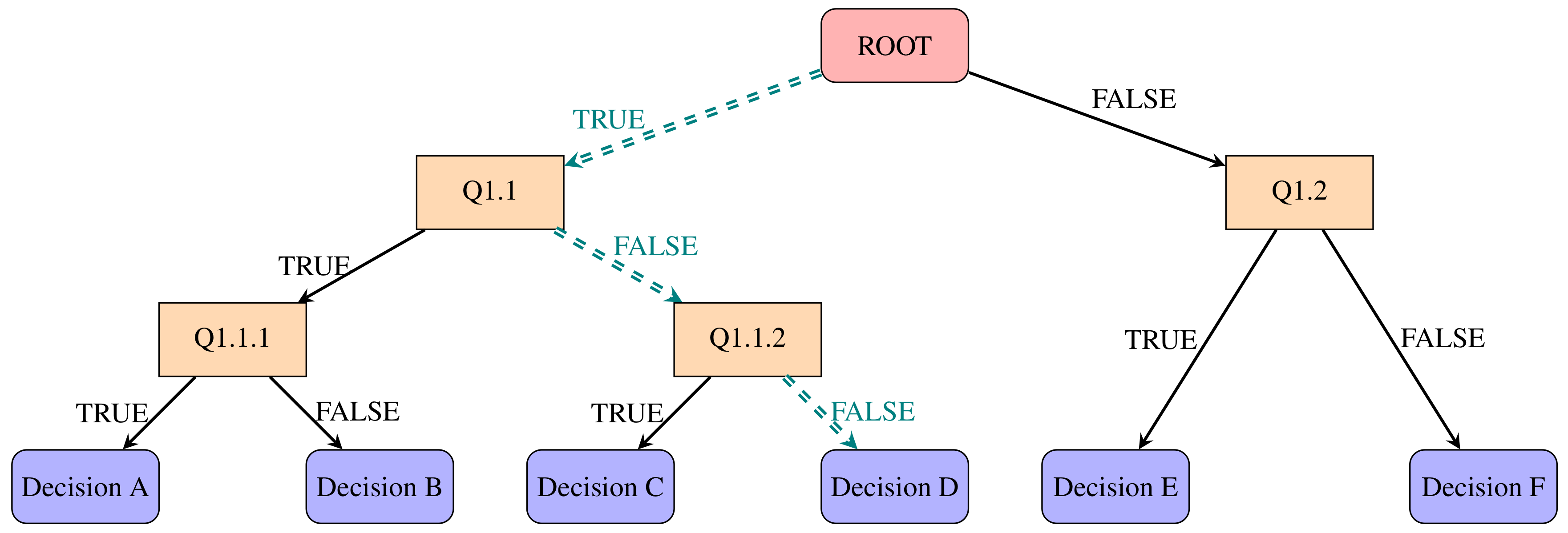
For example, in order to predict a response or class Y from inputs $X_1,X_2,...,X_n$, a binary tree is constructed based on the information from each input. At the internal nodes in the tree, a test to one of the inputs is run for a given criterion with logical outcomes: TRUE or FALSE. Depending on the outcome, a decision is drawn to the next sub-branches corresponding to the TRUE or FALSE response. Eventually, a final prediction outcome is obtained at the leaf node. This prediction aggregates or averages all of the training data points which reach that leaf. Figure 1 illustrates the binary tree concept.

Algorithm 1 describes how a decision tree can be constructed using CART from (Breiman et al. 1984). This algorithm is computationally simple and quick to fit the data. In addition, as it requires no parametric, no formal distributional assumptions are required. However, one of the main disadvantages of tree-based models is that they exhibit instability and high variance, i.e., a small change in the data can result in a very different series of split, or over-fitting. To overcome such a major issue, we used an alternative ensemble approach known as the random forests algorithm.

Algorithm 1: Classification And Regression Trees - CART algorithm for building decision trees.

1: Let N be the root node with all available data.

2: Find the feature F and threshold value T that split the samples assigned to N into subsets

$I_{TRUE}$ and $I_{FALSE}$, to maximise the label purity within these subsets.

3: Assign the pair (F, T) to N.

4: If $I\left(s\right)$ is too small to be split, attach a ‘child’ leaf node to $L_{TRUE}$ and $L_{FALSE}$ to N and

assign the leaves with the most present label in $I_{TRUE}$ and $I_{FALSE}$, respectively.

If subset $I\left(s\right)$ is large enough to be split, attach child nodes $N_{TRUE}$ and $N_{FALSE}$ to N,

and then assign $I\left(s\right)$ to them, respectively.

5: Repeat steps 2–4 for the new nodes $N=N_{TRUE}$ and $N=N_{FALSE}$ until the new subsets

can no longer be split.

2.1.2. Random Forests

A random forest can be considered to be a collection or ensemble of simple decision trees that are selected randomly. It belongs to the class of so-called bootstrap aggregation or bagging technique which aims to reduce the variance in an estimated prediction function. Particularly, a number of decision trees are constructed and random forests will either “vote” for the best decision (classification problems) or “average” the predicted values (regression problems). Here, each tree in the collection is formed by firstly selecting, at random, at each node, a small group of input coordinates (also called features or variables hereafter) to split on and secondly, by calculating the best split based on these features in the training set. The tree is grown using the CART algorithm to maximum size, without pruning. The use of random forests can lead to significant improvements in prediction accuracy (i.e., better ability to predict new data cases) in comparison with a single decision tree, as discussed in the previous section. Algorithm 2 from Breiman (2001) details how the random forests can be constructed.

For $m=1$, the algorithm uses random splitter selection. m can also be set to the total number of predictor variables which is known as Breiman’s bagger parameter (Breiman 2001). In this paper, we set m as equal to the maximum number of variables of interest used in the proposed model.

Applications of the random forests algorithm can be found in machine learning, pattern recognitions, bio-infomatics, and big data modelling. Recently, a number of financial literatures have applied the random forests algorithm to the forecasting of stock prices as well as in developing the investment strategies found in Theofilatos et al. (2012) and Qin et al. (2013). Here, we introduce an application of the random forests algorithm involving the forecasting of the realised volatility.

Algorithm 2: Random forests

1: Draw a number of bootstrap samples from the original data ($n_{tree}$) to be grown.

2: Sample N cases at random with replacement to create a subset of the data. The subset is

then split into in-bag and out-of-bag samples at a selected ratio (i.e., 7:3).

3: At each node, for a preselected number m, m predictor variables ($m_{try}$) are chosen at

random from all the predictor variables.

4: The predictor variable that provides the best split, according to some objective function,

is used to build a binary split on that node.

5: At the next node, choose another m variables at random from all predictor variables.

6: Repeat 3–5 until all nodes are grown.

2.2. Volatility Measures

Volatility, often measured by the standard deviation or variance of returns from a financial security or market index, is an important component of asset allocation, risk management, and pricing derivatives. In this section, we discuss the two measures of volatility known as the realised volatility and the purified implied volatility.

2.2.1. Realised Volatility

The realised volatility measure was proposed by Andersen et al. (2003) in 2003 based on the use of high frequency data.

Let $S\left(t\right)$ represent the asset price which is observed at equally-spaced discrete points within a given time interval $[t-\delta ,t]$, where $0⩽t-\delta ⩽t⩽T$, $s\left(t\right)=logS\left(t\right)$ and $r(t,\delta )=s\left(t\right)-s(t-\delta )$. We assume that $S\left(t\right)$ is represented by the following Ito equation

$$ds\left(t\right)=\mu \left(t\right)dt+\sigma \left(t\right)dW\left(t\right),0⩽t⩽T,$$

(1)

where $W\left(t\right)$ is a standard Brownian process, $\mu \left(t\right)$ and $\sigma \left(t\right)$ are predictable processes with $\sigma \left(t\right)$ being the standard deviation of $ds\left(t\right)$ and independent of $dW\left(t\right)$. Therefore, the processes $\mu \left(t\right)$ and $\sigma \left(t\right)$ represent the instantaneous conditional mean and volatility of the return. Hence,

$$r(t,\delta )=s\left(t\right)-s(t-\delta )={\int }_{t-\delta }^t\mu \left(\tau \right)d\tau +{\int }_{t-\delta }^t\sigma \left(\tau \right)W\left(t\right).$$

(2)

Following this result, let us assume that the time interval $[t-\delta ,t]$ is observed evenly at Δ steps in discrete time. The realised volatility (RV) of $S\left(t\right)$ can be estimated by

$$R{V}_{t-\delta ,t}=\sqrt{\sum _{j=0}^{M-1}{r}_{t-j\Delta }^2},$$

(3)

where $r_{t-j\Delta }=s(t-j\Delta )-s(t-(j+1)\Delta )$, $\Delta =\frac{1}{M}$, and M is the number of observations within that time interval.

2.2.2. The Purified Implied Volatility

The implied volatility is often known as the ex-ante measure of volatility, and is derived from either the Black–Scholes’ options pricing model from Black and Scholes (1973) (model-based estimation) or from theoptions market price formula by Carr and Wu (2006) (model-free estimation). Such measures depend on several inputs, such as time-to-expiration, stock price, exercise price, risk-free-rate-of-interest, and observed call/put price. Hence, the implied volatility will vary in accordance with the fluctuations of these inputs. In order to reduce the impact of the stock price movements, the purified implied volatility (PV) was introduced in Luong and Dokuchaev (2014). The purified implied volatility is derived from the Black–Scholes options pricing model, where the market option prices are replaced by artificial option prices that reduce the impact of the market price from the observed option prices. The paper also shows that the purified implied volatility does contain information about the traditional volatility measure (i.e., the standard deviation of the low-frequency daily returns). In this paper, we include the purified implied volatility as an extended variable of the HAR model.

2.3. Models for Volatility

2.3.1. Heterogeneous Autoregressive Model for Realised Volatility

Corsi (2003) (see also Corsi and Reno (2009)) proposed the heterogeneous autoregressive model for realised volatility as an extension of the Heterogenous ARCH (HARCH) class of models analysed by Muller et al. (1997), which recognizes the presence of heterogeneity in the traders. The idea stems from the “Fractal Market Hypothesis” (Peters 1994), “Interacting Agent View” (Lux and Marchesi 1999) and “Mixture of Distribution” hypotheses (Andersen and Bollerslev 1997) in the realised volatility process.

It is noted that the definition of realised volatility involves two time parameters: (1) the intraday return interval Δ and (2) the aggregation period one day. For the heterogeneous autoregressive model of realised volatility from Corsi (2003), it is considered that the latent realised volatility is viewed over time horizons longer than one day. The n days historical realised volatility at time t (i.e., $R{V}_{t-n,t}$) is estimated as an average of the daily realised volatility between $(t-n)$ and t. The daily HAR is expressed by

$$R{V}_{t,t+1}={\beta }_0+{\beta }_{D}R{V}_{t-1,t}+{\beta }_{W}R{V}_{t-5,t}+{\beta }_{M}R{V}_{t-22,t}+{\epsilon }_{t,t+1},$$

(4)

where $W=5$ days, $M=22$ days, and $R{V}_{t-5,t},R{V}_{t-22,t}$ present the average realised volatility of the last 5 days and 22 days, respectively. The HAR model can be extended by including the jump component proposed by Barndorff-Nielsen and Shephard (2001) such that

$$\sum _{t-\delta ⩽\tau ⩽t}{J}^2\left(\tau \right)\equiv max\{RV(t-\delta ,t)-BV(t-\delta ,t),0\},$$

(5)

where $BV$ is the realised bi-power variation Barndorff-Nielsen and Shephard (2004). Hence, the general form of the model is

$$R{V}_{t,t+k}={\beta }_0+{\beta }_{D}R{V}_{t-1,t}+{\beta }_{W}R{V}_{t-5,t}+{\beta }_{M}R{V}_{t-22,t}+{\beta }_J{J}_{t-k,t}+{\epsilon }_{t,t+k}.$$

(6)

Most recently, the heterogeneous structure was extended with the inclusion of the leverage effect observed by Black (1976)—the asymmetry in the relationship between returns and volatility noticed by Corsi and Reno (2009). For a given period of time, the leverage level at time t is measured as the average aggregated negative and positive returns during that period where

$$\begin{array}{c}\hfill r_{t-k,t}^{+}=\frac{1}{M}\sum _{j=0}^{M-1}{r}_{t-j\Delta ,t}{I}_{\{r_{t-k,t},\dots ,r_{t,t}⩾0\}};r_{t-k,t}^{-}=\frac{1}{M}\sum _{j=0}^{M-1}{r}_{t-j\Delta ,t}{I}_{\{r_{t-k,t},\dots ,r_{t,t}⩽0\}},\end{array}$$

with M being the number of observations between $t-k$, t, and Δ is the time step. Therefore, one would include the leverage effect as a predictor for the realised volatility in the next k days as follows:

$$\begin{array}{cc}\hfill R{V}_{t,t+k}={\beta }_0& +{\beta }_{D}R{V}_{t-1,t}+{\beta }_{W}R{V}_{t-5,t}+{\beta }_{M}R{V}_{t-22,t}\hfill \\ & +{\beta }_J{J}_{t-k,t}+{\alpha }_P{r}_{t-k,t}^{+}+{\alpha }_N{r}_{t-k,t}^{-}+{\epsilon }_{t,t+k}.\hfill \end{array}$$

(7)

Often, the coefficients ${\beta }_0,{\beta }_D,{\beta }_W,{\beta }_M,{\beta }_J,{\alpha }_P,{\alpha }_N$ are obtained by using the Ordinary-Least-Squares (OLS) estimation for linear regression models.

2.4. The Modified HAR Model for Realised Volatility and Forecasting the Direction

We define two states of the world outcome on the volatility direction as “UP” and “DOWN”. Let $D_{\delta }$ be the direction of the realised volatility observed at the time $\delta$, such that

$$\begin{array}{c}\hfill D_{\delta }=\left\{\begin{array}{cc}UP\hfill & \mathrm{if}{\displaystyle \frac{R{V}_{\delta }}{R{V}_{\delta -1}}}>1,\hfill \\ DOWN\hfill & \mathrm{if}{\displaystyle \frac{R{V}_{\delta }}{R{V}_{\delta -1}}}<1.\hfill \end{array}\right.\end{array}$$

(8)

In order to forecast the direction of realised volatility, a set of predictors (or technical indicators) is used which are derived from the historical price movement of the underlying asset and its realised volatility. Since all available historical information is used, $D_{\delta }$ does not follow a Markov chain. We investigated a number of indicators and through the feature selection process (using variable importance ranking from the random forest algorithm), we found that the following indicators were best for forecasting the realised volatility’s direction.

• The Average True Range (ATR): The ATR is an indicator that measures volatility by using the high–low range of the daily prices. ATR is based on n-periods and can be calculated on an intraday, daily, weekly, or monthly basis. It is noted that ATR is often used as a proxy for volatility. To estimate $AT{R}_t$, we are required to compute the “true range” (TR) such that

  $$T{R}_{\delta }=max\{H_{\delta }-L_{\delta },|H_{\delta }-C_{\delta -1}|,|L-C_{\delta -1}\left|\right\},$$

  (9)

  where $H_{\delta }$, $L_{\delta }$, $C_{\delta -1}$ are the current highest return, the current lowest return, and the previous last return of a selected period, respectively, with absolute values to ensure $T{R}_{\delta }$ is always positive. Hence, the average true range within n-days is

  $$AT{R}_{\delta -n,\delta }=\frac{(n-1)AT{R}_{\delta -n-1,\delta }+T{R}_{\delta }}{n}.$$

  (10)
• Close Relative To Daily Range (CRTDR): The location of the last return within the day’s range is a powerful predictor of next-returns. Here, CRTDR is estimated by

  $$CRTD{R}_{\delta }=\frac{C_{\delta }-L_{\delta }}{H_{\delta }-L_{\delta }},$$

  (11)

  where, $H_{\delta }$, $L_{\delta }$ and $C_{\delta }$ are the high, low, and close returns at time $\delta$ for a selected time period using high frequency returns.
• Exponential Moving Average of realised volatility (EMARV): Exponential moving averages reduce the lag effect in time-series by applying more weight to recent prices. The weighting applied to the most recent price depends on the number of periods (n) in the moving average and the weighting multiplier ($\kappa$). The formula for EMARV of n-periods is as follows:

  $$EMAR{V}_{\delta -n,\delta }=R{V}_{\delta }-\kappa \times EMAR{V}_{\delta -n-1,\delta }+EMAR{V}_{\delta -n-1,\delta }.$$

  (12)
• Moving average convergence/divergence oscillator (MACD) measure of realised volatility: The MACD is one of the simplest and most effective momentum indicators. It turns two moving averages into a momentum oscillator by subtracting the longer moving average (m-days) from the shorter moving average (n-days). The MACD fluctuates above and below the zero line as the moving averages converge, cross, and diverge. We estimate the MACD for realised volatility as

  $$MACDR{V}_{\delta ,m,n}=EMAR{V}_{\delta ,m}-EMAR{V}_{\delta ,n}.$$

  (13)
• Relative Strength Index for realised volatility (RSIRV): This is also a momentum oscillator that measures the speed and change of volatility movements. We define RSIRV as

  $$RSIR{V}_{\delta -n,\delta }=1-{\displaystyle \frac{1}{1+{\displaystyle \frac{{\overline{RV}}_{\delta -n,\delta }^{+}}{{\overline{RV}}_{\delta -n,\delta }^{-}}}}},$$

  (14)

  where ${\overline{RV}}_{\delta -n,\delta }^{+}$ is the average increase in volatility and ${\overline{RV}}_{\delta -n,\delta }^{-}$ is the average decrease in volatility within n-days.

The steps that we take to forecast the volatility direction are listed in Algorithm 3.

Algorithm 3: Forecasting the direction of realised volatility

1: Obtain the direction of the realised volatility.

2: Compute the above technical indicators for each observation.

3: Split the data into a training set and a testing set.

4: Apply the random forests algorithm to the training set to develop the pattern solution of

the realised volatility using the above indicators.

5: Use the solution from Step 4 to predict the direction of the testing set.

Figure 2 demonstrates a possible decision tree that was built for forecasting the direction of realised volatility $D_{\delta }$ using the above steps. In this example, node #4 can be reached when RSI-RV(5) $⩾0.5$ and TR(10) $<0.0084$, with 19% of the in-sample data falling into this category and 91% of these observations being classified as “DOWN”. Likewise, node #27 is reached when RSI-RV(5) $⩽0.5$, $r^{+}⩾0.014$, and $0.0049⩽TR\left(10\right)<0.0072$. In random forests, we can construct similar trees but with different structures to classify the direction of the realised volatility based on the information from other predictors.

Let ${\widehat{D}}_{t,t+k}$ denote the predicted direction of the realised volatility at time $t+k$ using Algorithm 3.

2.5. Forecasting the Realised Volatility—The Proposed Model

To forecast the realised volatility, we consider the heterogeneous autoregression model as discussed in Section 2.3.1. We further include the purified implied volatility and the predicted direction of the future volatility as new predictive variables. Particularly, the model (7) is extended to

$$\begin{array}{cc}R{V}_{t,t+k}=\hfill & {\beta }_0+{\beta }_{D}R{V}_{t-1,t}+{\beta }_{W}R{V}_{t-5,t}+{\beta }_{M}R{V}_{t-22,t}+{\beta }_J{J}_{t-k,t}+{\alpha }_1{r}_{t-k,t}^{+}\hfill \\ & +{\alpha }_2{r}_{t-k,t}^{-}+\gamma P{V}_{t-k,t+22}+\kappa {\widehat{D}}_{t,t+k}+{\epsilon }_{t,t+k}.\hfill \end{array}$$

(15)

We also consider the logarithmic form of this model, as the logarithmic of the realised volatility is often believed to be a smoother process. Thus, we model $logRV$ as

$$\begin{array}{cc}logR{V}_{t,t+k}=\hfill & {\beta }_0+{\beta }_{D}log{RV}_{t-1,t}+{\beta }_{W}log{RV}_{t-5,t}+{\beta }_{M}log{RV}_{t-22,t}+{\beta }_{J}log(1+J_{t-k,t})\hfill \\ & +{\alpha }_{1}log|r_{t-1,t}^{+}|+{\alpha }_{2}log|r_{t-1,t}^{-}|+\gamma log\left(P{V}_{t-k,t+22}\right)+\kappa {\widehat{D}}_{t,t+k}+{\epsilon }_{t,t+k},\hfill \end{array}$$

(16)

where $k=\{1,5,22\}$ for 1-day, 5-day, and 22-day time horizons. We use $log(1+J_{t-k,t})$ instead of $log\left(J_{t-k,t}\right)$ to allow for the cases where $J_{t-k,t}=0$, and the leverage effect is measured by $log|r_{t-1,t}^{*}|$ to allow for the average aggregated negative returns.

The parameters in models (15) and (16) (HAR-JL-PV-D) are fitted using the random forests regression algorithm. It is important to note that for the in-sample data, we replace ${\widehat{D}}_{t,t+k}$ with the actual direction $D_{t,t+k}$ to measure the impact of the direction variable on the forecasting of the realised volatility.

3. The results

3.1. Measuring Errors

Since the paper focuses on forecasting both the realised volatility’s direction and its magnitude, we used the following measures to compare each model.

3.1.1. Classification Problem

In forecasting the direction of the realised volatility, the classification problem consists of only two stages. We measured the accuracy of the forecast as follows.

Let us define the following terms

• True positive (TP): The number of days that are observed with “DOWN” signals that were correctly predicted.
• False positive (FP): The number of days that are observed with “DOWN” signals that were predicted to have “UP” signals.
• False negative (FN): The number of days that are observed with “UP” signals that were predicted to have “DOWN” signals.
• True negative (TN): The number of days that are observed with “UP” signals that were correctly predicted.
• Accuracy: the proportion of the total number of correct predictions

  $$\mathrm{Accuracy}=\frac{TP+TN}{TP+FP+TN+FN}.$$

  (17)

3.1.2. Regression Problem

We split our data into two subsets: the training (in-sample) data and the test (out-of-sample) data. Since we used the random forests algorithm, we measured the accuracy of the model proposed method for training data and test data separately.

Measuring Error for Training Data

For the random forests algorithm, an estimate of the error rate can be obtained based on the training as follows:

• For each bootstrap, predict the out-of-bag values using the tree grown within the bootstrap sample.
• Aggregate the Out-of-bag (OOB) predictions and calculate the mean square error rate by

  $$MS{E}_{OOB}=\frac{1}{m}\sum _{t=1}^n{\left\{R{V}_t-{\overline{R{V}_t}}^{OOB}\right\}}^2$$

  (18)

  where m is the number of observations in the OOB data (i.e., $m<N$) and ${\overline{R{V}_t}}^{OOB}$ is the average of the OOB predictions for the $t^{th}$ observation.
• Estimate the percentage variance explained as a measure of goodness of fit by

  $$1-\frac{MS{E}_{OOB}}{{\sigma }_{RV}^2}$$

  (19)

  where ${\sigma }_{RV}^2$ is the variance in the OOB sample.

Measuring Error for Test Data

Let $R{V}_t$ denote the $t^{th}$ observation, $\widehat{R{V}_t}$ denote its forecast, and k be the number of data points observed in the selected period. The error measures include:

• The mean absolute error

  $$MAE=\frac{1}{k}\sum _{t=1}^k|R{V}_t-\widehat{R{V}_t}|.$$

  (20)
• The mean absolute percentage error

  $$MAPE=\frac{1}{k}\sum _{t=1}^k\frac{|R{V}_t-\widehat{R{V}_t}|}{R{V}_t}.$$

  (21)
• The root mean square error

  $$RMSE=\sqrt{\frac{1}{k}\sum _{t=1}^k{(R{V}_t-\widehat{R{V}_t})}^2}.$$

  (22)
• The root mean square percentage error

  $$RMSPE=\sqrt{\frac{1}{k}\sum _{t=1}^k{\left(\frac{R{V}_t-\widehat{R{V}_t}}{R{V}_t}\right)}^2}.$$

  (23)

3.2. Empirical Results

3.2.1. Data Description

We demonstrate the proposed model by analysing the S&P ASX 200 Index high frequency returns data and their realised volatility. Our dataset was collected from Reuters (2015) for the period 1 January 2008 to 31 December 2014. The Australian Stock Exchange is open between 10:00 a.m. to 4:00 p.m. We collected the tick-by-tick S&P 200 levels; hence, the prices were not recorded at equispaced time points. We used the previous tick aggregation method to force the observed prices into an equispaced grid, i.e., by taking the last price realized before each grid point and obtaining the 15-s frequency data. The daily realised volatility (with 1762 observations) was then estimated using these 15-s prices. The data from 2008 to 2013 were used for training purposes and 2014 data were used for validation purposes. This was to account for over-fitting and bias effects of the time-series data with the random forests algorithm.

The experiment was performed in a cloud-based Linux environment that stored seven years worth of high frequency data. The data aggregation was processed on a 2.5 GHz Intel Xeon Platinum 8175 instance with 32 GB of RAM. The function rxDForest from RevoScaleR package in R was used for the random forests algorithm. This allowed us to effectively handle the large dataset and to execute the computation in parallel. A fixed value of random seed was also set to ensure that the results between each run were comparable and reproducible.

3.2.2. The Results

Below we report the results of our experiment which were the best results obtained via cross-validation and hyper parameter tuning of the rxDForest function.

Table 1. Statistical summary of S&P/ASX 200’s 15-second realised volatility at different time horizons from 1 January 2008 to 31 December 2014 and their correlations matrix.

Series	Mean	Std. Dev.	Skew.	Kurt.	Min.	Max.	${\mathit{RV}}_{\mathit{t}-1,\mathit{t}}$	${\mathit{RV}}_{\mathit{t}-5,\mathit{t}}$	${\mathit{RV}}_{\mathit{t}-22,\mathit{t}}$	PV
$R{V}_{t-1,t}$	0.1335	0.0848	2.4957	8.9530	0.0328	0.7811	1	0.8441	0.7523	0.7757
$R{V}_{t-5,t}$	0.1335	0.0721	2.0481	5.4748	0.0484	0.5453	0.8441	1	0.9042	0.8919
$R{V}_{t-22,t}$	0.1331	0.0664	1.8304	3.9311	0.0593	0.4228	0.7523	0.9042	1	0.9180
PV	0.1614	0.0705	1.5181	2.8461	0.0698	0.5004	0.7757	0.8919	0.9180	1
Series	Mean	Std. Dev	Skew.	Kurt.	Min.	Max.	$\mathbf{log}{\mathit{RV}}_{\mathit{t}-\mathbf{1},\mathit{t}}$	$\mathbf{log}{\mathit{RV}}_{\mathit{t}-\mathbf{5},\mathit{t}}$	$\mathbf{log}{\mathit{RV}}_{\mathit{t}-\mathbf{22},\mathit{t}}$	$\mathbf{log}\mathit{PV}$
$logR{V}_{t-1,t}$	−2.1588	0.5139	0.5678	0.2336	−3.4184	−0.2471	1	0.8548	0.7739	0.7936
$logR{V}_{t-5,t}$	−2.1244	0.4499	0.6619	0.0960	−3.0274	−0.6064	0.8548	1	0.9124	0.8972
$logR{V}_{t-22,t}$	−2.113	0.4213	0.7156	−0.0407	−2.8248	−0.8608	0.7739	0.9124	1	0.9017
$logPV$	−1.9044	0.3893	0.5190	−0.3229	−2.6618	−0.6923	0.7936	0.8972	0.9017	1

provides a summary of the 15-s realised volatility measured using different time-windows. It was observed that both non-logarithmic and logarithmic series are skewed and non-normal. This suggests that the Ordinary Least Squares estimation approach is not applicable for our dataset. As a result, we compared the maximum likelihood estimation (MLE) with the random forests algorithm instead. In terms of correlation coefficients between the series, we observed that the computed realised volatility exhibits the long memory effect. Further, the purified implied volatility was shown to be strongly correlated with the realised volatility measures, which indicates that PV can be a useful predictor of realised volatility.

Table 2. Forecasting error of the realised volatility for the in-sample data from 1 January 2008 to 31 December 2013.

		1-Day				5-Day				22-Day
		HAR-JL	HAR-JL-PV	HAR-JL-D	HAR-JL-PV-D	HAR-JL	HAR-JL-PV	HAR-JL-D	HAR-JL-PV-D	HAR-JL	HAR-JL-PV	HAR-JL-D	HAR-JL-PV-D
RV	RMSE	0.0031	0.0029	0.0018	0.0018	0.002	0.0011	0.0010	0.0010	0.0011	0.0010	0.0009	0.0001
	% OOB Var	57.81	59.61	74.68	75.58	79.28	80.28	81.13	81.81	74.47	76.44	78.09	79.44
log RV	RMSE	0.0996	0.0957	0.0509	0.0502	0.0378	0.0336	0.0326	0.0295	0.0383	0.0323	0.0339	0.0287
	% OOB Var	61.66	63.12	80.39	80.65	80.55	82.70	83.25	84.83	77.48	81.97	80.05	83.12

compares the in-sample forecast results of the proposed model. For the selected time horizons, the inclusion of purified implied volatility improved the forecast accuracy against the original HAR-JL model (based on the RMSE measure and % OOB variance explained), where the logarithmic RV series performed better than the non-logarithmic RV series. It is also observed that the direction indicator further improved the forecast results; this was most significant for the 1-day forecast (with 79.28% and 80.55% variance explained for RV and log RV in comparison with 57.81% and 61.66% from the HAR-JL model respectively). For the 5-day and 22-day in-sample forecasts, we observed slight improvements in RMSE with a better goodness of fit.

In forecasting the direction of the out-sample realised volatility, we obtained the accuracy of the hit-rate at 80.05%, 72.85%, and 65.22% for 1-day, 5-day and 22-day forecasts respectively. This suggests our classification model can perform better for short-term forecasts than long-term forecasts. This can be explained by the fact that long-term forecasts require not only technical indicators but also fundamental indicators and long-term expectations from the market.

Table 3. Forecasing error of the realised volatility for the out-sample data from 1 January 2014 to 31 December 2014.

		1-Day				5-Day				22-Day
		HAR-JL	HAR-JL-PV	HAR-JL-D	HAR-JL-PV-D	HAR-JL	HAR-JL-PV	HAR-JL-D	HAR-JL-PV-D	HAR-JL	HAR-JL-PV	HAR-JL-D	HAR-JL-PV-D
RV	MAE	0.0212	0.0205	0.0176	0.0171	0.0147	0.0135	0.0137	0.0127	0.0184	0.0142	0.017	0.0137
	MAPE	0.2715	0.2516	0.2042	0.1974	0.1814	0.1573	0.1670	0.1500	0.2245	0.1630	0.2094	0.1576
	RMSE	0.0285	0.0277	0.0247	0.0235	0.0192	0.0182	0.0180	0.0168	0.0223	0.0182	0.0209	0.0176
	RMSPE	0.3610	0.3245	0.2709	0.2568	0.2352	0.2025	0.2181	0.1926	0.2745	0.2046	0.2602	0.1973
log RV	MAE	0.0206	0.0201	0.0170	0.0165	0.0143	0.0135	0.0130	0.0129	0.0170	0.0138	0.0156	0.0135
	MAPE	0.2525	0.2331	0.1947	0.1878	0.1740	0.1553	0.1574	0.1481	0.2058	0.1576	0.1881	0.1532
	RMSE	0.0279	0.0280	0.0239	0.0233	0.0185	0.0185	0.0175	0.0175	0.0206	0.0177	0.0191	0.0174
	RMSPE	0.3250	0.2929	0.2573	0.2454	0.2230	0.1980	0.2116	0.1913	0.2499	0.1958	0.2310	0.1912

Note: as the random forests algorithm requires a random selection process, for consistent comparison across models, we reset the random seed to a specific value before applying the algorithm to each of the above models.

provides a summary of the forecast errors for the out-sample data. In general, the out-of-sample performances of the proposed model are in line with the in-sample performances. The MAPE and RMSPE for the 1-day forecast of the RV from the HAR-JL-PV-D reduced by 8% and 11%, respectively, while the MAPE and RMSPE for the 5-day and 22-day forecasts reduced by 3% and 5%. When comparing the HAR-JL-PV model against the HAR-JL-D model, it can be seen that the forecast errors were smaller for the HAR-JL-PV model for these time horizons. This was anticipated as we found that the forecast in the long-term direction was less accurate for the 5-day and 22-day forecasts. However, the HAR-JL-D model still performed better than the HAR-JL alone, and the HAR-JL-PV-D model provided the best fit.

We present in Figure 3 the actual S&P200’s realised volatility measured under different time horizons from 1 January 2014 to 31 December 2014, with the predicted realised volatility using the maximum likelihood estimation for the HAR-JL model (left panel) and using the random forests estimation for the HAR-JL-PV-D model (right panel). Such separation in the time frame was implemented to measure the realised values of our metrics, in order to avoid the over-fitting effect that can possibly be caused by the random forests algorithm.

4. Discussion

Forecasting problems for financial time series are challenging since these series have a significant noise component. Currently, there is no consensus on the possibility of forecasting for asset prices using a technical analysis or a mathematical algorithm. The forecasting of parameters of stochastic models for financial time series, including volatility, is also challenging. Moreover, even statistical inference for parameters of financial time series is usually difficult. An additional difficulty is that these parameters are not directly observable; they are defined by the underlying model and by many other factors. For example, it appears that the volatility depends on the sampling frequency and on the delay parameter in the model equation see, e.g., Luong and Dokuchaev (2016). In addition, there is no a unique comprehensive model for stock price evolution; for example, there are many models with stochastic equations for volatility, with jumps, with fractional noise, etc. Respectively, even a modest improvement in forecasting for the parameters of financial time series would be beneficial for the practitioners.

Our paper explored the HAR (Corsi and Reno 2009) model with the main focus being to extend this model family via two new features, the purified volatility and the forecast volatility movement, and the implementation of this machine learning algorithm to improve the forecast of realised volatility.

By utilising the availability of high frequency data, we showed that the direction of the realised volatility can be forecast with the random forests algorithm by using the proposed technical indicators, with an accuracy of above 80% for the selected time series. However, this accuracy could be further improved if we could integrate fundamental indicators such as financial news.

The errors in forecasting the realised volatility with our proposed features also showed further improvement on top of the existing HAR-JL model. Particularly, this was done through the addition of information derived from the purified volatility and the predicted direction of the volatility. We believe that the predictions of realised volatility would further be improved by using other tree-based algorithms such as Extreme Gradient Boosting (XGBoost) or Bayesian additive regression trees (BART). However, we leave this for future study.

5. Conclusions

This paper introduces an application of the random forests algorithm for forecasting the realised volatility. For the classification problem, our study showed that by using the selected feature choices, it was able to forecast the direction of the realised volatility. For the regression problem with its non-linear structure, the technique was able to reduce the forecasting error rate from volatility clustering systematically under different time horizons. The empirical results of S&P 200 show that the existing HAR model framework was improved by including the purified implied volatility and applying this machine learning technique. We suggest that further investigation of the roles of the purified implied volatility and random forests algorithm in other high frequency models of volatility should be done.

References

- Andersen, Torben G., and Tim Bollerslev. 1997. Heterogeneous information arrivals and return volatility dynamics: Uncovering the long run in high frequency data. Journal of Finance 52: 975–1005. [Google Scholar] [CrossRef]
- Andersen, Torben G., Tim Bollerslev, Francis X. Diebold, and Paul Labys. 2003. Modeling and forecasting realized volatility. Econometrica 71: 529–626. [Google Scholar] [CrossRef]
- Barndorff-Nielsen, Ole E., and Neil Shephard. 2001. Econometric Analysis of Realised Volatility and its Use in Estimating Stochastic Volatility Models. Journal of the Royal Statistical Society 64: 253–80. [Google Scholar] [CrossRef]
- Barndorff-Nielsen, Ole E., and Neil Shephard. 2004. Power and bipower variation with stochastic volatility and jumps. Journal of Financial Econometrics 2: 1–37. [Google Scholar] [CrossRef]
- Black, Fischer, and Myron Scholes. 1973. The Pricing of Options and Corporate Liabilities. Journal of Political Economy 81: 637–54. [Google Scholar] [CrossRef]
- Black, Fischer. 1976. The pricing of commodity contracts. Journal of Financial Economics 3: 167–79. [Google Scholar] [CrossRef]
- Bollerslev, Tim. 1986. Generalized Auto Regressive Conditional Heteroskedasticity. Journal of Econometrics 31: 307–27. [Google Scholar] [CrossRef]
- Breiman, Leo, J. H. Friedman, R. A. Olshen, and C. J. Stone. 1984. Classification and Regression Trees. Monterey: Wadsworth and Brooks. [Google Scholar]
- Breiman, Leo. 2001. Random Forests. Machine Learning 45: 5–32. [Google Scholar] [CrossRef] [Green Version]
- Carr, Peter, and Liuren Wu. 2006. A tale of two indices. Journal of Derivatives 3: 13–29. [Google Scholar] [CrossRef]
- Corsi, Fulvio, and Roberto Reno. 2009. HAR Volatility Modelling With Heterogeneous Leverage and Jumps. Available online: https://web.stanford.edu/group/SITE/archive/SITE_2009/segment_1/s1_papers/corsi.pdf (accessed on 10 October 2018).
- Corsi, Fulvio. 2003. A Simple Approximate Long-Memory Model of Realized Volatility. Journal of Financial Econometrics 7: 174–96. [Google Scholar] [CrossRef]
- De Stefani, Jacopo, Olivier Caelen, Dalila Hattab, and Gianluca Bontempi. 2017. Machine Learning for Multi-step Ahead Forecasting of Volatility Proxies. Available online: https://pdfs.semanticscholar.org/39cf/3536e780ff195d400902076e1b3e7b2e638d.pdf (accessed on 20 September 2015).
- Dokuchaev, Nikolai. 2014. Volatility estimation from short time series of stock prices. Journal of Nonparametric Statistics 26: 373–84. [Google Scholar] [CrossRef]
- Engle, Robert F. 1982. Autoregressive conditional heteroskedasticity with estimates of variance of UK inflation. Econometrica 50: 987–1008. [Google Scholar] [CrossRef]
- Engle, Robert F. 1990. Discussion: Stock market volatility and the crash of 87. Review of Financial Studies 3: 103–6. [Google Scholar] [CrossRef]
- Glosten, Lawrence R., Ravi Jagannathan, and David E. Runkle. 1993. On the relationship between the expected value and the volatility of the nominal excess return on stocks. Journal of Finance 46: 1779–801. [Google Scholar] [CrossRef]
- Heston, Steven L. 1993. A closed-form solution for options with stochastic volatility with applications to bond and currency options. The Review of Financial Studies 6: 327–43. [Google Scholar] [CrossRef]
- Khan, Md Ashraful Islam. 2011. Financial Volatility Forecasting by Nonlinear Support Vector Machine Heterogeneous Autoregressive Model: Evidence from Nikkei 225 Stock Index. International Journal of Economics and Finance 3: 138–50. [Google Scholar] [CrossRef]
- Luong, Chuong, and Nikolai Dokuchaev. 2014. Analysis of market volatility via a dynamically purified option price process. Annals of Financial Economics 9: 1450006. [Google Scholar] [CrossRef]
- Luong, Chuong, and Nikolai Dokuchaev. 2016. Modelling dependency of volatility on sampling frequency via delay equations. Annals of Financial Economics 11: 1650007. [Google Scholar] [CrossRef]
- Lux, Thomas, and Michele Marchesi. 1999. Scaling and criticality in a stochastic multi-agent model of financial market. Nature 397: 498–500. [Google Scholar] [CrossRef]
- Müller, Ulrich A., Michel M. Dacorogna, Rakhal D. Davé, Richard B. Olsen, Olivier V. Pictet, and Jacob E. Von Weizsäcker. 1997. Volatilities of different time resolutions: Analyzing the dynamics of market components. Journal of Empirical Finance 4: 213–39. [Google Scholar] [CrossRef]
- Nelson, Daniel B. 1991. Conditional Heteroskedasticity in Asset Returns: A New Approach. Econometrica 59: 347–70. [Google Scholar] [CrossRef]
- Peters, Edgar. 1994. Fractal Market Analysis. In A Wiley Finance Edition. New York: John Wiley & Sons. [Google Scholar]
- Qin, Qin, Qing-Guo Wang, Jin Li, and Shuzhi Sam Ge. 2013. Linear and Nonlinear Trading Models with Gradient Boosted Random Forests and Application to Singapore Stock Market. Journal of Intelligent Learning Systems and Applications 5: 1–10. [Google Scholar] [CrossRef]
- Reuters, Thomson. 2015. Thomson Reuters Tick History. Available online: http://www.sirca.org.au/ (accessed on 20 September 2015).
- Theofilatos, Konstantinos, Spiros Likothanassis, and Andreas Karathanasopoulos. 2012. Modeling and Trading the EUR/USD Exchange Rate Using Machine Learning Techniques. ETASR—Engineering, Technology & Applied Science Research 2: 269–72. [Google Scholar]
- Whaley, Robert E. 2000. The investor fear gauge. The Journal of Portfolio Management 6: 12–17. [Google Scholar] [CrossRef]
- Zakoian, Jean-Michel. 1994. Threshold Heteroscedastic Models. Journal of Economic Dynamics and Control 18: 931–55. [Google Scholar] [CrossRef]
Figure 1.
A binary tree—starting from the root node, multiple criteria are selected based on the information from each input. A decision is drawn at a particular leaf, i.e., Decision D, if all criteria along its path “==” are satisfied.
Figure 2.
A possible decision tree for classifying the daily realised volatility direction using the technical indicators from the previous day.
Figure 3.
Predicted vs. actual realised volatility using the HAR-JL-PV-D model with the maximum likelihood estimation and random forests estimation.