An Imperfect Production Model for Breakable Multi-Item with Dynamic Demand and Learning Effect on Rework over Random Planning Horizon

Abstract

In recent times, in the literature of inventory management there exists a notorious interest in production-inventory models focused on imperfect production processes with a deterministic time horizon. Nevertheless, it is well-known that there is a high influence and impact caused by the learning effect on the production-inventory models in the random planning horizon. This research work formulates a mathematical model for a re-workable multi-item production-inventory system, in which the demand of the items depends on the accessible stock and selling revenue. The production-inventory model allows shortages and these are partial backlogged over a random planning horizon. Also, the learning effect on the rework policy, inflation, and the time value of money are considered. The main aim is to determine the optimum production rates that minimize the expected total cost of the multi-item production-inventory system. A numerical example is solved and a detailed sensitivity analysis is conducted in order to study the production-inventory model.

1. Introduction

The breakability of the items occurs in the majority of the production-inventory systems. In the fabrication of breakable items, such as televisions, mobiles, fans, watches, among others, the control and regulation are significant parameters to manage effectively and efficiently. Dealing with the mentioned products in production-inventory systems, the breakability becomes in a major problem for the manufacturing companies. In this context, the researchers and practitioners have proposed and implemented inventory models for breakable items in order to make these more practical and realistic. On the other hand, to eliminate waste and reduce the manufacturing cost in real-world production systems, the option of rework plays an important role. The production lot size models with the reworking of defective items are discussed cleverly by Hayek and Salameh (2001); Chiu (2003). To reduce costs being environmentally friendly through reworking plans is studied by Flapper and Teunter (2004). Cost minimizing-planning of work and rework processes for re-workable items is analyzed by Inderfurth et al. (2007). A production model that allows that a certain proportion of defective items can be reworked is reviewed in Chen (2006). Lot sizing models that consider rework, scrap, and maintenance factors are developed by Chiu et al. (2007); Sheu and Chen (2004); Ben-Daya (2002). An economic production quantity (EPQ) model with rework procedure for a single-stage production system under scheduled backorders is proposed by Cardenas-Barron (2009). A non-perfect production stock system with repairing and promotional demand is explored by Manna et al. (2016). In a parallel way, the same year, a production model with rework and multiple deliveries to determine jointly the optimal price, lot size, and the number of deliveries is developed by Taleizadeh et al. (2016). Later, a non-perfect production with advertisement dependent demand and production rate dependent on defective rate is introduced by Manna et al. (2017b). In general, the customers are attracted when the products are displayed in large quantities in the show rooms and this generates a greater demand for them. This makes that the demand be stock-dependent. Perhaps, the first inventory model for stock-dependent consumption rate was done by Gupta and Vrat (1986). Later, Mandal and Phaujdar (1989); Datta and Pal (1990); Pal et al. (1993); Padmanabhan and Vrat (1995) proposed inventory models for stock-dependent demand considering different factors. After that, an inventory model for a power-form inventory-dependent demand pattern was developed by Baker and Urban (1998). A pricing and lot sizing model with partial backlogging for a reseller who vends a consumable item is introduced by Abad (2001). A replenishment stock model with shortages for non-instantaneous deteriorating goods with inventory-dependent demand and partial backlogging is developed by Wu et al. (2006). Additional research works in this area include Dye and Ouyang (2005); Lee and Dye (2012); Avinadav et al. (2013); Taleizadeh et al. (2013). Recently, Debnath et al. (2018) analyzed the effect of delay-in-payment policy and stock-dependent demand in a two-warehouse inventory considering breakable items. Bhunia et al. (2018) proposed an inventory problem for a deteriorating item with displayed stock level and marketing strategy dependent demand. Khanna et al. (2020) determined the optimal preservation strategies in an inventory model with stock-dependent demand and time-dependent holding cost. Banu et al. (2021) considered stock-dependent demand rate in a supply chain model with trade-credit financing. It is important to note that increasing the customer’s demand by lowering the selling price of a commodity also plays an relevant role. Related to this topic, the inventory models in which demand can be increased by decreasing the selling price are formulated by Abad (1996); Lau and Lau (1988); Manna et al. (2017a). Pervin et al. (2019) developed a deteriorating inventory model with stock and price dependent demand for multi-items under the trade-credit policy. Halim et al. (2021) considered stock and nonlinear price-dependent demand in a production-inventory model for deteriorating items. Production-inventory models with and without backlogging are derived using an algebraic method by Cardenas-Barron (2001a, 2001b). Moreover, a pricing and lot-sizing problem for an item with shortages, and partial backlogging are considered in Abad (1996, 2001). A multi-item single-machine manufacturing system considering defective products, partial backlogging and service level constraint is investigated by Taleizadeh et al. (2010). Later, the EOQ/EPQ models with shortages for two varieties of backordering costs, linear and fixed, are deduced by the analytic geometry and the algebraic method in Cardenas-Barron (2011). A non-perfect production-inventory system with preventive maintenance and partial backlogging was derived by Taleizadeh (2017). Nobil et al. (2019) considered shortage, inspection, and rework policy for imperfect items in a production model. Later, Chakraborty et al. (2020) proposed an inventory model for multi-item with multi-warehouse and partial backlogging for perishable goods. AlArjani et al. (2021) developed a sustainable recycle production model with imperfect production and shortages. According to Jaber et al. (2008) the quantity of non-perfect items is reduced due to the learning experience of the system. In this context, an inventory model for non-perfect quality products with shortages taking into account the learning of inspection was described by Konstantaras et al. (2012). Fu et al. (2020) considered learning and fatigue behavioral effects for a labor-intensive production-inventory system. It is well-known that there exists an impact of increasing of prices in the time value of money in today’s monetary market. This is due to the inflation monetary phenomenon, and therefore, this fact can not be ignored in the development of production-inventory models. The research work of Dey et al. (2008) examined the inflation effect and time value of money in a two storage inventory model. Later, Shah and Vaghela (2018) studied the inflation and reliability effects in an imperfect production model for effort and time dependent demand. Shaikh et al. (2020) investigated the effect of inflation and price-dependent demand in a production model for a deteriorating item under trade credit policy. Hemapriya and Uthayakumar (2021) analyzed the inflation and the time value of money effect in a vendor-buyer inventory model.

An overview comparison of existing literature related with the current research work is shown in

Table 1. Comparison of existing literature related with the current research work.

Author(s) (Year)	Model	Learning Effect	Inflation	Backlogging	Demand Rate Depends on	Multi-Item
Mandal and Phaujdar (1989)	Production	No	No	Yes	Stock level	No
Datta and Pal (1990)	Purchase	No	No	No	Stock level	No
Lau and Lau (1998)	Purchase	No	No	Yes	Random	No
Abad (2001)	Purchase	No	No	Yes	Price and time	No
Hayek and Salameh (2001)	Production	No	No	Yes	Constant	No
Ben-Daya (2002)	Production	No	No	No	Time	No
Chiu (2003)	Production	No	No	Yes	Constant	No
Sheu and Chens (2004)	Production	No	No	No	Constant	No
Dye and Ouyang (2005)	Purchase	No	No	Yes	Stock level	No
Wu et al. (2006)	Purchase	No	No	Yes	Stock level	No
Lee and Dye (2012)	Purchase	No	No	Yes	Stock level	No
Avinadav et al. (2013)	Purchase	No	No	No	Price and time	No
Taleizadeh et al. (2013)	Purchase	Yes	No	Yes	Constant	No
Manna et al. (2016)	Production	No	Yes	No	Price and advertisement	Yes
Manna et al. (2017a)	Production	Yes	Yes	Yes	Stock level	Yes
Bhunia et al. (2018)	Purchase	No	No	No	Stock level	No
Pervin et al. (2019)	Supply chain	No	No	No	Price and stock level	Yes
Banu et al. (2021)	Supply chain	No	No	No	Stock level	No
Present paper	Production	Yes, effect on	Yes	Yes	Price and stock level	Yes
		reworked rate

.

This paper develops a multi-item non-perfect production-inventory model with partial backlogging over a finite time horizon in random nature. During the manufacturing period, the screening process and rework process of non-perfect units occur simultaneously. The learning effect is considered where the operator achieves some experience from the previous cycle to increase the rework rate of defective units. The customers’ demand rate is dependent on the displayed inventory level and selling price of the produced items. The effect of inflation and the time value of capital on the total cost of the production-inventory model is analyzed. Based on the random time horizon of the last cycle, four different cases are taking into account. The work is done thru of the following steps:

Step 1

Formulate the imperfect production-inventory model for first $N^j$ fully accommodated cycles considering production, screening, reworking, holding, and shortage costs.

Step 2

Determine the expression of the expected total cost for the first $N^j$ fully accommodated cycles concerning the random time horizon.

Step 3

Calculate the expression of the total cost for the last cycle under the following mutually exclusive and disjoint cases:

–

Case I: The random time horizon ends before the production period concludes.

–

Case II: The random time horizon ends in the between of the end of the production period and exhaust of inventory period.

–

Case III: The random time horizon ends during the shortage period.

–

Case IV: The random time horizon ends during the shortage period when the production restarts to cover the shortages.

Step 4

Compute the expression of the projected total cost for the last period which joins the four mutually exclusive and disjoint events described in Step-3.

Step 5

Minimize the expected total cost including the expressions determined in Step-2 and Step-4.

The remainder of this paper is organized as follows: Section 2 defines the notation and assumptions. Section 3 describes the mathematical formulation of the imperfect production-inventory model. Section 4 presents a numerical example and sensitivity analysis. Section 5 provides practical implications. Finally, Section 6 gives some conclusions and future research directions.

2. Notation and Assumptions

To formulate the imperfect production-inventory model mathematically, the following notation and assumptions are defined.

2.1. Notation

The following notation for $jth$ item ($j=1,2,\dots ,M$) are stated.

$q^j\left(t\right)$	:	Inventory level at time t for perfect quality items in each cycle except last cycle
$q_L^j\left(t\right)$	:	Inventory quantity in the last cycle at time t for perfect quality items
$S^j\left(t\right)$	:	Shortage level at time t for perfect quality items in each cycle except last cycle
$S_L^j\left(t\right)$	:	Shortage level in the last cycle at time t for perfect quality items
$S^j$	:	Maximum shortage level
$P^j$	:	Production rate
$D^j$	:	Customers’ demand rate
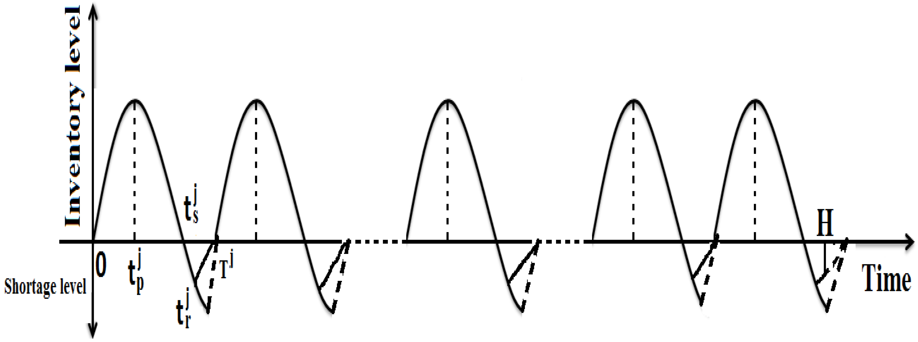
$t_p^j$	:	Time at which production stopped in each cycle
$t_s^j$	:	Time at which inventory exhausted in each cycle
$t_r^j$	:	Time at which production restarts in shortage period in each cycle
$T^j$	:	Length of each cycle
${\gamma }^j$	:	Portion of the demand that is not backlogged
$1-{\gamma }^j$	:	Portion of the demand that is backlogged
${\alpha }^j$	:	Achieved learning parameter to increase the rework rate
${\beta }^j$	:	Achieved learning parameter for production and screening costs
${\theta }^j$	:	Rate of breakability of the produced items
${\delta }^j$	:	Percentage of rework for breakable items related to the learning effect
$c_p^j$	:	Production cost per unit in the first cycle, $c_p^j{e}^{(i-1){\beta }^j}$ is the unit productioncost in $ith$ cycle
$c_{sr}^j$	:	Screening cost per unit in first cycle, $c_{sr}^j{e}^{(i-1){\beta }^j}$ is screening cost per unit in $ith$ cycle
$r_c^j$	:	Reworking cost per unit
$h_c^j$	:	Holding cost per unit per unit time for perfect quality items
$c_{sh}^j$	:	Shortage cost per unit per unit time for perfect quality items
$s^j$	:	Selling price per unit perfect quality items
R	:	Difference between inflation and the time value of money
$N^j$	:	Number of entirely accommodated cycles
M	:	Total number of items
H	:	Random time horizon length

2.2. Assumptions

The following assumptions are considered.

(i)

Non-perfect quality of multiple items is produced (breakable items) in the production system. A portion of breakable items is reworked to get a nearly perfect item. The perfect quality products are immediately set for sale.

(ii)

Demand rate ($D^j$) of $jth$ item ($j=1,2,\dots ,M$) is dependent on the displayed inventory level and selling price, which is of the form:

$$\begin{array}{c}\hfill D^j(q^j,s^j)=\left\{\begin{array}{cc}{d}_0^j+d_1^j{q}^j\left(t\right)-d_2^j{s}^j,\hfill & q^j\left(t\right)\ge 0\hfill \\ d_0^j-d_1^j{S}^j\left(t\right),\hfill & q^j\left(t\right)\le 0\hfill \end{array}\right.\end{array}$$

(1)

where $d_0^j$, $d_1^j$ and $d_2^j$ are positive constants.

(iii)

The time horizon H is not necessarily fixed and known. It has some uncertainty, therefore, it is finite and randomly distributed. Here, it is assumed that H follows an exponential distribution with the following probability density function (p.d.f)

$$\begin{array}{c}\hfill f\left(h\right)=\left\{\begin{array}{cc}\lambda e^{-\lambda h}\hfill & h\ge 0\hfill \\ 0\hfill & otherwise\hfill \end{array}\right.\end{array}$$

(2)

where $\lambda (>0)$ is the distribution parameter and h is the real value of H.

(iv)

First $N^j$ cycles are completely contained in the time horizon and it finishes during $(N^j+1)$th cycle.

(v)

Shortages are allowed in each cycle. After occurring shortage, some customers will wait in during the stockout period. So, it is considered the partial backlogging during the stockout period of unsatisfied market demand.

(vi)

The opening and terminal stock levels in each period are zero in each cycle.

(vii)

Due to fluctuation of the economy, the cost or price of every commodity is changed. For this reason, inflation and the time value of capital are considered.

(viii)

The learning experience of inspection process increases the rework rate of defective units and the amount of finished product. Learning effect influences the decision-maker to reduce more screening costs and rework costs to the next cycle.

3. Mathematical Formulation of the Production-Inventory Model

The on-hand stock diagram of the perfect quality items in the production-inventory model under the random planning horizon is shown in Figure 1. Screening and reworking of produced items continue with the production, the stock begins to accumulate constantly and at the same time jointly covering the demand with the rate of $D^j(q^j,s^j)$. Production, screening, and reworking of the items in the cycle stop at time $t_p^j$ and restart at time $t_r^j$, whereas inventory is exhausted at $t_s^j$ in the period of cycle $[(i-1)T^j,i{T}^j]$. In the fabrication process, both perfect and defective quality items are manufactured. The production process has a 100% screening through the manufacturing run time. The perfect quality products are ready for sale. Some defective quality products are continuously reworked during the production run time in order to restore their quality and to make them as perfect ones. The employees’ learning efforts increase the rate of reworking. In this regard, the amount of defective units is reduced thru manufacturing cycles.

3.1. Formulation for the $ith$ ($1\le i\le N^j$) Cycle for the $jth$ Item

Based on the description of the production-inventory model and Figure 1, the governing differential equations of the inventory level $q^j\left(t\right)$ for $ith$ ($1\le i\le N^j$) cycle are

$$\begin{array}{ccc}\hfill \frac{d{q}^j\left(t\right)}{dt}& =& \left\{\begin{array}{cc}(1-{\theta }^j)P^j+{\delta }^j{\left({\theta }^j{P}^j\right)}^{i{\alpha }^j}-D^j,\hfill & (i-1)T^j\le t\le (i-1)T^j+t_p^j\hfill \\ -D^j,\hfill & (i-1)T^j+t_p^j\le t\le (i-1)T^j+t_s^j\hfill \end{array}\right.\hfill \\ & =& \left\{\begin{array}{cc}(1-{\theta }^j)P^j+{\delta }^j{\left({\theta }^j{P}^j\right)}^{i{\alpha }^j}-\{d_0^j-d_2^j{s}^j+d_1^j{q}^j\left(t\right)\},\hfill & (i-1)T^j\le t\le (i-1)T^j+t_p^j\hfill \\ -\{d_0^j-d_2^j{s}^j+d_1^j{q}^j\left(t\right)\},\hfill & (i-1)T^j+t_p^j\le t\le (i-1)T^j+t_s^j\hfill \end{array}\right.\hfill \end{array}$$

where ${\delta }^j$ is the rework component of the imperfect portion ${\left({\theta }^j{P}^j\right)}^{i{\alpha }^j}$ in the $ith$ cycle, this increases thru of each cycle in concordance with the learning parameter ${\alpha }^j$.

The inventory level $q^j\left(t\right)$ during the period $[(i-1)T^j,(i-1)T^j+t_s^j]$ satisfies the conditions $q^j\left((i-1)T^j\right)=0$ and $q^j((i-1)T^j+t_s^j)=0$.

The solution of the differential equations is given below

$$\begin{array}{c}\hfill q^j\left(t\right)=\left\{\begin{array}{c}\frac{1}{d_1^j}\left\{(1-{\theta }^j)P^j+{\delta }^j{\left({\theta }^j{P}^j\right)}^{i{\alpha }^j}-(d_0^j-d_2^j{s}^j)\right\}\hfill \\ \times \left[1-e^{-d_1^j\{t-(i-1)T^j\}}\right],\hfill & (i-1)T^j\le t\le (i-1)T^j+t_p^j\hfill \\ -\frac{(d_0^j-d_2^j{s}^j)}{d_1^j}\left[1-e^{-d_1^j\{t-(i-1)T^j-t_s^j\}}\right],\hfill & (i-1)T^j+t_p^j\le t\le (i-1)T^j+t_s^j\hfill \end{array}\right.\end{array}$$

(3)

During the period $[(i-1)T^j+t_s^j,i{T}^j]$, the demand rate is $D^j\left(S^j\right)=\{d_0^j-d_2^j{s}^j-d_1^j{S}^j\left(t\right)\}$. This time is the shortage period. Consequently, the shortage level $S^j\left(t\right)$ is regulated by the following differential equation:

$$\begin{array}{c}\hfill \frac{d{S}^j\left(t\right)}{dt}=\left\{\begin{array}{cc}\{d_0^j-d_1^j{S}^j\left(t\right)\},\hfill & [(i-1)T^j+t_s^j,(i-1)T^j+t_r^j]\hfill \\ (1-{\theta }^j)P^j+{\delta }^j{\left({\theta }^j{P}^j\right)}^{i{\alpha }^j}-(d_0^j-d_2^j{s}^j),\hfill & [(i-1)T^j+t_r^j,i{T}^j]\hfill \end{array}\right.\end{array}$$

subject to the following conditions: $S^j((i-1)T^j+t_s^j)=0$ and $S^j\left(i{T}^j\right)=0$.

The solution of the differential equations is expressed as follows:

$$\begin{array}{c}\hfill S^j\left(t\right)=\left\{\begin{array}{cc}\frac{d_0^j}{d_1^j}\left[1-e^{-d_1^j\{t-(i-1)T^j-t_s^j\}}\right],\hfill & [(i-1)T^j+t_s^j,(i-1)T^j+t_r^j]\hfill \\ \left\{(1-{\theta }^j)P^j+{\delta }^j{\left({\theta }^j{P}^j\right)}^{i{\alpha }^j}-(d_0^j-d_2^j{s}^j)\right\}(t-i{T}^j),\hfill & [(i-1)T^j+t_r^j,i{T}^j]\hfill \end{array}\right.\end{array}$$

The maximum shortage amount ($S^j$) of $jth$ item is

$$\begin{array}{c}\hfill S^j=S^j((i-1)T^j+t_r^j)=\frac{d_0^j}{d_1^j}\left\{1-e^{-d_1^j(t_r^j-t_s^j)}\right\}\end{array}$$

The holding cost for the $ith$ cycle is represented by

$$\begin{array}{ccc}\hfill H{C}_i^j& =& h_c^j\left[{\int }_{(i-1)T^j}^{(i-1)T^j+t_s^j}{q}^j\left(t\right)e^{-Rt}dt\right]\hfill \\ & =& h_c^j\left[{\int }_{(i-1)T^j}^{(i-1)T^j+t_p^j}{q}^j\left(t\right)e^{-Rt}dt+{\int }_{(i-1)T^j+t_p^j}^{(i-1)T^j+t_s^j}{q}^j\left(t\right)e^{-Rt}dt\right]\hfill \\ & =& \frac{h_c^j}{d_1^j}\left\{(1-{\theta }^j)P^j+{\delta }^j{\left({\theta }^j{P}^j\right)}^{i{\alpha }^j}-(d_0^j-d_2^j{s}^j)\right\}\left[\frac{1-e^{-R{t}_p^j}}{R}-\frac{1-e^{-(R+d_1^j)t_p^j}}{R+d_1^j}\right]e^{-(i-1)R{T}^j}\hfill \\ & & -\frac{h_c^j(d_0^j-d_2^j{s}^j)}{d_1^j}\left[\frac{1}{R}(e^{-R{t}_p^j}-e^{-R{t}_s^j})-\frac{e^{d_1^j{t}_s^j}}{R+d_1^j}\{e^{-(R+d_1^j)t_p^j}-e^{-(R+d_1^j)t_s^j}\}\right]e^{-R(i-1)T^j}\hfill \end{array}$$

The production cost of the $ith$ cycle is given as follows:

$$\begin{array}{ccc}\hfill P{C}_i^j& =& c_p^j{e}^{(i-1){\beta }^j}\left[{\int }_{(i-1)T^j}^{(i-1)T^j+t_p^j}{P}^j{e}^{-Rt}dt+{\int }_{(i-1)T^j+t_r^j}^{i{T}^j}{P}^j{e}^{-Rt}dt\right]\hfill \\ & =& \frac{c_p^j}{R}{P}^j\left[(1-e^{-R{t}_p^j})+(e^{-R{t}_r^j}-e^{-R{T}^j})\right]e^{-(i-1)(R{T}^j-{\beta }^j)}\hfill \end{array}$$

The term $e^{(i-1){\beta }^j}$ decreases the production cost for the next cycle due to the increasing of the learning rate ${\beta }^j$. The term $e^{-Rt}$ takes into consideration the effect of the inflation rate R on the production cost.

The screening cost of the $ith$ cycle is computed with

$$\begin{array}{ccc}\hfill S{C}_i^j& =& c_{sr}^j{e}^{(i-1){\beta }^j}\left[{\int }_{(i-1)T^j}^{(i-1)T^j+t_p^j}{P}^j{e}^{-Rt}dt+{\int }_{(i-1)T^j+t_r^j}^{i{T}^j}{P}^j{e}^{-Rt}dt\right]\hfill \\ & =& \frac{c_{sr}^j}{R}{P}^j\left[(1-e^{-R{t}_p^j})+(e^{-R{t}_r^j}-e^{-R{T}^j})\right]e^{-(i-1)(R{T}^j-{\beta }^j)}\hfill \end{array}$$

The reworking cost of the $ith$ cycle is calculated as follows:

$$\begin{array}{ccc}\hfill R{C}_i^j& =& r_c^j\left[{\int }_{(i-1)T^j}^{(i-1)T^j+t_p^j}{\delta }^j{\left({\theta }^j{P}^j\right)}^{i{\alpha }^j}{e}^{-Rt}dt+{\int }_{(i-1)T^j+t_r^j}^{i{T}^j}{\delta }^j{\left({\theta }^j{P}^j\right)}^{i{\alpha }^j}{e}^{-Rt}dt\right]\hfill \\ & =& \frac{1}{R}{r}_c^j{\delta }^j{\left({\theta }^j{P}^j\right)}^{i{\alpha }^j}\left[(1-e^{-R{t}_p^j})+(e^{-R{t}_r^j}-e^{-R{T}^j})\right]e^{-R(i-1)T^j}\hfill \end{array}$$

The shortage cost of the $ith$ period is determined with

$$\begin{array}{ccc}\hfill S{H}_i^j& =& c_{sh}^j(1-{\gamma }^j){\int }_{(i-1)T^j+t_s^j}^{(i-1)T^j+t_r^j}{S}^j\left(t\right)e^{-Rt}dt\hfill \\ & =& c_{sh}^j(1-{\gamma }^j)\frac{d_0^j}{d_1^j}\left[\frac{1}{R}(e^{-R{t}_s^j}-e^{-R{t}_r^j})-\frac{e^{d_1^j{t}_s^j}}{R+d_1^j}\{e^{-(R+d_1^j)t_s^j}-e^{-(R+d_1^j)t_r^j}\}\right]e^{-R(i-1)T^j}\hfill \end{array}$$

The whole cost of the production-inventory model for the first $N^j$ fully accommodated periods is given as follows

$$\begin{array}{ccc}\hfill T{C}^j\left(P^j\right)& =& \sum _{i=1}^{N^j}\left[P{C}_i^j+S{C}_i^j+R{C}_i^j+H{C}_i^j+S{H}_i^j\right]\hfill \\ & =& \frac{P^j}{R}(c_p^j+c_{sr}^j)\left\{(1-e^{-R{t}_p^j})+(e^{-R{t}_r^j}-e^{-R{T}^j})\right\}\frac{1-e^{-N^j(R{T}^j-{\beta }^j)}}{1-e^{-R{T}^j}}\hfill \\ & +& {\delta }^j{\left({\theta }^j{P}^j\right)}^{{\alpha }^j}[\frac{r_c^j}{R}\left\{(1-e^{-R{t}_p^j})+(e^{-R{t}_r^j}-e^{-R{T}^j})\right\}\hfill \\ & +& \frac{h_c^j}{d_1^j}\left\{\frac{1-e^{-R{t}_p^j}}{R}-\frac{1-e^{-(R+d_1^j)t_p^j}}{R+d_1^j}\right\}]\frac{1-{\left\{e^{-R{T}^j}{\left({\theta }^j{P}^j\right)}^{{\alpha }^j}\right\}}^{N^j}}{1-\left\{e^{-R{T}^j}{\left({\theta }^j{P}^j\right)}^{{\alpha }^j}\right\}}\hfill \\ & +& \frac{h_c^j}{d_1^j}[\left\{(1-{\theta }^j)P^j-(d_0^j-d_2^j{s}^j)\right\}\left\{\frac{1-e^{-R{t}_p^j}}{R}-\frac{1-e^{-(R+d_1^j)t_p^j}}{R+d_1^j}\right\}\hfill \\ & -& (d_0^j-d_2^j{s}^j)\left\{\frac{1}{R}(e^{-R{t}_p^j}-e^{-R{t}_s^j})-\frac{e^{d_1^j{t}_s^j}}{R+d_1^j}\{e^{-(R+d_1^j)t_p^j}-e^{-(R+d_1^j)t_s^j}\}\right\}]\frac{1-e^{-N^{j}R{T}^j}}{1-e^{-R{T}^j}}\hfill \\ & +& c_{sh}^j(1-{\gamma }^j)\frac{d_0^j}{d_1^j}\left[\frac{1}{R}(e^{-R{t}_s^j}-e^{-R{t}_r^j})-\frac{e^{d_1^j{t}_s^j}}{R+d_1^j}\{e^{-(R+d_1^j)t_s^j}-e^{-(R+d_1^j)t_r^j}\}\right]\frac{1-e^{-N^{j}R{T}^j}}{1-e^{-R{T}^j}}\hfill \end{array}$$

Because of the $f\left(h\right)$ is the p.d.f of the time horizon H, consequently, the expected total cost from the $N^j$ completed cycles is given as follows,

$$\begin{array}{ccc}\hfill E\left[TC\left(P^j\right)\right]& =& \sum _{N^j=0}^{\infty }{\int }_{N^j{T}^j}^{(N^j+1)T^j}TC(t_p^j,T^j)f\left(h\right)dh\hfill \\ & =& \frac{1}{R}\left\{(1-e^{-R{t}_p^j})+(e^{-R{t}_r^j}-e^{-R{T}^j})\right\}[\frac{r_c^j(1-{\theta }^j)P^j{e}^{-\lambda T^j}}{\{1-e^{-(\lambda +R)T^j}\}}\hfill \\ & & +\frac{P^j(c_p^j+c_{sr}^j)e^{-\lambda T^j}\{1-e^{-(R{T}^j-{\beta }^j)}\}}{\left(1-e^{-R{T}^j}\right)\{1-e^{-(\lambda T^j+R{T}^j-{\beta }^j)}\}}]\hfill \\ & +& \frac{h_c^j}{d_1^j}{\delta }^j{\left({\theta }^j{P}^j\right)}^{{\alpha }^j}\left\{\frac{1-e^{-R{t}_p^j}}{R}-\frac{1-e^{-(R+d_1^j)t_p^j}}{R+d_1^j}\right\}\frac{e^{-\lambda T^j}}{1-{\left({\theta }^j{P}^j\right)}^{{\alpha }^j}{e}^{-(\lambda +R)T^j}}\hfill \\ & +& \frac{h_c^j{e}^{-\lambda T^j}}{d_1^j\{1-e^{-(\lambda +R)T^j}\}}[\left\{(1-{\theta }^j)P^j-(d_0^j-d_2^j{s}^j)\right\}\left\{\frac{1-e^{-R{t}_p^j}}{R}-\frac{1-e^{-(R+d_1^j)t_p^j}}{R+d_1^j}\right\}\hfill \\ & -& (d_0^j-d_2^j{s}^j)\left\{\frac{1}{R}(e^{-R{t}_p^j}-e^{-R{t}_s^j})-\frac{e^{d_1^j{t}_s^j}}{R+d_1^j}\{e^{-(R+d_1^j)t_p^j}-e^{-(R+d_1^j)t_s^j}\}\right\}]\hfill \\ & +& \frac{d_0^j{c}_{sh}^j(1-{\gamma }^j)e^{-\lambda T^j}}{d_1^j\{1-e^{-(\lambda +R)T^j}\}}\left[\frac{1}{R}(e^{-R{t}_s^j}-e^{-R{t}_r^j})-\frac{e^{d_1^j{t}_s^j}}{R+d_1^j}\{e^{-(R+d_1^j)t_s^j}-e^{-(R+d_1^j)t_r^j}\}\right]\hfill \end{array}$$

3.2. Formulation for the Last Cycle for the $jth$ Item

The time horizon H is random, so the previous cycle of the production-inventory model ends with four mutually exclusive cases. In each case, the stock level $\left(q_L^j\left(t\right)\right)$ in the period length $[N^j{T}^j,(N^j+1)T^j]$ is supported by the following differential equations.

$$\begin{array}{ccc}\hfill \frac{d{q}_L^j\left(t\right)}{dt}& =& \left\{\begin{array}{cc}(1-{\theta }^j)P^j+{\delta }^j{\left({\theta }^j{P}^j\right)}^{(N^j+1){\alpha }^j}-\{d_0^j+d_1^j{q}^j\left(t\right)-d_2^j{s}^j\},\hfill & N^j{T}^j\le t\le N^j{T}^j+t_p^j\hfill \\ -\{d_0^j+d_1^j{q}^j\left(t\right)-d_2^j{s}^j\},\hfill & N^j{T}^j+t_p^j\le t\le N^j{T}^j+t_s^j\hfill \end{array}\right.\hfill \end{array}$$

subject to the conditions $q_L^j\left(N^j{T}^j\right)=0$ and $q_L^j(N^j{T}^j+t_s^j)=0$.

The solution of this differential equations is given below

$$\begin{array}{c}\hfill q_L^j\left(t\right)=\left\{\begin{array}{c}\frac{1}{d_1^j}\{(1-{\theta }^j)P^j+{\delta }^j{\left({\theta }^j{P}^j\right)}^{(N^j+1){\alpha }^j}\hfill \\ -(d_0^j-d_2^j{s}^j)\}\left[1-e^{-d_1^j\{t-N^j{T}^j\}}\right],\hfill & N^j{T}^j\le t\le N^j{T}^j+t_p^j\hfill \\ -\frac{(d_0^j-d_2^j{s}^j)}{d_1^j}\left[1-e^{-d_1^j\{t-N^j{T}^j-t_s^j\}}\right],\hfill & N^j{T}^j+t_p^j\le t\le N^j{T}^j+t_s^j\hfill \end{array}\right.\end{array}$$

(4)

During the period $[(N^j{T}^j+t_s^j,(N^j+1)T^j]$, the demand rate is $D^j=(d_0^j-d_2^j{s}^j)-d_1^j{S}^j\left(t\right)$ and this interval corresponds to the shortage period. Therefore, the shortage level $S_L^j\left(t\right)$ is ruled by the differential equation as follows:

$$\begin{array}{c}\hfill \frac{d{S}_L^j\left(t\right)}{dt}=\left\{\begin{array}{cc}\{d_0^j-d_1^j{S}^j\left(t\right)\},\hfill & [N^j{T}^j+t_s^j,N^j{T}^j+t_r^j]\hfill \\ (1-{\theta }^j)P^j+{\delta }^j{\left({\theta }^j{P}^j\right)}^{(N^j+1){\alpha }^j}-(d_0^j-d_2^j{s}^j),\hfill & [N^j{T}^j+t_r^j,(N^j+1)T^j]\hfill \end{array}\right.\end{array}$$

subject to the following condition $S_L^j(N^j{T}^j+t_s^j)=0$.

The solution of the differential equations is

$$\begin{array}{c}\hfill S_L^j\left(t\right)=\left\{\begin{array}{cc}\frac{d_0^j}{d_1^j}\left[1-e^{-d_1^j\{t-N^j{T}^j-t_s^j\}}\right],\hfill & [N^j{T}^j+t_s^j,N^j{T}^j+t_r^j]\hfill \\ \left\{(1-{\theta }^j)P^j+{\delta }^j{\left({\theta }^j{P}^j\right)}^{(N^j+1){\alpha }^j}-(d_0^j-d_2^j{s}^j)\right\}(t-i{T}^j),\hfill & [N^j{T}^j+t_r^j,(N^j+1)T^j]\hfill \end{array}\right.\end{array}$$

In the last cycle, four cases are considered depending only upon the period size. Let, h be the value related to the random variable H.

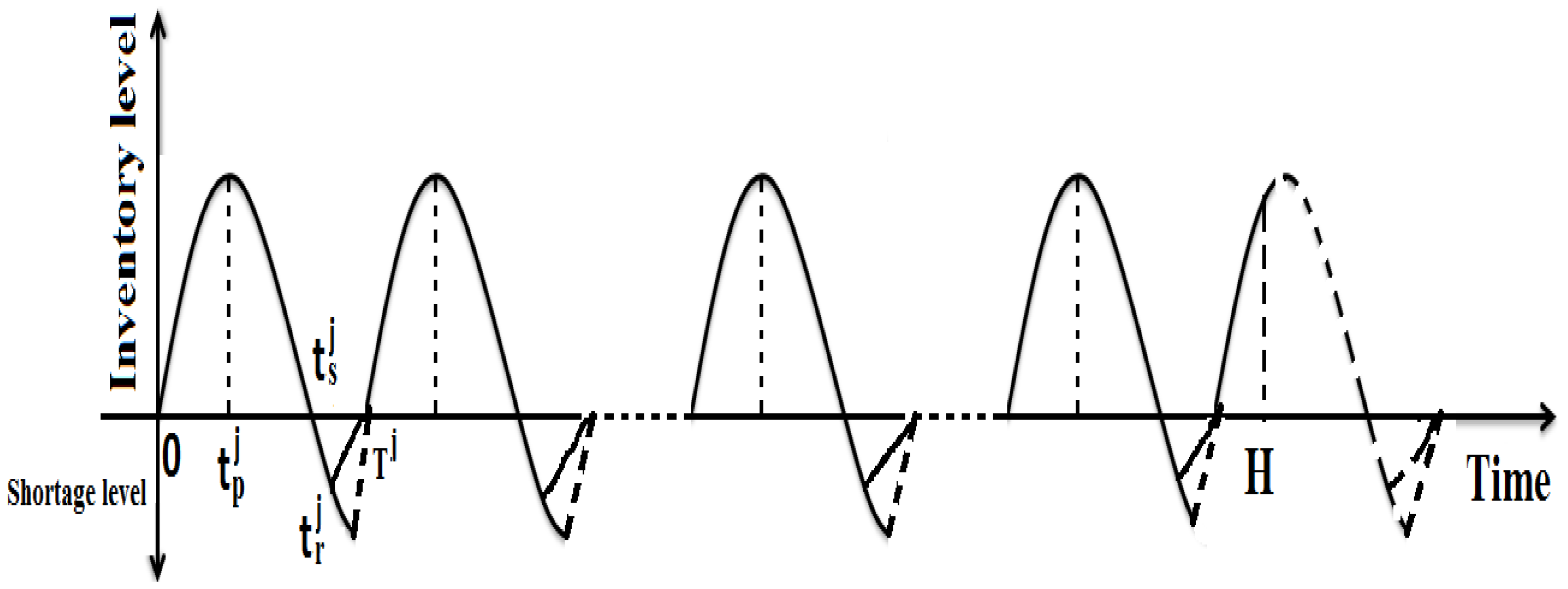
3.2.1. Case-I ($N^j{T}^j\le h\le N^j{T}^j+t_p^j$)

In this case, the business period is completed at any point of the production run time of the last cycle as it is shown in Figure 2.

The production cost of the last cycle is obtained with the following mathematical expression,

$$\begin{array}{ccc}\hfill P{C}_{L_1}^j& =& c_p^j{e}^{N^j{\beta }^j}\left[{\int }_{N^j{T}^j}^h{P}^j{e}^{-Rt}dt\right]=\frac{c_p^j}{R}{P}^j{e}^{N^j{\beta }^j}(e^{-R{N}^j{T}^j}-e^{-Rh})\hfill \end{array}$$

The screening cost of the last cycle is formulated as,

$$\begin{array}{ccc}\hfill S{C}_{L_1}^j& =& c_{sr}^j{e}^{N^j{\beta }^j}\left[{\int }_{N^j{T}^j}^h{P}^j{e}^{-Rt}dt\right]=\frac{c_{sr}^j}{R}{P}^j{e}^{N^j{\beta }^j}(e^{-R{N}^j{T}^j}-e^{-Rh})\hfill \end{array}$$

The reworking cost of the last cycle is described as,

$$\begin{array}{ccc}\hfill R{C}_{L_1}^j& =& r_c^j{\int }_{N^j{T}^j}^h{\delta }^j{\left({\theta }^j{P}^j\right)}^{(N^j+1){\alpha }^j}{e}^{-Rt}dt=\frac{r_c^j}{R}{\delta }^j{\left({\theta }^j{P}^j\right)}^{(N^j+1){\alpha }^j}\left\{e^{-R{N}^j{T}^j}-e^{-Rh}\right\}\hfill \end{array}$$

The holding cost of the last cycle is determined with,

$$\begin{array}{ccc}\hfill H{C}_{L_1}^j& =& h_c^j\left[{\int }_{N^j{T}^j}^h{q}_L^j\left(t\right)e^{-Rt}dt\right]\hfill \\ & =& \frac{h_c^j}{d_1^j}\left\{(1-{\theta }^j)P^j+{\delta }^j{\left({\theta }^j{P}^j\right)}^{(N^j+1){\alpha }^j}-(d_0^j-d_2^j{s}^j)\right\}{\int }_{N^j{T}^j}^h\left\{1-e^{-d_1^j(t-N^j{T}^j)}\right\}{e}^{-Rt}dt\hfill \\ & =& \frac{h_c^j}{d_1^j}\left\{(1-{\theta }^j)P^j+{\delta }^j{\left({\theta }^j{P}^j\right)}^{(N^j+1){\alpha }^j}-(d_0^j-d_2^j{s}^j)\right\}[\frac{1}{R}(e^{-R{N}^j{T}^j}-e^{-Rh})\hfill \\ & -& \frac{e^{d_1^j{N}^j{T}^j}}{R+d_1^j}\left\{e^{-(d_1^j+R)N^j{T}^j}-e^{-(d_1^j+R)h}\right\}]\hfill \end{array}$$

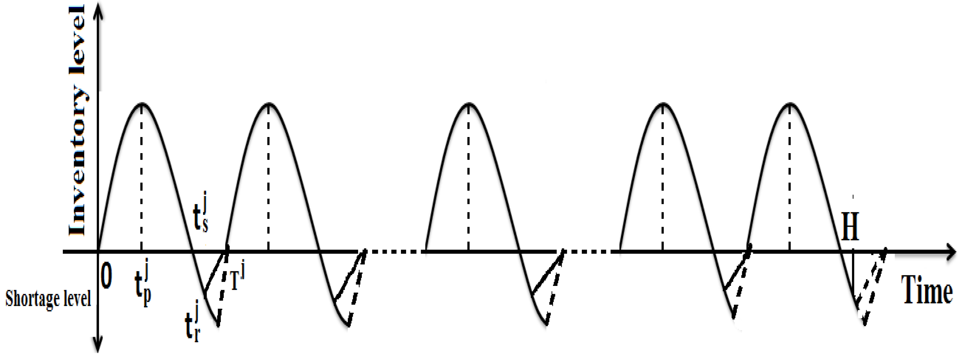
3.2.2. Case-II ($N^j{T}^j+t_p^j\le h\le N^j{T}^j+t_s^j$)

In this case, the business period is completed after production run time but before shortage period which is shown by Figure 3.

The production cost of the last cycle is calculated as follows,

$$\begin{array}{ccc}\hfill P{C}_{L_2}^j& =& c_p^j{e}^{N^j{\beta }^j}{\int }_{N^j{T}^j}^{N^j{T}^j+t_p^j}{P}^j{e}^{-Rt}dt=\frac{c_p^j}{R}{P}^j(1-e^{-R{t}_p^j})e^{-(R{T}^j-{\beta }^j)N^j}\hfill \end{array}$$

The screening cost of the last cycle is formulated as,

$$\begin{array}{ccc}\hfill S{C}_{L_2}^j& =& c_{sr}^j{e}^{N^j{\beta }^j}{\int }_{N^j{T}^j}^{N^j{T}^j+t_p^j}{P}^j{e}^{-Rt}dt=\frac{c_{sr}^j}{R}{P}^j(1-e^{-R{t}_p^j})e^{-(R{T}^j-{\beta }^j)N^j}\hfill \end{array}$$

The reworking cost of the last cycle is determined with,

$$\begin{array}{ccc}\hfill R{C}_{L_2}^j& =& r_c^j{\int }_{N^j{T}^j}^{N^j{T}^j+t_p^j}{\delta }^j{\left({\theta }^j{P}^j\right)}^{(N^j+1){\alpha }^j}{e}^{-Rt}dt=\frac{r_c^j}{R}{\delta }^j{\left({\theta }^j{P}^j\right)}^{(N^j+1){\alpha }^j}(1-e^{-R{t}_p^j})e^{-R{N}^j{T}^j}\hfill \end{array}$$

The holding cost of the last cycle is computed with,

$$\begin{array}{ccc}\hfill H{C}_{L_2}^j& =& h_c^j\left[{\int }_{N^j{T}^j}^{N^j{T}^j+t_p^j}{q}_L^j\left(t\right)e^{-Rt}dt+{\int }_{N^j{T}^j+t_p^j}^h{q}_L^j\left(t\right)e^{-Rt}dt\right]\hfill \\ & =& \frac{h_c^j}{d_1^j}\left\{(1-{\theta }^j)P^j+{\delta }^j{\left({\theta }^j{P}^j\right)}^{(N^j+1){\alpha }^j}\right\}\left[\frac{1}{R}\left(1-e^{-R{t}_p^j}\right)-\frac{1}{R+d_1^j}\left\{1-e^{-(R+d_1^j)t_p^j}\right\}\right]e^{-R{N}^j{T}^j}\hfill \\ & +& \frac{h_c^j}{d_1^j}(d_0^j-d_2^j{s}^j)\left[\frac{e^{-R{N}^j{T}^j}}{R+d_1^j}\left\{1-e^{-(R+d_1^j)t_p^j}\right\}+\frac{e^{d_1^j(N^j{T}^j+t_s^j)}}{R+d_1^j}\left\{e^{-(R+d_1^j)(N^j{T}^j+t_p^j)}-e^{-(R+d_1^j)h}\right\}\right]\hfill \\ & -& \frac{h_c^j}{d_1^{j}R}(d_0^j-d_2^j{s}^j)\left(e^{-R{N}^j{T}^j}-e^{-Rh}\right)\hfill \end{array}$$

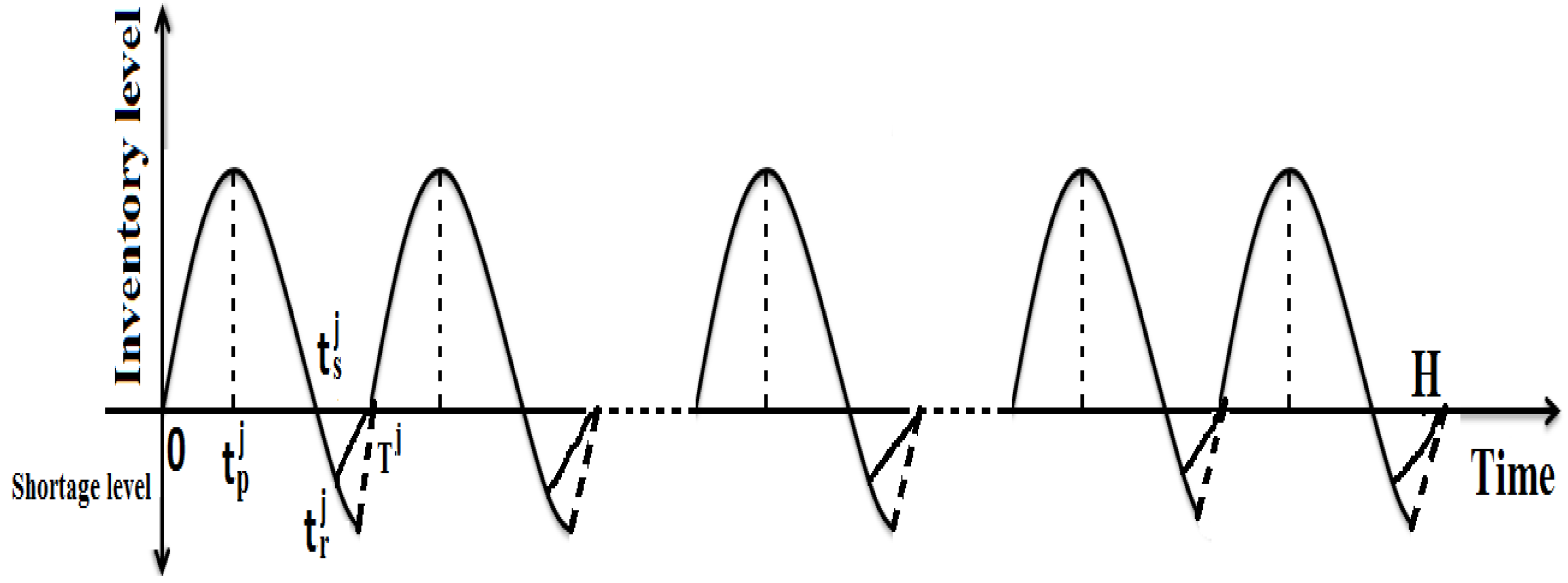
3.2.3. Case-III ($N^j{T}^j+t_s^j\le h\le N^j{T}^j+t_r^j$)

In this case, the business period is completed at any point of the shortage period ($N^j{T}^j+t_s^j\le h\le N^j{T}^j+t_r^j$) which is shown by Figure 4.

The production cost of the last cycle is described by,

$$\begin{array}{ccc}\hfill P{C}_{L_3}^j& =& c_p^j{e}^{N^j{\beta }^j}{\int }_{N^j{T}^j}^{N^j{T}^j+t_p^j}{P}^j{e}^{-Rt}dt=\frac{c_p^j}{R}{P}^j(1-e^{-R{t}_p^j})e^{-(R{T}^j-{\beta }^j)N^j}\hfill \end{array}$$

The screening cost of the last cycle is formulated as,

$$\begin{array}{ccc}\hfill S{C}_{L_3}^j& =& c_{sr}^j{e}^{N^j{\beta }^j}{\int }_{N^j{T}^j}^{N^j{T}^j+t_p^j}{P}^j{e}^{-Rt}dt=\frac{c_{sr}^j}{R}{P}^j(1-e^{-R{t}_p^j})e^{-(R{T}^j-{\beta }^j)N^j}\hfill \end{array}$$

The reworking cost of the last cycle is given below,

$$\begin{array}{ccc}\hfill R{C}_{L_3}^j& =& r_c^j{\int }_{N^j{T}^j}^{N^j{T}^j+t_p^j}{\delta }^j{\left({\theta }^j{P}^j\right)}^{(N^j+1){\alpha }^j}{e}^{-Rt}dt=\frac{r_c^j}{R}{\delta }^j{\left({\theta }^j{P}^j\right)}^{(N^j+1){\alpha }^j}(1-e^{-R{t}_p^j})e^{-R{N}^j{T}^j}\hfill \end{array}$$

The holding cost of the last cycle is obtained by following mathematical expression,

$$\begin{array}{ccc}\hfill H{C}_{L_3}^j& =& h_c^j\left[{\int }_{N^j{T}^j}^{N^j{T}^j+t_p^j}{q}^j\left(t\right)e^{-Rt}dt+{\int }_{N^j{T}^j+t_p^j}^{N^j{T}^j+t_s^j}{q}^j\left(t\right)e^{-Rt}dt\right]\hfill \\ & =& \frac{h_c^j}{d_1^j}\left\{(1-{\theta }^j)P^j+{\delta }^j{\left({\theta }^j{P}^j\right)}^{(N^j+1){\alpha }^j}\right\}\left[\frac{1}{R}\left(1-e^{-R{t}_p^j}\right)-\frac{1}{R+d_1^j}\left\{1-e^{-(R+d_1^j)t_p^j}\right\}\right]e^{-R{N}^j{T}^j}\hfill \\ & +& \frac{h_c^j}{d_1^j}(d_0^j-d_2^j{s}^j)[\frac{e^{-R{N}^j{T}^j}}{R+d_1^j}\left\{1-e^{-(R+d_1^j)t_p^j}\right\}+\frac{e^{d_1^j(N^j{T}^j+t_s^j)}}{R+d_1^j}\{e^{-(R+d_1^j)(N^j{T}^j+t_p^j)}\hfill \\ & -& e^{-(R+d_1^j)\left(N^j{T}^j+t_s^j\right)}\left\}\right]-\frac{h_c^j}{d_1^{j}R}(d_0^j-d_2^j{s}^j)\left(e^{-R{N}^j{T}^j}-e^{-R\left(N^j{T}^j+t_s^j\right)}\right)\hfill \end{array}$$

The shortage cost of the last cycle is formulated by

$$\begin{array}{ccc}\hfill S{H}_3^j& =& c_{sh}^j{\int }_{N^j{T}^j+t_s^j}^h{S}_L^j\left(t\right)e^{-Rt}dt\hfill \\ & =& c_{sh}^j{\int }_{N^j{T}^j+t_s^j}^h\frac{d_0^j}{d_1^j}\left\{1-e^{-d_1^j(t-N^j{T}^j-t_s^j)}\right\}{e}^{-Rt}dt\hfill \\ & =& c_{sh}^j\frac{d_0^j}{d_1^j}\left[\frac{1}{R}\left\{e^{-R(N^j{T}^j+t_s^j)}-e^{-Rh}\right\}-\frac{e^{d_1^j(N^j{T}^j+t_s^j)}}{R+d_1^j}\left\{e^{-(R+d_1^j)(N^j{T}^j+t_s^j)}-e^{-(R+d_1^j)h}\right\}\right]\hfill \end{array}$$

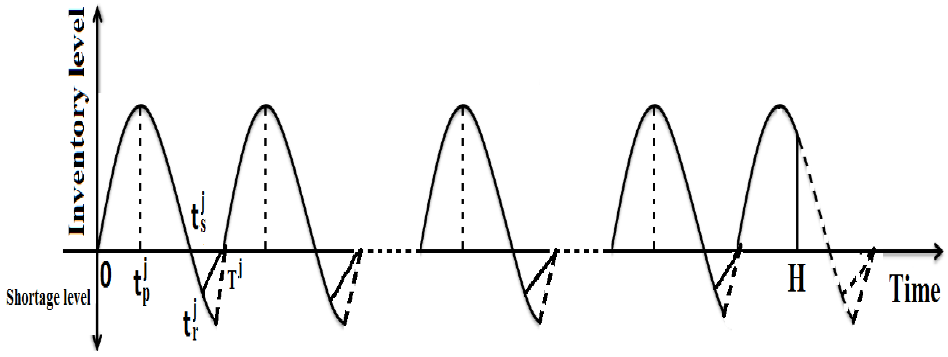
3.2.4. Case-IV ($N^j{T}^j+t_r^j\le h\le (N^j+1)T^j$)

In this case, the business period is completed in the shortage period ($N^j{T}^j+t_r^j\le h\le (N^j+1)T^j$) which is shown by Figure 5.

The production cost of the last cycle is determined with,

$$\begin{array}{ccc}\hfill P{C}_{L_4}^j& =& c_p^j{e}^{N^j{\beta }^j}\left[{\int }_{N^j{T}^j}^{N^j{T}^j+t_p^j}{P}^j{e}^{-Rt}dt+{\int }_{N^j{T}^j+t_r^j}^h{P}^j{e}^{-Rt}dt\right]\hfill \\ & =& \frac{c_p^j}{R}{P}^j\left[(1-e^{-R{t}_p^j}+e^{-R{t}_r^j})e^{-(R{T}^j-{\beta }^j)N^j}-e^{N^j{\beta }^j}{e}^{-Rh}\right]\hfill \end{array}$$

The screening cost of the last cycle is formulated as,

$$\begin{array}{ccc}\hfill S{C}_{L_4}^j& =& c_{sr}^j{e}^{N^j{\beta }^j}\left[{\int }_{N^j{T}^j}^{N^j{T}^j+t_p^j}{P}^j{e}^{-Rt}dt+{\int }_{N^j{T}^j+t_r^j}^h{P}^j{e}^{-Rt}dt\right]\hfill \\ & =& \frac{c_{sr}^j}{R}{P}^j\left[(1-e^{-R{t}_p^j}+e^{-R{t}_r^j})e^{-(R{T}^j-{\beta }^j)N^j}-e^{N^j{\beta }^j}{e}^{-Rh}\right]\hfill \end{array}$$

The reworking cost of the last cycle is computed as follows,

$$\begin{array}{ccc}\hfill R{C}_{L_4}^j& =& r_c^j\left[{\int }_{N^j{T}^j}^{N^j{T}^j+t_p^j}{\delta }^j{\left({\theta }^j{P}^j\right)}^{(N^j+1){\alpha }^j}{e}^{-Rt}dt+{\int }_{N^j{T}^j+t_r^j}^h{\delta }^j{\left({\theta }^j{P}^j\right)}^{(N^j+1){\alpha }^j}{e}^{-Rt}dt\right]\hfill \\ & =& \frac{r_c^j}{R}{\delta }^j{\left({\theta }^j{P}^j\right)}^{(N^j+1){\alpha }^j}\left[(1-e^{-R{t}_p^j}+e^{-R{t}_r^j})e^{-R{N}^j{T}^j}-e^{-Rh}\right]\hfill \end{array}$$

The holding cost of the last cycle is calculated by the following expression

$$\begin{array}{ccc}\hfill H{C}_{L_4}^j& =& h_c^j\left[{\int }_{N^j{T}^j}^{N^j{T}^j+t_p^j}{q}_L^j\left(t\right)e^{-Rt}dt+{\int }_{N^j{T}^j+t_p^j}^{N^j{T}^j+t_s^j}{q}_L^j\left(t\right)e^{-Rt}dt\right]\hfill \\ & =& \frac{h_c^j}{d_1^j}\left\{(1-{\theta }^j)P^j+{\delta }^j{\left({\theta }^j{P}^j\right)}^{(N^j+1){\alpha }^j}\right\}\left[\frac{1}{R}\left(1-e^{-R{t}_p^j}\right)-\frac{1}{R+d_1^j}\left\{1-e^{-(R+d_1^j)t_p^j}\right\}\right]e^{-R{N}^j{T}^j}\hfill \\ & +& \frac{h_c^j}{d_1^j}(d_0^j-d_2^j{s}^j)\left[\frac{e^{-R{N}^j{T}^j}}{R+d_1^j}\left\{1-e^{-(R+d_1^j)t_p^j}\right\}+\frac{e^{d_1^j(N^j{T}^j+t_s^j)}}{R+d_1^j}\left\{e^{-(R+d_1^j)(N^j{T}^j+t_p^j)}-e^{-(R+d_1^j)\left(N^j{T}^j+t_s^j\right)}\right\}\right]\hfill \\ & -& \frac{h_c^j}{d_1^{j}R}(d_0^j-d_2^j{s}^j)\left(e^{-R{N}^j{T}^j}-e^{-R\left(N^j{T}^j+t_s^j\right)}\right)\hfill \end{array}$$

The shortage cost of the last cycle is formulated by

$$\begin{array}{ccc}\hfill S{H}_{L_4}^j& =& c_{sh}^j(1-{\gamma }^j){\int }_{N^j{T}^j+t_s^j}^{N^j{T}^j+t_r^j}{S}^j\left(t\right)e^{-Rt}dt\hfill \\ & =& c_{sh}^j(1-{\gamma }^j){\int }_{N^j{T}^j+t_s^j}^{N^j{T}^j+t_r^j}\frac{d_0^j}{d_1^j}\left\{1-e^{-d_1^j(t-N^j{T}^j-t_s^j)}\right\}{e}^{-Rt}dt\hfill \\ & =& c_{sh}^j(1-{\gamma }^j)\frac{d_0^j}{d_1^j}\left[\frac{1}{R}\left\{e^{-R{t}_s^j}-e^{-R{t}_r^j}\right\}-\frac{e^{d_1^j{t}_s^j}}{R+d_1^j}\left\{e^{-(R+d_1^j)t_s^j}-e^{-(R+d_1^j)t_r^j}\right\}\right]e^{-R{N}^j{T}^j}\hfill \end{array}$$

The expected production cost of the last cycle is determined by,

$$\begin{array}{ccc}\hfill E\left[P{C}_L^j\right]& =& \sum _{N^j=0}^{\infty }[{\int }_{N^j{T}^j}^{N^j{T}^j+t_p^j}P{C}_{L_1}^{j}f\left(h\right)dh+{\int }_{N^j{T}^j+t_p^j}^{N^j{T}^j+t_s^j}P{C}_{L_2}^{j}f\left(h\right)dh\hfill \\ & +& {\int }_{N^j{T}^j+t_s^j}^{N^j{T}^j+t_r^j}P{C}_{L_3}^{j}f\left(h\right)dh+{\int }_{N^j{T}^j+t_r^j}^{(N^j+1)T^j}P{C}_{L_4}^{j}f\left(h\right)dh]\hfill \\ & =& \frac{c_p^j{P}^j}{R\{1-e^{-\{\left(R+\lambda \right)T^j-{\beta }^j\}}\}}[\frac{R}{R+\lambda }\left\{1-e^{-\left(R+\lambda \right)t_p^j}+e^{-\left(R+\lambda \right)t_r^j}\right\}\hfill \\ & -& e^{-\lambda T^j}\left\{1-e^{-R{t}_p^j}+e^{-R{t}_r^j}\right\}+\frac{\lambda }{R+\lambda }{e}^{-\left(R+\lambda \right)T^j}]\hfill \end{array}$$

The expected screening cost of the last cycle is described by,

$$\begin{array}{ccc}\hfill E\left[S{C}_L^j\right]& =& \sum _{N^j=0}^{\infty }[{\int }_{N^j{T}^j}^{N^j{T}^j+t_p^j}S{C}_{L_1}^{j}f\left(h\right)dh+{\int }_{N^j{T}^j+t_p^j}^{N^j{T}^j+t_s^j}S{C}_{L_2}^{j}f\left(h\right)dh\hfill \\ & +& {\int }_{N^j{T}^j+t_s^j}^{N^j{T}^j+t_r^j}S{C}_{L_3}^{j}f\left(h\right)dh+{\int }_{N^j{T}^j+t_r^j}^{(N^j+1)T^j}S{C}_{L_4}^{j}f\left(h\right)dh]\hfill \\ & =& \frac{c_s^j{P}^j}{R\{1-e^{-\{\left(R+\lambda \right)T^j-{\beta }^j\}}\}}[\frac{R}{R+\lambda }\left\{1-e^{-\left(R+\lambda \right)t_p^j}+e^{-\left(R+\lambda \right)t_r^j}\right\}\hfill \\ & -& e^{-\lambda T^j}\left\{1-e^{-R{t}_p^j}+e^{-R{t}_r^j}\right\}+\frac{\lambda }{R+\lambda }{e}^{-\left(R+\lambda \right)T^j}]\hfill \end{array}$$

The expected holding cost of the last cycle is described by,

$$\begin{array}{ccc}\hfill E\left[H{C}_L^j\right]& =& \sum _{N^j=0}^{\infty }[{\int }_{N^j{T}^j}^{N^j{T}^j+t_p^j}H{C}_{L_1}^{j}f\left(h\right)dh+{\int }_{N^j{T}^j+t_p^j}^{N^j{T}^j+t_s^j}H{C}_{L_2}^{j}f\left(h\right)dh\hfill \\ & +& {\int }_{N^j{T}^j+t_s^j}^{N^j{T}^j+t_r^j}H{C}_{L_3}^{j}f\left(h\right)dh+{\int }_{N^j{T}^j+t_r^j}^{(N^j+1)T^j}H{C}_{L_4}^{j}f\left(h\right)dh]\hfill \\ & =& \frac{h_c^j}{d_1^j}\left[\frac{\{(1-{\theta }^j)P^j-(d_0^j-d_2^j{s}^j)\}}{1-e^{-(R+\lambda )T^j}}+\frac{{\delta }^j{\left({\theta }^j{P}^j\right)}^{{\alpha }^j}}{1-{\left({\theta }^j{P}^j\right)}^{{\alpha }^j}{e}^{-(R+\lambda )T^j}}\right][\frac{d_1^j\left(1-e^{-\lambda t_p^j}\right)}{R(R+d_1^j)}\hfill \\ & -& \frac{\lambda \{1-e^{-(R+\lambda )t_p^j}\}}{R(R+\lambda )}+\frac{\lambda \{1-e^{-(R+\lambda +d_1^j)t_p^j}\}}{(R+d_1^j)(R+\lambda +d_1^j)}]+\frac{h_c^j}{d_1^j}[\frac{(1-{\theta }^j)P^j}{1-e^{-(R+\lambda )T^j}}\hfill \\ & +& \frac{{\delta }^j{\left({\theta }^j{P}^j\right)}^{{\alpha }^j}}{1-{\left({\theta }^j{P}^j\right)}^{{\alpha }^j}{e}^{-(R+\lambda )T^j}}]\left[\frac{(1-e^{-R{t}_p^j})}{R}-\frac{\{1-e^{-(R+d_1^j)t_p^j}\}}{R+d_1^j}\right]\left(e^{-\lambda t_p^j}-e^{-\lambda T^j}\right)\hfill \\ & +& \frac{h_c^j(d_0^j-d_2^j{s}^j)}{d_1^j\{1-e^{-(R+\lambda )T^j}\}}[\frac{\{1-e^{-(R+d_1^j)t_p^j}\}}{R+d_1^j}\left(e^{-\lambda t_p^j}-e^{-\lambda T^j}\right)\hfill \\ & +& \frac{e^{d_1^j{t}_s^j}}{R+d_1^j}\left\{\left(e^{-\lambda t_p^j}-e^{-\lambda t_s^j}\right)e^{-(R+d_1^j)t_p^j}-\frac{\lambda \{e^{-(R+\lambda +d_1^j)t_p^j}-e^{-(R+\lambda +d_1^j)t_s^j}\}}{R+\lambda +d_1^j}\right\}]\hfill \\ & -& \frac{h_c^j(d_0^j-d_2^j{s}^j)}{d_1^{j}R\{1-e^{-(R+\lambda )T^j}\}}\left[\left(e^{-\lambda t_p^j}-e^{-\lambda t_s^j}\right)-\frac{\lambda }{R+\lambda }\left\{e^{-(R+\lambda )t_p^j}-e^{-(R+\lambda )t_s^j}\right\}\right]\hfill \\ & +& \frac{h_c^j(d_0^j-d_2^j{s}^j)}{d_1^j\{1-e^{-(R+\lambda )T^j}\}}\left[\frac{e^{d_1^j{t}_s^j}}{R+d_1^j}\left\{e^{-(R+d_1^j)t_p^j}-e^{-(R+d_1^j)t_s^j}\right\}-\frac{1}{R}\left(1-e^{-R{t}_s^j}\right)\right]\left(e^{-\lambda t_s^j}-e^{-\lambda T^j}\right)\hfill \end{array}$$

The expected reworking cost of the last cycle is formulated by,

$$\begin{array}{ccc}\hfill E\left[R{C}_L^j\right]& =& \sum _{N^j=0}^{\infty }[{\int }_{N^j{T}^j}^{N^j{T}^j+t_p^j}R{C}_{L_1}^{j}f\left(h\right)dh+{\int }_{N^j{T}^j+t_p^j}^{N^j{T}^j+t_s^j}R{C}_{L_2}^{j}f\left(h\right)dh\hfill \\ & +& {\int }_{N^j{T}^j+t_s^j}^{N^j{T}^j+t_r^j}R{C}_{L_3}^{j}f\left(h\right)dh+{\int }_{N^j{T}^j+t_r^j}^{(N^j+1)T^j}R{C}_{L_4}^{j}f\left(h\right)dh]\hfill \\ & =& \frac{r_c^j{\delta }^j{\left({\theta }^j{P}^j\right)}^{{\alpha }^j}}{R\{1-{\left({\theta }^j{P}^j\right)}^{{\alpha }^j}{e}^{-\left(R+\lambda \right)T^j}\}}[\frac{R}{R+\lambda }\left\{1-e^{-\left(R+\lambda \right)t_p^j}+e^{-\left(R+\lambda \right)t_r^j}\right\}\hfill \\ & -& e^{-\lambda T^j}\left\{1-e^{-R{t}_p^j}+e^{-R{t}_r^j}\right\}+\frac{\lambda }{R+\lambda }{e}^{-\left(R+\lambda \right)T^j}]\hfill \end{array}$$

The expected shortage cost of the last cycle is computed by,

$$\begin{array}{ccc}\hfill E\left[S{H}_L^j\right]& =& \sum _{N^j=0}^{\infty }\left[{\int }_{N^j{T}^j+t_s^j}^{N^j{T}^j+t_r^j}S{H}_{L_3}^{j}f\left(h\right)dh+{\int }_{N^j{T}^j+t_r^j}^{(N^j+1)T^j}S{H}_{L_4}^{j}f\left(h\right)dh\right]\hfill \\ \\ & =& \frac{c_{sh}^j{d}_0^j}{d_1^j\{1-e^{-(R+\lambda )T^j}\}}[\frac{d_1^j{e}^{-R{t}_s^j}}{R(R+d_1)}\left(e^{-\lambda t_s^j}-e^{-\lambda t_r^j}\right)+\frac{\lambda }{R(R+\lambda )}\left\{e^{-(R+\lambda )t_r^j}-e^{-(R+\lambda )t_s^j}\right\}\hfill \\ & -& \frac{\lambda e^{d_1^j{t}_s^j}}{(R+d_1)(R+\lambda +d_1^j)}\left\{e^{-(R+\lambda +d_1)t_r^j}-e^{-(R+\lambda +d_1^j)t_s^j}\right\}\hfill \\ & +& (1-{\gamma }^j)\left\{\frac{1}{R}\left(e^{-R{t}_s^j}-e^{-R{t}_r^j}\right)-\frac{e^{d_1^j{t}_s^j}}{R+d_1^j}\left(e^{-(R+d_1^j)t_s^j}-e^{-(R+d_1^j)t_r^j}\right)\right\}\left(e^{-\lambda t_r^j}-e^{-\lambda T^j}\right)]\hfill \end{array}$$

The expected total cost of the last cycle is given by,

$$\begin{array}{ccc}\hfill E\left[T{C}_L^j\left(P^j\right)\right]& =& E\left[P{C}_L^j\right]+E\left[S{C}_L^j\right]+E\left[R{C}_L^j\right]+E\left[H{C}_L^j\right]+E\left[S{H}_L^j\right]\hfill \end{array}$$

3.3. Objective Function of the Production-Inventory Model

The expected total cost in the entire time horizon is described by,

$$\begin{array}{ccc}\hfill ETC\left(P^j\right)& =& \sum _{j=1}^{M}E\left[T{C}^j\left(P^j\right)\right]+\sum _{j=1}^{M}E\left[T{C}_L^j\left(P^j\right)\right]\hfill \end{array}$$

(5)

subject to the following constraint: $P^j>0,j=1,2,\dots ,M$

The optimization problem related to the production-inventory model is expressed as

$$\begin{array}{ccc}& & \mathrm{Minimize}ETC\left(P^j\right)={\sum }_{j=1}^{M}E\left[T{C}^j\left(P^j\right)\right]+{\sum }_{j=1}^{M}E\left[T{C}_L^j\left(P^j\right)\right]\hfill \\ & & \mathrm{subject}\mathrm{to}{P}^j>0,j=1,2,\dots ,M\hfill \end{array}$$

(6)

4. Numerical Analysis

This section presents and solves a numerical example that consists of an imperfect production-inventory system with two different finished products ($M=2$). The production rates $P^1$ units and $P^2$ units have defective rates of 18% and 26% for 1st and 2nd item, respectively. The rework system recovers some units from defective units at 54% and 59% for 1st and 2nd item, respectively. Due to the learning effect, the company increases the rework rate for the next cycle at a parameter ${\delta }^j$. The selling prices per unit for 1st and 2nd item are $43 and $38, respectively. The difference between inflation percentage and time value of money is $R=0.30$. The period horizon (h) of the system is randomly distributed and it follows an exponential distributionwith p.d.f $f\left(h\right)=0.001e^{-0.001h}$, $0\le h<\infty$. The data related to costs of the two items are given in

Table 2. Input data for the cost parameters.

	Production	Screening	Rework Cost	Holding	Shortage	Selling
	Cost (${\mathit{c}}_{\mathit{p}}^{\mathit{j}}$)	Cost (${\mathit{c}}_{\mathbf{sr}}^{\mathit{j}}$)	Cost (${\mathit{r}}_{\mathit{c}}^{\mathit{j}}$)	Cost (${\mathit{h}}_{\mathit{c}}^{\mathit{j}}$)	Cost (${\mathit{c}}_{\mathbf{sh}}^{\mathit{j}}$)	Price (${\mathit{s}}^{\mathit{j}}$)
item-1	$\$12$	$1.15	$ 6	$4.5	$ 14	$ 43
item-2	$\$10$	$1.20	$ 5	$4.5	$ 11	$ 38

.

The input values for the demand parameters, and the parameters related to defective units, rework rate, learning effect and portion of that the demand that is not backlogged are presented in

Table 3. Input data for the different type of parameters.

	${\mathit{d}}_0^{\mathit{j}}$	${\mathit{d}}_1^{\mathit{j}}$	${\mathit{d}}_2^{\mathit{j}}$	${\mathit{\theta }}^{\mathit{j}}$	${\mathit{\delta }}^{\mathit{j}}$	${\mathit{\alpha }}^{\mathit{j}}$	${\mathit{\beta }}^{\mathit{j}}$	${\mathit{\gamma }}^{\mathit{j}}$
item-1	12	0.010	0.038	$0.18$	$0.54$	$0.20$	0.29	0.70
item-2	14	0.011	0.040	$0.25$	$0.59$	$0.18$	0.25	0.75

.

The minimization problem (6) is solved. The optimum results for the production rates $P^j$ are presented in

Table 4. Optimal results for the production rates $P^j$ in the numerical example.

Item	${\mathit{P}}^{\mathit{j}}$	${\mathit{t}}_{\mathit{p}}^{\mathit{j}}$	${\mathit{t}}_{\mathit{s}}^{\mathit{j}}$	${\mathit{t}}_{\mathit{r}}^{\mathit{j}}$	${\mathit{T}}^{\mathit{j}}$	ETC
item-1	11.139	5.21	7.04	8.17	9.83	1774.941
item-2	17.683	5.78	7.26	8.25	10.29

. The values for the production rates are: $P^1=11.139$ units and $P^2=17.683$ units. The maximum shortage level for 1st and 2nd item are $13.483$ units and $13.784$ units, respectively. The unsatisfied demand that is backlogged for 1st and 2nd item are $4.045$ units and $3.446$ units, respectively. The unsatisfied demand that is not backlogged for 1st and 2nd item are $9.438$ units and $10.338$ units, respectively.

Sensitivity Analysis

The sensitivity analysis is a great tool for analyzing the impact of the variation of the input parameters on the decision variables. Therefore, the sensitivity analysis is used frequently in the decision-making process. The results of the sensitivity analysis with respect to ${\theta }^j$ and ${\delta }^j$, ${\alpha }^j$ and ${\beta }^j$, R, and $\lambda$ are presented in

Table 5. Results for distinct values of defective rate (${\theta }^j$) and rework rate (${\delta }^j$) and their comparison.

Item	${\mathit{\theta }}^{\mathit{j}}$	${\mathit{\delta }}^{\mathit{j}}$	${\mathit{P}}^{\mathit{j}}$	Reworking Cost	Holding Cost	ETC
item-1	0.15	0.54	10.18	10.37	184.78	1727.29
item-2	0.21	0.59	16.75	11.24
item-1	0.15	0.64	10.65	12.26	200.32	1737.23
item-2	0.21	0.69	16.91	13.17
item-1	0.18	0.44	11.27	8.87	176.20	1764.52
item-2	0.25	0.49	17.86	9.74
item-1	0.18	0.54	11.14	10.86	190.30	1774.94
item-2	0.25	0.59	17.68	11.74
item-1	0.18	0.64	11.01	12.83	204.46	1785.45
item-2	0.25	0.69	17.86	13.76
item-1	0.22	0.54	11.67	11.44	193.62	1832.32
item-2	0.29	0.59	18.72	12.21
item-1	0.22	0.64	11.51	13.52	208.34	1843.26
item-2	0.29	0.69	18.92	14.31

,

Table 6. Comparison results for different values of learning effect parameters ${\alpha }^j$ and ${\beta }^j$.

Item	${\mathit{\alpha }}^{\mathit{j}}$	${\mathit{\beta }}^{\mathit{j}}$	${\mathit{\theta }}^{\mathit{j}}$	${\mathit{P}}^{\mathit{j}}$	Reworking Cost	Production & Screening Cost	ETC
item-1	0.16	0.25	0.14	10.68	10.03	405.95	1726.87
item-2	0.14	0.21	0.22	16.92	10.75	568.71
item-1	0.16	0.25	0.18	11.16	10.54	484.37	1770.26
item-2	0.14	0.21	0.25	17.62	11.02	592.34
item-1	0.16	0.29	0.18	11.16	10.54	424.37	1770.23
item-2	0.14	0.25	0.25	17.62	11.02	592.33
item-1	0.20	0.29	0.18	11.14	10.86	423.53	1774.97
item-2	0.18	0.25	0.25	17.68	11.74	594.49
item-1	0.24	0.25	0.14	10.65	10.37	405.08	1735.61
item-2	0.22	0.21	0.22	17.03	12.03	572.47
item-1	0.24	0.33	0.14	10.65	10.37	405.07	1735.59
item-2	0.22	0.30	0.22	17.03	12.03	572.46
item-1	0.24	0.33	0.22	11.63	11.90	442.31	1848.50
item-2	0.22	0.30	0.30	19.04	13.30	641.99

,

Table 7. Comparison results for different values of R.

Item	R	${\mathit{P}}^{\mathit{j}}$	Reworking Cost	Production & Screening Cost	Holding Cost	ETC
item-1	0.35	11.24	09.56	375.88	154.18	1447.43
item-2		17.67	10.21	519.84
item-1	0.30	11.14	10.86	423.53	190.30	1774.94
item-2		17.68	11.74	594.50
item-1	0.25	11.03	12.68	488.17	240.58	2257.23
item-2		17.69	13.91	697.01

and

Table 8. Comparison results for dissimilar values of $\lambda$.

Item	$\mathit{\lambda }$	${\mathit{P}}^{\mathit{j}}$	Reworking Cost	Production & Screening Cost	Holding Cost	ETC
item-1	0.0005	11.14	10.88	424.13	146.92	1682.69
item-2		17.68	11.76	595.37
item-1	0.0010	11.14	10.86	423.53	190.30	1774.94
item-2		17.68	11.74	594.50
item-1	0.0015	11.14	10.84	422.94	233.32	1866.45
item-2		17.68	11.72	593.62

.

Table 5 shows that, if the defective rate and rework rate increase then production rate, reworking cost, holding cost and expected total cost increase. Therefore, it is suggested to implement some improvements in the production system in order to have a lower defective rate for item because this is most economical.

From Table 6 it is observed that, an increase in the rework rate of the defective items increments production rate, reworking cost, production and screening cost, and the expected total cost.

From Table 7 it is noted that, an increase in the parameter R increases production rate, reworking cost, production and screening cost, holding cost, and the expected total cost.

Finally, from Table 8 it is noticed that, an increase in the exponential distribution parameter ($\lambda$) increases production rate, reworking cost, production and screening cost, holding cost, and the expected total cost.

5. Practical Implications

The production-inventory model proposed in this paper can be applied in a variety of industries. Let us illustrate the scenery of a mobile phone company manufacturing system: The factory produces several models of mobile phone with different features having a random length of business period for each mobile phone. During the production some defectives are produced and some of these can be are repaired in order to convert as new ones permitting to sell them to the market. Every mobile phone has their distinct demand depending on the displayed amount and selling price. The production operators of the mobile phone company obtain some experience in the manufacturing process in order to reduce the defect rate of the mobile phone. The managers of the enterprise should decide the number of products to fabricate for each mobile phone and the production cycle length.

6. Conclusions

This research work develops an imperfect production-inventory model that includes several realistic features such as the production and the inspection processes are not perfect, thereby some imperfect items may be produced and certain defective items may be repaired. The imperfect production-inventory model has a random planning horizon. The learning effect phenomenon is introduced in order to reduce the number of breakable items for the next cycle. From this study, the following major conclusions are drawn:

(i)

To avoid the loss due to presence of defective items, the manufacturers should adopt the rework policy.

(ii)

To decrease the total cost of the manufacturing system and to increase the rework rate of imperfect items, the learning effect plays an important role. So, keeping in mind this effect, the manufacturer should consider a learning effect policy.

It is evident that there are many alternatives for future studies. First, this study can be extended by considering carbon emissions and the related carbon policies. Second, this study can be also extended by including trade credit or quantity discounts policies.

The limitations of this research work are (i) the time length of each cycle, production rate, production period of each cycle are equal. (ii) Due to highly non-linear objective function (expected total cost), it is not possible to obtain an analytical solution.

References

- Abad, Prakash L. 1996. Optimal pricing and lot-sizing under conditions of perishability and partial backordering. Management Science 42: 1093–104. [Google Scholar] [CrossRef]
- Abad, Prakash L. 2001. Optimal price and order size for a reseller under partial backordering. Computers and Operations Research 28: 53–65. [Google Scholar] [CrossRef]
- AlArjani, Ali, Md Miah, Md Uddin, Abu Hashan Md Mashud, Hui-Ming Wee, Shib Sankar Sana, and Hari Mohan Srivastava. 2021. A sustainable economic recycle quantity model for imperfect production system with shortages. Journal of Risk and Financial Management 14: 173. [Google Scholar] [CrossRef]
- Avinadav, Tal, Avi Herbon, and Uriel Spiegel. 2013. Optimal inventory policy for a perishable item with demand function sensitive to price and time. International Journal of Production Economics 144: 497–506. [Google Scholar] [CrossRef]
- Baker, R. C. A., and Timothy L. Urban. 1988. A deterministic inventory system with an inventory-level-dependent demand rate. Journal of the Operational Research Society 39: 823–31. [Google Scholar] [CrossRef]
- Banu, Ateka, Amalesh Kumar Manna, and Shyamal Kumar Mondal. 2021. Adjustment of credit period and stock-dependent demands in a supply chain model with variable imperfectness. RAIRO-Operations Research 55: 1291–324. [Google Scholar] [CrossRef]
- Ben-Daya, Mohamed. 2002. The economic production lot-sizing problem with imperfect production processes and imperfect maintenance. International Journal of Production Economics 76: 257–64. [Google Scholar] [CrossRef]
- Bhunia, Asoke Kumar, Ali Akbar Shaikh, Vinti Dhaka, Sarala Pareek, and Leopoldo Eduardo Cárdenas-Barrón. 2018. An application of genetic algorithm and PSO in an inventory model for single deteriorating item with variable demand dependent on marketing strategy and displayed stock level. Scientia Iranica 25: 1641–55. [Google Scholar] [CrossRef] [Green Version]
- Cárdenas-Barrón, Leopoldo Eduardo. 2001a. The economic production quantity without backlogging derived with algebra. Paper presented at the Sixth International Conference of the Decision Sciences Institute, Chihuahua, Mexico, July 8–11. [Google Scholar]
- Cárdenas-Barrón, Leopoldo Eduardo. 2001b. The economic production quantity (EPQ) with shortage derived algebraically. International Journal of Production Economics 70: 289–92. [Google Scholar] [CrossRef]
- Cárdenas-Barrón, Leopoldo Eduardo. 2009. Economic production quantity with rework process at a single-stage manufacturing system with planned backorders. Computers & Industrial Engineering 57: 1105–13. [Google Scholar]
- Cárdenas-Barrón, Leopoldo Eduardo. 2011. The derivation of EOQ/EPQ inventory models with two backorders costs using analytic geometry and algebra. Applied Mathematical Modelling 35: 2394–407. [Google Scholar] [CrossRef] [Green Version]
- Chakraborty, Dipankar, Dipak Kumar Jana, and Tapan Kumar Roy. 2020. Multi-warehouse partial backlogging inventory system with inflation for non-instantaneous deteriorating multi-item under imprecise environment. Soft Computing 24: 14471–90. [Google Scholar] [CrossRef]
- Chen, Y.-C. 2006. Optimal inspection and economical production quantity strategy for an imperfect production process. International Journal of Systems Science 37: 295–302. [Google Scholar] [CrossRef]
- Chiu, Yuanshyi P. 2003. Determining the optimal lot size for the finite production model with random defective rate, the rework process and backlogging. Engng Optimization 35: 427–37. [Google Scholar] [CrossRef]
- Chiu, Singa Wang, Chia-Kuan Ting, and Yuan-Shyi Peter Chiu. 2007. Optimal production lot sizing with rework, scrap rate, and service level constraint. Mathematical and Computer Modelling 46: 535–49. [Google Scholar] [CrossRef]
- Datta, T.K., and A.K. Pal. 1990. A note on an inventory model with inventory-level-dependent demand rate. Journal of the Operation Research Society 41: 971–75. [Google Scholar] [CrossRef]
- Debnath, Bijoy Krishna, Pinki Majumder, and Uttam Kumar Bera. 2018. Two warehouse inventory models of breakable items with stock dependent demand under trade credit policy with respect to both supplier and retailer. International Journal of Logistics Systems and Management 31: 151–66. [Google Scholar] [CrossRef]
- Dey, Jayanta Kumar, Shyamal Kumar Mondal, and Manoranjan Maiti. 2008. Two storage inventory problem with dynamic demand and interval valued lead-time over finite time horizon under inflation and time-value of money. European Journal of Operational Research 185: 170–94. [Google Scholar] [CrossRef]
- Dye, Chung-Yuan, and Liang-Yuh Ouyang. 2005. An EOQ model for perishable items under stock-dependent selling rate and time-dependent partial back logging. European Journal of Operational Research 163: 776–83. [Google Scholar] [CrossRef]
- Flapper, Simme Douwe P., and Ruud H. Teunter. 2004. Logistic planning of rework with deteriorating work-in-process. International Journal of Production Economics 88: 51–59. [Google Scholar] [CrossRef]
- Fu, Kaifang, Zh Chen, Yunrong Zhang, and Hui Ming Wee. 2020. Optimal production inventory decision with learning and fatigue behavioral effects in labor-intensive manufacturing. Scientia Iranica 27: 918–34. [Google Scholar]
- Gupta, Rakesh, and Prem Vrat. 1986. Inventory model with multi-items under constraint systems for stock dependent consumption rate. Operations Research 24: 41–42. [Google Scholar]
- Halim, Mohammad Abdul, A. Paul, Mona Mahmoud, B. Alshahrani, Atheelah Y. M. Alazzawi, and Gamal M. Ismail. 2021. An overtime production inventory model for deteriorating items with nonlinear price and stock dependent demand. Alexandria Engineering Journal 60: 2779–86. [Google Scholar] [CrossRef]
- Hayek, Pascale A., and Moueen K. Salameh. 2001. Production lot sizing with the reworking of imperfect quality items produced. Production Planning Control 12: 584–90. [Google Scholar] [CrossRef]
- Hemapriya, S., and R. Uthayakumar. 2021. Inflation and time value of money in a vendor-buyer inventory system with transportation cost and ordering cost reduction. Journal of Control and Decision 8: 98–105. [Google Scholar] [CrossRef]
- Inderfurth, K., M. Y. Kovalyov, C. T. Ng, and F. Werner. 2007. Cost minimizing scheduling of work and rework processes on a single facility under deterioration of reworkables. International Journal of Production Economics 105: 345–56. [Google Scholar] [CrossRef]
- Jaber, M. Y., S. K. Goyal, and M. Imran. 2008. Economic production quantity model for items with imperfect quality subject to learning effects. International Journal of Production Economics 115: 143–50. [Google Scholar] [CrossRef]
- Khanna, Aditi, Priyamvada Pritam, and Chandra K. Jaggi. 2020. Optimizing preservation strategies for deteriorating items with time-varying holding cost and stock-dependent demand. Yugoslav Journal of Operations Research 30: 237–50. [Google Scholar] [CrossRef]
- Konstantaras, I., K. Skouri, and M. Y. Jaber. 2012. Inventory models for imperfect quality items with shortages and learning in inspection. Applied Mathematical Modelling 36: 5334–43. [Google Scholar] [CrossRef]
- Lau, Amy Hing-Ling, and Hon-Shiang Lau. 1998. The newsboy problem with price-dependent demand distribution. IIE Transactions 20: 168–75. [Google Scholar] [CrossRef]
- Lee, Yu-Ping, and Chung-Yuan Dye. 2012. An inventory model for deteriorating items under stock-dependent demand and control label deterioration rate. Computers & Industrial Engineering 63: 474–82. [Google Scholar]
- Mandal, B. N. A., and S. Phaujdar. 1989. An inventory model for deteriorating items and stock-dependent consumption rate. Journal of the Operation Research Society 40: 483–88. [Google Scholar] [CrossRef]
- Manna, Amalesh Kumar, Barun Das, Jayanta Kumar Dey, and Shyamal Kumar Mondal. 2016. An EPQ model with promotional demand in random planning horizon: Population varying genetic algorithm approach. Journal of Intelligent Manufacturing 27: 1–19. [Google Scholar] [CrossRef]
- Manna, Amalesh Kumar, Barun Das, Jayanta Kumar Dey, and Shyamal Kumar Mondal. 2017a. Multi-item EPQ model with learning effect on imperfect production over fuzzy-random planning horizon. Journal of Management Analytics 4: 80–110. [Google Scholar] [CrossRef]
- Manna, Amalesh Kumar, Jayanta Kumar Dey, and Shyamal Kumar Mondal. 2017b. Imperfect production inventory model with production rate dependent defective rate and advertisement dependent demand. Computers & Industrial Engineering 104: 9–22. [Google Scholar]
- Nobil, Amir Hossein, Amir Hosein Afshar Sedigh, Sunil Tiwari, and Hui Ming Wee. 2019. An imperfect multi-item single machine production system with shortage, rework, and scrapped considering inspection, dissimilar deficiency levels, and non-zero setup times. Scientia Iranica 26: 557–70. [Google Scholar] [CrossRef] [Green Version]
- Padmanabhan, G., and Prem Vrat. 1995. EOQ models for perishable items under stock dependent selling rate. European Journal of Operational Research 86: 281–92. [Google Scholar] [CrossRef]
- Pal, S., A. Goswami, and K. S. Chaudhuri. 1993. A deterministic inventory model for deteriorating items with stock-dependent demand rate. International Journal of Production Economics 32: 291–99. [Google Scholar] [CrossRef]
- Pervin, Magfura, Sankar Kumar Roy, and Gerhard Wilhelm Weber. 2019. Multi-item deteriorating two-echelon inventory model with price-and stock-dependent demand: A trade-credit policy. Journal of Industrial & Management Optimization 15: 1345–73. [Google Scholar]
- Shah, Nita H., and Chetansinh R. Vaghela. 2018. Imperfect production inventory model for time and effort dependent demand under inflation and maximum reliability. International Journal of Systems Science: Operations & Logistics 5: 60–68. [Google Scholar]
- Shaikh, Ali Akbar, Leopoldo Eduardo Cárdenas-Barrón, Amalesh Kumar Manna, and Armando Céspedes-Mota. 2020. An economic production quantity (EPQ) model for a deteriorating item with partial trade credit policy for price dependent demand under inflation and reliability. Yugoslav Journal of Operations Research 31: 139–51. [Google Scholar]
- Sheu, Shey-Huei, and Jih-An Chen. 2004. Optimal lot-sizing problem with imperfect maintenance and imperfect production. International Journal of Systems Science 35: 69–77. [Google Scholar] [CrossRef]
- Taleizadeh, Ata Allah, Seyed Taghi Akhavan Niaki, and Amir Abbas Najafi. 2010. Multiproduct single-machine production system with stochastic scrapped production rate, partial backordering and service level constraint. Journal of Computational and Applied Mathematics 233: 1834–49. [Google Scholar] [CrossRef]
- Taleizadeh, Ata Allah, Babak Mohammadi, Leopoldo Eduardo Cárdenas-Barrón, and Hadi Samimi. 2013. An EOQ model for perishable product with special sale and shortage. International Journal of Production Economics 145: 318–38. [Google Scholar] [CrossRef]
- Taleizadeh, Ata Allah, Solaleh Sadat Kalantari, and Leopoldo Eduardo Cárdenas-Barrón. 2016. Pricing and lot sizing for an EPQ inventory model with rework and multiple shipments. Top 24: 143–55. [Google Scholar] [CrossRef]
- Taleizadeh, Ata Allah. 2017. A constrained integrated imperfect manufacturing-inventory system with preventive maintenance and partial backordering. Annals of Operations Research 261: 303–37. [Google Scholar] [CrossRef]
- Wu, Kun-Shan, Liang-Yuh Ouyang, and Chih-Te Yang. 2006. An optimal replenishment policy for non-instantaneous deteriorating items with stock-dependent demand and partial backlogging. International Journal of Production Economics 101: 369–84. [Google Scholar] [CrossRef]