Analysis of Bitcoin Price Prediction Using Machine Learning

Abstract

The research purpose of this paper is to obtain an algorithm model with high prediction accuracy for the price of Bitcoin on the next day through random forest regression and LSTM, and to explain which variables have influence on the price of Bitcoin. There is much prior literature on Bitcoin price prediction research, and the research methods mainly revolve around the ARMA model of time series and the LSTM algorithm of deep learning. Although it cannot be proved by the Diebold–Mariano test that the prediction accuracy of random forest regression is significantly better than that of LSTM, the prediction errors RMSE and MAPE of random forest regression are better than those of LSTM. The changes in the variables that determine the price of Bitcoin in each period are also obtained through random forest regression. From 2015 to 2018, three US stock market indexes, NASDAQ, DJI, and S&P500 and oil price, and ETH price have impact on Bitcoin prices. Since 2018, the important variables have become ETH price and Japanese stock market index JP225. The relationship between accuracy and the number of periods of explanatory variables brought into the model shows that for predicting the price of Bitcoin for the next day, the model with only one lag of the explanatory variables has the best prediction accuracy.

1. Introduction

Bitcoin is a decentralized digital currency that uses cryptography for security and is not controlled by any government or financial institution. It was created in 2008 by an individual or group of individuals using the pseudonym Satoshi Nakamoto (2008) with a paper titled “Bitcoin: A Peer-to-Peer (P2P) Electronic Cash System”. Transactions with bitcoin are recorded on a public ledger called the blockchain, which allows anyone to view the history of a specific Bitcoin. The decentralized nature of Bitcoin allows it to operate independently of central banks and can be transferred instantly across the globe. It has gained popularity as a means of exchange and a store of value (Baur and Dimpfl 2021). In the past 10 years, after experiencing several ups and downs, it broke through USD 68,000 per coin in November 2021, and the total current price once exceeded USD 1.2 trillion.

However, as a commodity, Bitcoin has the problem of high volatility. During the seven years from April 2015 to April 2022, the standard deviation of Bitcoin’s daily return rate was 3.85%, which was 2.68 times the standard deviation of gold’s return rate during the same period and 3.36 times that of the S&P500. Due to the large price fluctuations, the function of Bitcoin as a store of value as a commodity and as a transaction payment function as a currency has been questioned.

While enjoying the advantages of Bitcoin’s security and decentralization, how to grasp the trend of Bitcoin to minimize the risk of Bitcoin floating has become a difficult problem. Many researchers try to grasp the trend of Bitcoin through the correlation between the price of Bitcoin and the price of other commodities. But whether it is gold (Baur and Hoang 2021; Kim et al. 2020b; Blake 2019), which is often used for comparison, stock market index (Erdas and Caglar 2018), or crude oil price (Selmi et al. 2018), past studies have shown that the correlation between Bitcoin and them is weak.

In past studies, another type of research direction to grasp the price trend of Bitcoin is to predict the price of Bitcoin in the future through AI algorithms and powerful computing power of computers. With the improvement of hardware performance in the 21st century, machine learning technology which has become a hot field of research. Primarily, machine learning has been used across a variety of areas such as that of stock markets (Huang and Liu 2020; Philip 2020); crude oil markets (Fan et al. 2016); gold markets (Chen et al. 2020b); and futures markets (Kim et al. 2020a).

Prediction of Bitcoin by AI is mainly divided into two categories. The first category is the classification research of predicting the rise or fall of Bitcoin in the future. The error standard is DA and F1. The other category is regression research on predicting Bitcoin prices, while the corresponding errors are RMSE and MAPE. Due to the sharp fluctuations in the price of Bitcoin, only grasping the rise or fall of the price of Bitcoin in the future cannot help investors avoid risks. In contrast, getting the specific bitcoin price as a reference price is more useful.

1.1. Motivation and Novelties

Based on the necessity of avoiding the price risk of Bitcoin as the background, this research chooses the random forest regression algorithm of machine learning and the LSTM model of neural network algorithm to predict the price of Bitcoin. I mainly focus on the performance of random forest regression in Bitcoin price prediction when using the prediction results of LSTM as a comparison. Random forest regression is a regression form of random forest. Different from the black box technology of neural networks, random forest regression as machine learning can deliver the importance of each explanatory variable in predicting Bitcoin through the results of its weak-learners.

The prediction effect of random forest in predicting stock price direction has been proven effective (Basak et al. 2019; Khan et al. 2020). However, unlike random forest classifier, whose research goal is to classify ups or downs, there are not many papers that use random forest regression to study the cryptocurrency market in the existing literature. In the literature using random forest regression, the explanatory variables used by Parvez (2022) focus on the highly correlated OHLC (Open, High, Low, Close) and transaction volume of Bitcoin itself as explanatory variables. On this basis, I think it is of great research value to add explanatory variables in other fields. A total of 47 explanatory variables were collected for this study in the following 8 categories: (a) Bitcoin price variables, (b) the specific technical features of Bitcoin, (c) other cryptocurrencies, (d) commodities, (e) market index, (f) foreign exchange, (g) public attention, and (h) dummy variables of the week to verify the accuracy of random forest regression for Bitcoin price prediction.

As a comparison of whether the prediction accuracy of random forest regression is good, this paper chooses the LSTM algorithm of RNN as comparative research. The experimental results of many studies show that the prediction accuracy of LSTM and GRU is better when compared with other models, including the traditional time series model ARMA.

In addition to pursuing a high-precision forecasting model, this study also conducts (1) an in-depth analysis from the explanatory variables that determine the importance of Bitcoin prices and (2) the relationship between the prediction accuracy and the lag of the explanatory variables.

1.2. Contributions

The RMSE of the random forest regression model is smaller than LSTM algorithm. Although through the DM and Clark–West test, the hypothesis that LSTM is better than random forest regression cannot be rejected at a significant level of α = 95%. However, the error results of multiple experiments show the higher prediction accuracy of random forest regression.

The experimental results of random forest regression also indicate the changes in the factors that determine the price of Bitcoin around 2018. The OHLC prices of Bitcoin itself are proven to be most important during the full sample period. In Period 1 from April 2015 to October 2018, the U.S. stock markets NASDAQ, DJI, and S&P500, which have high importance, show a sharp decrease in importance in the Period 2 sample from October 2018 to April 2022. The importance of ETH and DOGE, which are both digital currency markets, increased during Period 2.

As an LSTM model that focuses on the study of time series data, the control experiments by substituting explanatory variables with different lags show that the prediction accuracy obtained only with the latest period of data is the highest. Random forest regression also delivered the same conclusion.

1.3. Organization

Rest of the paper is organized as follows. Section 2 discusses the existing methodologies and models to predict the cryptocurrency prices. Section 3 discusses the setting of model parameters and error setting. Section 4 discusses the selection analysis and pre-processing of explanatory variables. Section 5 discusses the performance evaluation of the proposed model. Section 6 discusses the limitations of the research and directions for future attempts. Finally, Section 7 concludes the paper.

2. Related Works

Aggarwal et al. (2019) studied whether gold price can predict Bitcoin price through three deep learning algorithms of CNN, LSTM, and GRU. The conclusion is that the predicted price of the model which only uses gold price deviates from the true Bitcoin price, and the prediction accuracy of the LSTM model is the best of three. Liu et al. (2021) expanded the range of explanatory variables, based on the cryptocurrency market and macro market index (stock market index, crude oil price, exchange rate, etc.) and search index, a total of 40 explanatory variables for Bitcoin price prediction. SDAE algorism shows better prediction performance than BPNN, PCA-SVR, and SVR.

Regarding the prediction research of Bitcoin price, the methods are divided into time series and machine learning. Multiple studies have concluded that the prediction accuracy of ARIMA is not as good as that of machine learning (McNally et al. 2018; Shin et al. 2021; Chen et al. 2020a; Akyildirim et al. 2021).

LSTM, as a controlled study of random forest regression in this study, has been studied as a target model many times in the past literature (Shin et al. 2021; Jagannath et al. 2021; Rizwan et al. 2019). Phaladisailoed and Numnonda (2018) used four deep learning algorithms (Theil–Sen regression, Huber regression, LSTM, and GRU) to predict the price of Bitcoin. The 52.78% accuracy of the LSTM algorithm is the highest. Based on the same explanatory variables, Tandon et al. (2019) found that adding 10-fold cross-validation to the LSTM training process can increase the accuracy of LSTM by 14.7%. However, the selection of explanatory variables in Phaladisailoed’s and Tandon’s studies is limited to OHLC, volume from top exchange and market cap. In the research done by Aggarwal et al. (2019), in addition to the price of Bitcoin itself, gold price was added to explanatory variables. The experimental results show that the RMSE of the LSTM algorithm is 47.91, which is better than CNN and GRU. McNally et al. (2018) added the variables difficulty and hash rate related to Bitcoin attributes in his research, the 52.78% prediction accuracy of LSTM is also better than the accuracy of RNN and ARIMA. Chen et al. (2020a) used LSTM, SVR, ANFIS, and ARIMA, four algorithms to predict the Bitcoin price. While Chen added eight kinds of Bitcoin attribute variables, public attention variables (Google Trends and Twitter data) and economic category variables. In the four subsample periods, LSTM all showed better prediction accuracy than the other three. Livieris et al. (2020) introduced a novel framework by preprocessing, which performed a series of transformations based on first differences or returns, to make data “suitable” for fitting a deep learning model based on the stationarity property.

In addition to predicting the price of Bitcoin, there are many studies using LSTM to predict other digital currencies (Sebastião and Godinho 2021; Saadah and Whafa 2020; Derbentsev et al. 2020). Politis et al. (2021) used LSTM to predict the price of Ether with an accuracy of 84.2%. Livieris et al. (2021) used hybrid CNN-LSTM to conduct prediction experiments on Bitcoin (BTC), Ethereum (ETH), and Ripple (XRP) with the highest market value at the time and obtained BTC The prediction accuracy of 55.03% is higher than ETH’s 51.51% and XRP’s 49.61%.

In McNally et al.’s (2018), García-Medina and Duc Huynh’s (2021), and Chen et al.’s (2020a) studies, it is mentioned that adding Dropout layers between each layer of LSTM can reduce the effect of overlearning. But there are differences in the choice of dropout coefficients (0.1, 0.3, 0.5) among the three works of literature above.

Regarding the selection of explanatory variables, in addition to the macroeconomic variables used in many works of literature, Jagannath et al.’s (2021) research focuses on the core variables of the Bitcoin blockchain, including users, miners, and exchanges. Technical indicators have proven useful for predicting Bitcoin prices (Jaquart et al. 2021; Mudassir et al. 2020). The LSTM based on the self-adaptive technique also gets good prediction performance, but the article lacks a comparative experiment with the model added macroeconomic variables. Regarding the explanatory power of variables on Bitcoin price, García-Medina and Duc Huynh (2021) innovatively studied variables such as social media (E. Musk and D. Trump’s remarks) and Tesla stock price. During the ups and downs in the second half of 2020, the conclusion was that the explanatory power of these variables that were of great interest at the time was not found. Carbó and Gorjón (2022), in their appendix, compare the effect of adding the previous period’s Bitcoin price to the explanatory variables based on the LSTM algorithm. The RMSE accuracy of the model that added the previous Bitcoin price as an explanatory variable improved significantly from the original 21% to 11%.

The selection of time unit prices is also a point that has been analyzed by many researchers. Most research use days or minutes as the sample unit. In the quarterly research of DSVR, DNDT, and DRCNN conducted by Lamothe-Fernández et al. (2020), each model obtained more than 60% prediction accuracy, but this high accuracy may be related to Bitcoin’s general uptrend between 2011 and 2019 in the sample, as well as the long quarterly units. The work of Shin et al. (2021) is based on the LSTM model, with sample units in a minute, hour, and day. The results show that the prediction accuracy of the day model and minute model is similar, and both better than the model with an hour unit.

Bitcoin has a history of 15 years since its birth in 2008, although it is not long compared to other assets. In previous studies, researchers are more willing to subdivide data samples into small samples before conducting prediction research (Shin et al. 2021; Chen et al. 2020a; Carbó and Gorjón 2022). In Jagannath et al.’s (2021) and Awoke et al.’s (2021) experiments, the longest period of a single sample does not exceed 4 years.

3. Methodology

Machine learning is an important branch of artificial intelligence (AI). According to whether there is a target variable, it can be divided into supervised learning, unsupervised learning, and reinforcement learning. The purpose of this study is to predict future Bitcoin prices, so a regression function with supervised learning is used. The unified execution logic of machine learning is that after the algorithm is preset, a learner is generated, and a high-precision learner is obtained by repeated training of the learner through training data and the process of validation. Finally, the test data is substituted into the trained learner for evaluation and application.

Both random forest regression and LSTM model training in this paper are implemented through the open-source library of python’s machine learning. The library used by random forest regression is sklearn, and LSTM uses keras for research. The pre-processing and collation of the data are done by pandas.

3.1. Random Forest

Random forest is an ensemble form of multiple regression trees. Its advantage is high explicability, but the predicted results are limited by the training samples. The principle of the regression tree is to divide the parent group into subgroups using an indicator of a certain variable, and the classification is based on making the average of the sum of squared residuals of each group the smallest, shown in Equation (1) below.

$$\frac{1}{n_1}{\displaystyle \sum }_{i=1}^{n_1}\left(y_i-\overline{y_{\left(1:n_1\right)}}\right)+\frac{1}{n_2-n_1}{\displaystyle \sum }_{j=n_1+1}^{n_2}\left(y_j-\overline{y_{\left(n_1+1:n_2\right)}}\right)\to min$$

(1)

Regarding parameter settings, the maximum depth of a single sub-regression tree is 10, and the number of sub-regression trees in the random forest is 500 (Figure 1). I tested the maximum depth of the interval [min = 3, max = 20] and the number of sub-regression trees of the interval [min = 200, max = 1000], respectively. My further experiments show that after the maximum depth is greater than 10 or the number of sub-regression trees is greater than 500, the training data and the prediction error no longer changes.

3.2. LSTM

The RNN algorism is different from the normal DNN algorism. When data is substituted into the model, it will not only generate an output value, but also modify the parameters of the model. RNN algorism has the function of retaining the previous input data information in the model. This paper uses the LSTM model that makes up for the short memory defect of RNN. Data changes are made to the RNN model and the memory model through the paths of the three activation functions of Forget Gate, Input Gate, and Output Gate.

Based on the characteristic that the output value of the LSTM model can be resubstituted into another layer of the LSTM model, and the application of the dropout layer mentioned in the literature, the LSTM model structure of this experiment is as follows. Regarding the parameter setting of the dropout layer, I tested [min = 10%, max = 50%] for each dropout layer. It turns out that when the overall value of dropout is small, there is an overlearning phenomenon in which the training data performs well but the prediction error of validation data is large. When the overall value of dropout is set too large, the errors of the training data and the validation data are both large. In addition, the experiment also found that the prediction accuracy of the dropout value with descending order is worse than ascending order. The number of layers of LSTM [min = 2, max = 6] and the parameter setting of each layer of units in [32, 64, 128, 256, 512] are tested. After balancing the accuracy and the risk of overlearning. The activation function of each layer is set to “ReLU”, which has better performance than “sigmoid” and “tanh”. The specific value and framework of LSTM is shown by

Table 1. Details of the LSTM model.

	Layers	Parameters
Layer_1	LSTM_1	units: 128 Activation: ReLU
Layer_2	Dropout_1	0.2
Layer_3	LSTM_2	units: 128 Activation: ReLU
Layer_4	Dropout_2	0.3
Layer_5	LSTM_3	units: 256 Activation: ReLU
Layer_6	Dropout_3	0.4
Layer_7	LSTM_4	units: 256 Activation: ReLU
Layer_8	Dropout_4	0.5
Layer_9	Dense	units: 1

and Figure 2 below. The last 10% of the training data is set as validation data.

In addition to the framework setting of the model, another important hyper parameter of deep learning is epochs. The value of epochs reflects the number of passes to learn the train data. The larger the epochs are, the smaller the prediction error of the training data will be. However, when the epochs are too large, it leads to overlearning problems. Therefore, through the training and validation loss diagrams of Period 1 and Period 2 in Figure 3 below, the epochs of Period 1 are set to 250, and the epochs of Period 1 are set to 75.

3.3. Errors and Evaluation Criteria

As an important criterion to evaluate the prediction accuracy of machine learning, this study quantifies the prediction performance of the model by using three errors, MAPE (mean absolute percentage error, Equation (2)) and RMSE (root mean squared error, Equation (3)), and DA (decision accuracy, Equation (4)). However, due to the rising average Bitcoin price, RMSE can only be compared for model results based on the same sample. There is no meaningful comparison between the experimental results of different data samples.

$$MAPE=\frac{1}{m}{\displaystyle \sum }_{t=1}^m\left|\frac{y\left(t\right)-\widehat{y}\left(t\right)}{y\left(t\right)}\right|$$

(2)

$$RMSE=\sqrt{\frac{1}{m}{\displaystyle \sum }_{t=1}^m{\left(y\left(t\right)-\widehat{y}\left(t\right)\right)}^2}$$

(3)

$$DA=\frac{1}{m}{\displaystyle \sum }_{t=1}^{m}a\left(t\right)\times 100\%$$

(4)

In addition to comparing the prediction accuracy of various models to obtain the performance of each model in predicting the future price of Bitcoin, this study also expects to compare the prediction errors under different lags of explanatory variables to analyze the memory length characteristics of the Bitcoin market.

In addition to the MAPE, RMSE, and DA errors of each prediction result, this paper also conducts a hypothesis test on the significant difference between the two different algorithms through the Diebold–Mariano test and the Clark–West test. The principle of the DM test can be simply summarized as: given two sets of prediction error sequences ${\left\{e_t^{\prime }\right\}}_{t=j}^T$ and ${\left\{e_t\right\}}_{t=j}^T$, then define a loss function $d_t=L\left(e_t\right)-L\left(e_t^{\prime }\right)$, while $L\left(e\right)=e^2$ is MSE and $L\left(e\right)=\left|e\right|$ is MAE.

$$D{M}_t=\frac{{\overline{d}}_t}{se\left(d_t\right)}$$

(5)

Based on Diebold–Mariano’s loose assumption, $D{M}_t$ (Equation (5)) is asymptotically distributed in N(0, 1), and finally a one-sided hypothesis test is performed on the statistic $D{M}_t$.

The Clark–West test adds the ${\left(e_t-e_t^{\prime }\right)}^2$ item in the loss function of the Diebold–Mariano test of MSE as $f_t:={\left(e_t\right)}^2-{\left(e_t^{\prime }\right)}^2+{\left(e_t-e_t^{\prime }\right)}^2$, which is also asymptotically distributed in N(0, 1), and finally performs a one-tailed hypothesis test on the statistic $f_t$.

4. Data and Preprocessing

The sample data are the daily data from 31 March 2015 to 1 April 2022. The data of the study were collected from yahoo finance, Coinmarketcap.com, investing.com, bitinfocharts.com, and coinmatrics.io.

The target variable in the experiment is the price of Bitcoin in USD. A total of 47 variables are used as explanatory variables to predict the price of Bitcoin in the future, which are divided into eight categories: (a) Bitcoin price variables, (b) the specific technical features of Bitcoin, (c) other cryptocurrencies, (d) commodities, (e) market index, (f) foreign exchange, (g) public attention, and (h) dummy variables of the week.

Each explanatory variable and its corresponding definition are in Appendix A.

4.1. Explanatory Variables Analysis

Table 2. Statistical features of explanatory variables.

	Count	Mean	Std	Min	Max
BTC_Open	2559	12,628.14	16,689.78	210.068	67,549.73
BTC_High	2559	12,965.49	17,133.74	223.833	68,789.63
BTC_Low	2559	12,259.05	16,184.48	199.567	66,382.06
BTC_Close	2559	12,644.27	16,697.06	210.495	67,566.83
BTC_Volume	2559	1.6 × 1010	2.02 × 1010	10,600,900	3.51 × 1011
Active addr cnt	2559	715,123	235,979.6	222,628	1,366,494
Xfer cnt	2559	646,493.3	183,825.9	234,806	2,041,653
Mean Tx size (native units)	2559	2.092273	3.50753	0.307039	126.7199
Total fees (USD)	2559	936,734.4	1,971,955	2850.355	21,397,763
Mean hash rate	2559	60,571,448	61,550,129	271,738.1	2.48 × 108
Difficulty	2559	8.37 × 1012	8.5 × 1012	4.67 × 1010	2.86 × 1013
Mean block size (in bytes)	2559	968,516.6	258,456.1	292,929.3	1,523,656
Sum block weight	2559	4.82 × 108	1.05 × 108	1.91 × 108	7.58 × 108
LTC	2559	71.87075	70.81633	1.32117	386.4508
XRP	2559	0.354487	0.38141	0.00356	2.78
DASH	2559	142.1313	182.4392	2.06	1550.85
DOGE	2559	0.035873	0.087754	8.73 × 10−5	0.6848
ETH	2430	708.8693	1107.578	0.4348	4812.09
Gold	1854	1489.887	245.8335	1070.8	2117.1
Silver	2182	19.18016	3.750716	11.978	30.135
Copper	1811	3.00615	0.697527	1.994	4.9375
Oil	1848	54.88971	14.53394	−37.63	123.7
Treasury yield 10 years	1763	1.950953	0.657184	0.499	3.234
S&P500	1766	2907.096	779.8341	1829.08	4796.56
DJI	1766	24,828.27	5703.945	15,660.18	36,799.65
CBOE	1765	94.984	21.60072	55.5	137.16
NASDAQ	1765	8336.731	3308.791	4266.84	16,057.44
JP225	1740	21,972.35	3738.272	14,952.02	30,670.1
CSI300	1708	3982.53	668.6175	2853.76	5807.72
DXY	1764	95.63923	2.961022	88.59	103.29
EUR	1826	1.343444	0.088168	1.149439	1.588512
GBP	1826	0.747414	0.046768	0.62952	0.86999
JPY	1826	111.051	5.136474	99.906	125.629
CAD	1826	1.303631	0.04442	1.1954	1.4578
AUD	1826	1.367315	0.07251	1.232	1.741281
SGD	1826	1.367216	0.029435	1.30659	1.4563
CNY	1826	0.733329	0.037271	0.57429	0.811688
RUB	1826	66.58596	8.731132	0.7162	138.9651
Tweets	2559	50,500.83	43,438.57	13,294	363,566
Google	2559	495.8206	519.2102	64	6064.504

shows the statistical features for each explanatory variable used to predict Bitcoin’s future price. It is worth noting that the standard deviations of the variables related to the cryptocurrency market (five for Bitcoin, five for other cryptocurrencies, and Google search volume for Bitcoin) are all large. Among them, the ratio of the standard deviation to the mean value, except for the LTC of 0.99, all the others exceed 1. It reflects the high volatility of the cryptocurrency market since 2015. Except for the variables mentioned above, which are related to cryptocurrency, the value of standard deviation/mean ratio of the traditional market is not greater than 0.4.

In addition, differences between the explanatory variables of the cryptocurrency market and the traditional market were observed in terms of the ratio of the minimum and maximum values. Except for 194 times the Russian ruble in traditional markets, the max/min ratio is not greater than 7 (Regardless of the extremely negative price of −37.63 for crude oil on 20 April 2020). However, in the cryptocurrency market, the ratios are all greater than 300, and the highest is 11,067 times that of ETH. Both the Bitcoin market and the Russian ruble in the traditional market have shown high volatility.

The correlation heat map (Figure 4) shows the correlation between Bitcoin and other explanatory variables except for the week dummy variables. Bitcoin has a positive correlation with other cryptocurrencies, commodity prices, stock market indexes, and public attention variables. The only exception is that the price of Bitcoin is inversely correlated with the 10-year U.S. Treasury yield in the commodities category. The price of Bitcoin and the exchange rate generally show a negative correlation. It seems understandable that the stronger the US dollar, the lower the price of Bitcoin. Interestingly, the Russian ruble exchange rate has a positive correlation with the Bitcoin price, and the correlation coefficient is high.

There is a brief explanation of the relationship between Bitcoin price and weekday variables. The extreme floats are mostly found on Wednesdays. The largest yield variance was seen on Wednesday and the largest daily gains and daily losses over the 7 years both occurred on Wednesday. The variance of yields is smaller on weekends than on weekdays, and yield fluctuations are more stable. The average daily return for Bitcoin is 0.28% with a 95% confidence interval of [0.13%, 0.43%]. The average return is highest on Mondays and smallest on Sundays. Monday’s return is statistically greater than Sunday’s (α = 95%). The daily probability of rising is 54.57% with a 95% confidence interval of [52.64%, 56.50%]. Saturday and Friday have the highest probability of rising. The probability of rising on Saturday is statistically greater than on Sunday (α = 90%).

Regarding the two public attention variables (Figure 5), two conclusions can be drawn from the comparison with the Bitcoin price. First, the spike in Google Trends and daily Tweets came during a time when Bitcoin broke its all-time high price. Secondly, the highest Google Trend occurred at the end of 2017. After that, even with over USD 60,000 in 2021, the search volume did not surpass what it was at the end of 2017.

4.2. Preprocessing

The data research sample collected data from a total of 7 natural years from 31 March 2015 to 1 April 2022. However, due to the particularity of Bitcoin having two price bubbles at the end of 2017 and 2021, and the longest span of a single sample in past studies is no longer than 4 years. Based on the above two reasons, to improve the price prediction accuracy of the model, the total sample is divided into Period 1 (from 31 March 2015 to 30 September 2018) and Period 2 (1 October 2018 with 1 October 2018). Conduct independent research on two sub-samples, train models for their respective periods and predict respectively. Machine learning is the process of training initial samples through training samples and then substituting them into test samples for evaluation. Usually, training samples occupy 75% to 90% of the samples. The specific division of training and testing samples in this study is shown in

Table 3. Interval division of training samples and test samples.

	Train Data	Test Data	Percentage of Train Data
Period 1	31 March 2015–31 March 2018	1 April 2018–30 September 2018	85.70%
Period 2	1 October 2018–30 September 2021	1 October 2021–1 April 2022	85.69%

and Figure 6. The last 10% of the training data is set as validation data.

Among all the explanatory samples, only ETH has the problem of missing sample data because it came out (7 August 2015) later than April 2015, so the training samples used for ETH in the Period 1 model all start from 7 August 2015, not 31 March 2015.

Bitcoin is available for trading 24 h a day and 365 days a year, while the variables such as stock market indices, exchange rates, and commodity price indices are not traded during weekends and holidays, so there is missing data. There are two ways to deal with samples with these missing data, one is to delete the data with missing data before training, and the second method is to fill in the missing data. Considering that the research object of this study is time-series in nature, direct deletion of the samples affects the analysis of the period relationship. Therefore, filling in the missing data is chosen by replacing the value of the missing data with the value of the previous period. For example, in the case of gold prices, there is no price data for the weekend, and the value of the Friday gold price from the previous day is used to define the price for both days of the weekend.

The min/max preprocessing (Equation (6)) is important for LSTM because the activation function is not sensitive to values above 1. All variables are unified to [0, 1], eliminating the effect of metric units.

$$x_{scaled}=\frac{x-x_{min}}{x_{max}-x_{min}}$$

(6)

The flow of the whole experiment is shown in Figure 7.

5. Results

5.1. Results of Random Forest Regression

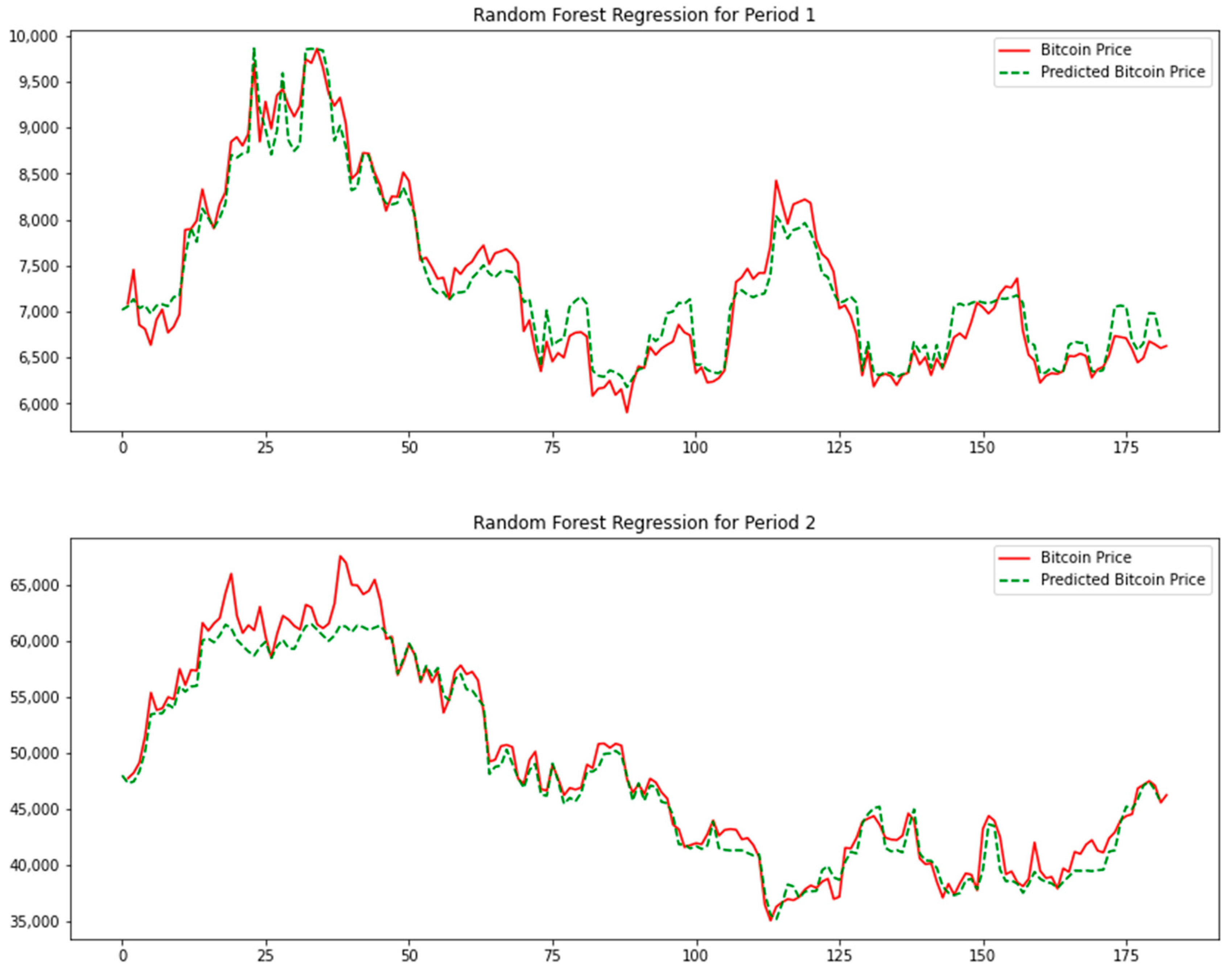
The trained learner is used to predict the test samples of Period 1 and Period 2, and the results shown in

Table 4. Error results for random forest regression.

	Period 1	Period 2
RMSE	321.61	2096.24
MAPE	3.39%	3.29%
DA	51.93%	52.49%

and Figure 8 below are obtained. The red line is the Bitcoin price, and the green dashed line is the price predicted by the random forest regression learner.

Although the RMSE of Period 1 is much smaller than that of Period 2, since the average price of Bitcoin in Period 1 is also much smaller than that of Period 2, it is meaningless to compare the RMSE results of different periods. The MAPE and DA indicators in the two periods are quite close, and the prediction accuracy of Period 2 is slightly better than that of Period 1. It is worth noting that in the early stage of the test interval of Period 2, the random forest regression algorithm has a bad prediction on the Bitcoin price when the price is greater than 60,000 US dollars because there are very few samples with a Bitcoin price greater than USD 60,000 in the training samples of Period 2. This result accurately reflects the disability of the random forest algorithm to predict results outside the training samples. However, whether it is Period 1 or Period 2, the random forest regression algorithm shows excellent performance in predicting prices below USD 60,000, and the trend of the predicted price is consistent with the real price trend.

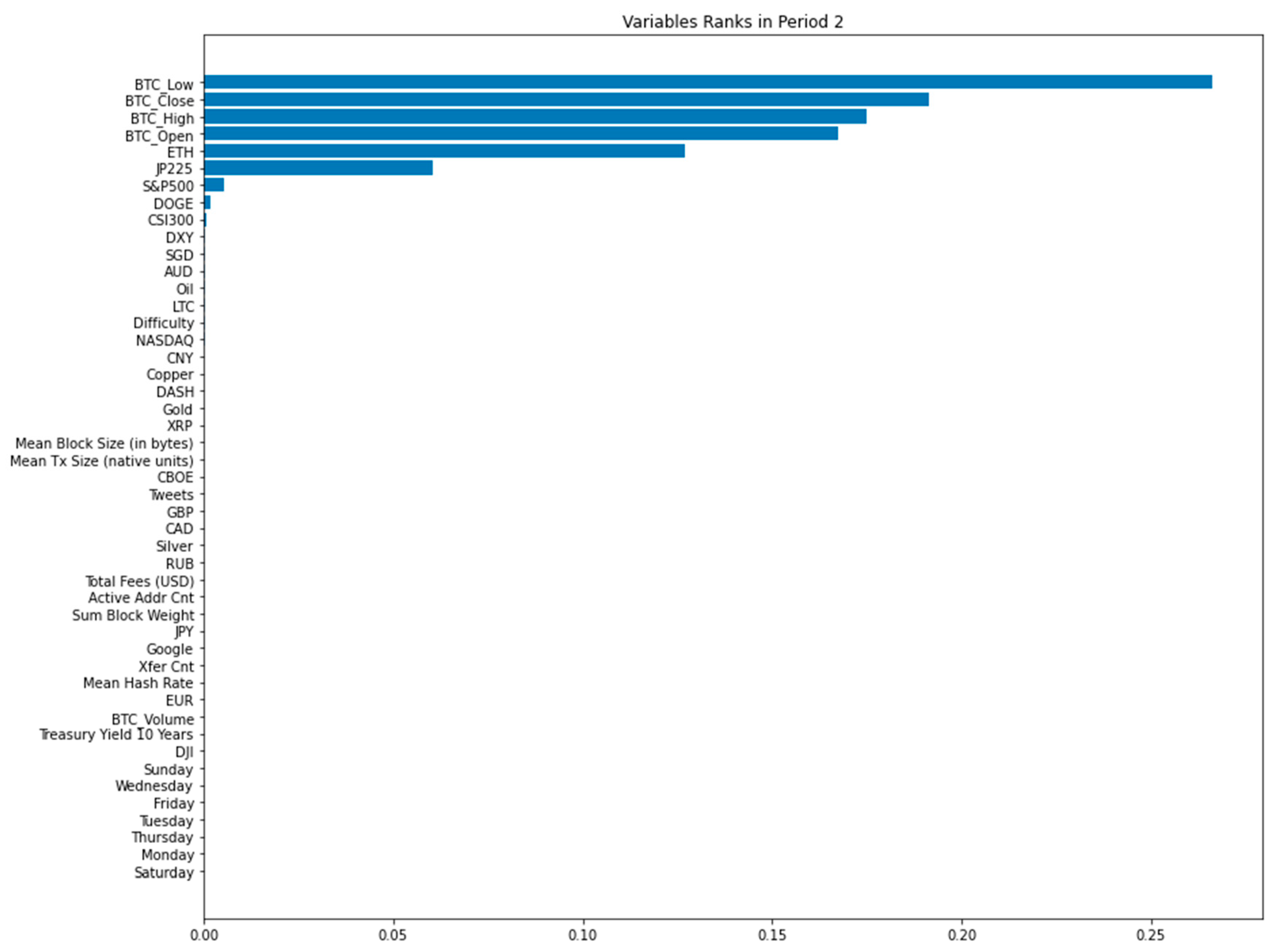
In addition to predictive analysis, the random forest algorithm also provides the importance of each explanatory variable when predicting the price of Bitcoin, through the statistics of the number of occurrences of boundary variables in all 500 sub-regression trees. The result is shown in Figure 9.

Whether it is Period 1 or Period 2, the importance of OHLC price of Bitcoin in the previous period is ranked high. However, what is interesting is that the relative order of open, high, low, and close in the two periods is not the same. According to the random walk theory of sequential prices, the price at each time point reflects the market’s expectation of the future price now, so the closing price closest in time should be the most important item among the four prices. The variable importance results for Period 1 accurately reflect this. However, in the ranking of Period 2, the lowest price of the previous period is considered the most important explanatory variable, and the closing price of the previous period is the last of these four prices. I think the possible reason that the lowest price in the previous period in Period 2 is important is related to the fact that there are more days of Bitcoin price decline in the later period of the Period 2 training sample, and the closing price is not at the highest level also implies that random forest regression delivers different results from random walk theory.

In addition to the variables of Bitcoin’s price, there are several other variables that are evaluated to be important when determining the price of Bitcoin. In Period 1, the NASDAQ index and crude oil prices in the United States are of high importance, even more important than the opening price of Bitcoin. From 7th to 10th places of importance are the American stock market index DJI, S&P500, ETH price, and the difficulty index of mining BTC. Among the top six explanatory variables other than Bitcoin price, the U.S. stock market index accounts for half of the three seats, which reflects the relationship between the U.S. stock market index and Bitcoin price from April 2015 to October 2018.

In Period 2, as shown in the Figure 9, since the importance of GBP in the 7th place is almost negligible, only the first six explanatory variables are considered. Except for the first four Bitcoin price variables, the remaining two are ETH, which is also a cryptocurrency, and Japan’s stock market index JP225.

Regarding the explanatory variables that determine the importance of Bitcoin prices, it can be summarized that the OHLC prices of Bitcoin itself in the previous period are the most important. The importance of the remaining variables changes over time. The stock market index has the highest importance among all major categories. The feature of the high importance of the US stock market index in Period 1 has not been continued in Period 2. The importance of the Japanese stock market increased in Period 2. ETH is the only non-Bitcoin price variable that is considered important for Bitcoin price predictions in both Period 1 and Period 2.

In addition to obtaining the order of importance, to further study the impact of the presence or absence of explanatory variables on the prediction error, two additional tests were performed, which took turns taking out the least important and most important explanatory variable sets, respectively. The results are shown in

Table 5. Summary of explanatory variables importance of Period 1.

Ranking (Period 1)	Normal	Ascending	Descending
1	BTC_Close	BTC_Close	BTC_Close
2	BTC_High	BTC_High	BTC_High
3	NASDAQ	NASDAQ	NASDAQ
4	Oil	BTC_Low	BTC_Low
5	BTC_Low	BTC_Open	BTC_Open
6	S&P500	Oil	DJI
7	BTC_Open	Difficulty	Oil
8	DJI	S&P500	S&P500
9	ETH	DJI	ETH
10	Difficulty	JP225	Difficulty

and

Table 6. Summary of explanatory variables importance of Period 2.

Ranking (Period 2)	Normal	Ascending	Descending
1	BTC_Low	BTC_Low	BTC_Low
2	BTC_High	BTC_High	BTC_High
3	BTC_Close	BTC_Close	BTC_Open
4	BTC_Open	BTC_Open	BTC_Close
5	ETH	ETH	ETH
6	JP225	JP225	JP225
7	S&P500	S&P500	CSI300
8	DOGE	DOGE	AUD
9	CSI300	GBP	NASDAQ
10	DXY	EUR	DXY

below. The normal column is the importance ranking of all explanatory variables in Figure 9. The ascending column is to extract the most important explanatory variables and repeat the experiment. The descending column is to extract the least important explanatory variables and repeat the experiment. The results show that among the top variables in Period 1, except for BTC_Close, BTC_High, NASDAQ, and BTC_Low, all other variables have changed by more than two ranks. In contrast, the ranking of Period 2 is more stable, and the variables from 1 to 6 have not changed except for BTC_Open and BTC_Close.

In addition to the ranking results, I analyzed the change in RMSE after taking out the most important variables in turn. The RMSE corresponding to the variable name on the abscissa refers to the RMSE error after removing it and the upper variables in Figure 10. Therefore, a large range of RMSE changes can show the importance of this variable relative to the remaining variables.

The significant increase in RMSE in Period 1 occurs when BTC_Open is removed. Removing BTC_Open corresponds to removing all OHLC from the previous day data, which shows that when predicting the next Bitcoin price, at least one of the current OHLC Bitcoin price needed. In Period 2, three large changes in RMSE occurred when BTC_Open, ETH, and DOGE were removed separately. Although the result of random forest shows that DOGE appears less often than JP225 and S&P500 in the nodes of all sub- regression trees, the sharp rise in RMSE after removing DOGE shows the effect of DOGE on prediction accuracy. The three large changes in Period 2 are all related to the price variables of cryptocurrency, indicating that the correlation between Bitcoin price and the cryptocurrency market has increased after 2018.

Based on the results about the importance of predicting the price of Bitcoin, I compared the prediction performance between the model with all variables and the model only with important variables (BTC_Close, BTC_High, NASDAQ, and BTC_Low for Period 1; BTC_Close, BTC_High, BTC_Low, BTC_Open, ETH, and JP225 for Period 2). The results show that the prediction accuracy of the model with all explanatory variables is better while the RMSE is 3% smaller than the results using only important variables (Figure 11).

5.2. Results of LSTM

I found that bringing redundant explanatory variables into the model for training leads to a decrease in model accuracy. The accuracy of the model obtained after all 47 explanatory variables are brought in is lower than that of the model using part of the variables, such as the lightweight model using only four Bitcoin price variables. On the contrary, if too few explanatory variables are used, the prediction accuracy of the model also reduces. For example, after adding some other variables to the lightweight model with four Bitcoin price OHLC variables, the prediction accuracy becomes better. Therefore, I have conducted a lot of experiments and attempts on what set of explanatory variables should be substituted in each period. Since there is no such problem in random forest due to it is ensemble algorithm, there is no need to discuss it in random forest regression.

Since the combination of explanatory variables brought in directly affects the prediction accuracy of the model, by referring to the importance rank of the explanatory variables using random forest regression, the respective explanatory variable sets of Period 1 and Period 2 are set in

Table 7. Explanatory variables used in Period 1 and Period 2.

	Period 1	Period 2
Variables	BTC_Open	BTC_Open
	BTC_High	BTC_High
	BTC_Low	BTC_Low
	BTC_Close	BTC_Close
	ETH	ETH
	Oil	JP225
	S&P500
	NASDAQ
	DJI
	Difficulty

.

As the learning results of deep learning are related to the combination of randomly selected learning samples from the sample, randomness was present in the experimental results. Therefore, when comparing the model results, instead of comparing the accuracy of a single model, the average of the results of 30 experiments for various models is compared. The method of comparing the average of multiple experimental results was also applied in the experiments done by Liu et al. (2021).

The one-lagged accuracies of the models for two periods are shown in

Table 8. Errors of the LSTM models.

	Period 1	Period 2
RMSE	330.26	3045.87
MAPE	3.57%	4.68%

Note: the results are the average of 30 runs.

and Figure 12.

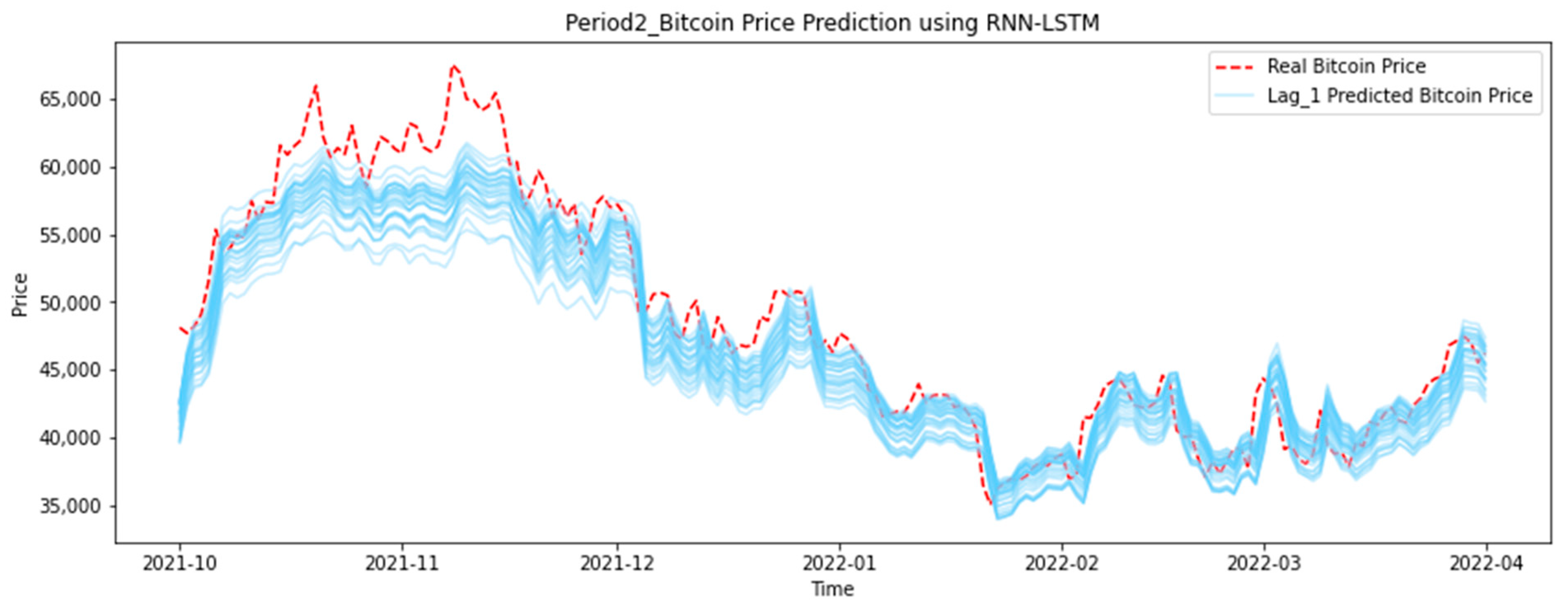
When the Bitcoin price is greater than USD 60,000 in the early period of Period 2, the prediction results of the LSTM algorithm met the same problem of underrating as that in random forest regression. By comparing the MAPE of the two periods, the prediction accuracy of Bitcoin price in Period 1 is better than that in Period 2. This reflects that the correlation between Bitcoin and traditional markets has decreased in recent years, and the randomness of prices has increased. This result also echoes the conclusion that the price correlation is more and more determined by the previous period’s own price, as reflected in the importance ranking of random forest regression in Period 2.

5.3. Relationship between Precision and Number of Variable Periods

Regarding the relationship between model accuracy and the number of lags of explanatory variables, I compared the results of five models with lags from 1 to 5. Whether it is Period 1 or Period 2, the conclusion is that the MAPE of random forest regression increase with the number of periods added as shown in Figure 13. Models trained by only explanatory variable data from the previous period had the best accuracy. This feature of the lagged relationship supports the efficient market hypothesis.

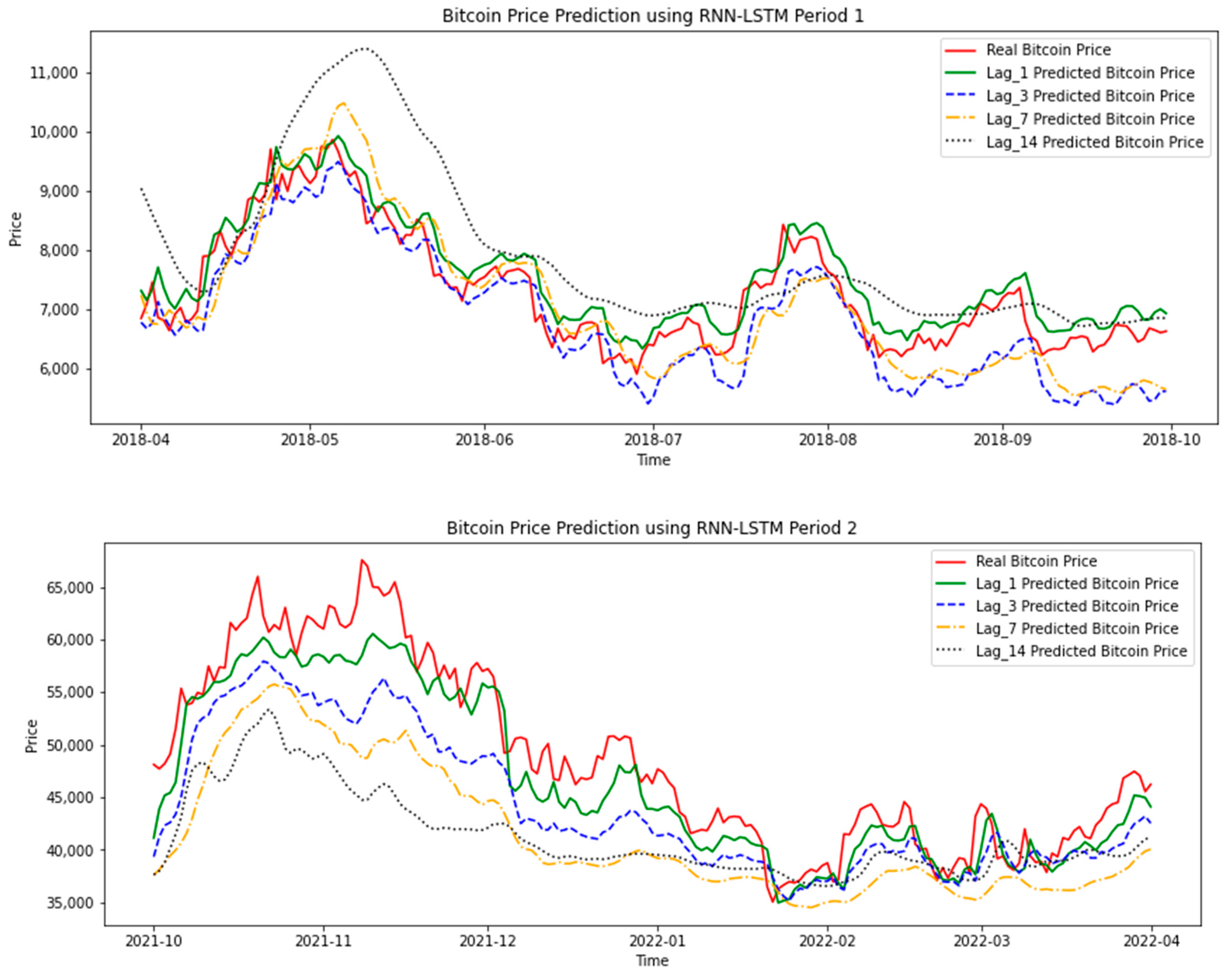
LSTM is a deep learning algorithm with good predictive performance for time series data. The conclusion on whether it is necessary to refer to the data of multiple periods before when predicting the price of Bitcoin is that the prediction accuracy of the model that only needs the previous period is the best. As shown in the results of Period 1 (ten-variable model) and Period 2 (six-variable model) in Figure 14 below, although the price trends of each model are close to real price, the more periods of data substituted into the model, the smoother and smoother the curve of the forecast data becomes, deviating from the real price.

The conclusion on the number of data periods required when training the model is that only using the most recent period of data is sufficient. This conclusion is close to the efficient market hypothesis. The current price reflects the market’s expectation of the future price of the asset, and the price of the previous period has no reference value.

According to summary

Table 9. Model evaluation using the accuracy and error.

		RMSE	MAPE	DA
Period 1	Random forest regression	321.61 (1.67%)	3.39%	51.93%
	LSTM	330.26 (1.71%)	3.57%	49.98%
Period 2	Random forest regression	2096.24 (3.48%)	3.29%	52.49%
	LSTM	3045.87 (5.05%)	4.68%	48.09%

Note: 1. The results are an average of 30 runs. 2. The model of LSTM is the Period 1 ten-variable model and the Period 2 six-variable model. 3. The brackets in the RMSE column are the values that have not been post-processed (min/max).

, it can be found that whether it is Period 1 or Period 2, the price prediction accuracy of the random forest regression model with a lag of 1 is better than that of the LSTM algorithm.

Except for the MAPE index of random forest regression, the other three groups (RMSE of random forest regression, RMSE and MAPE of LSTM) all showed that the prediction error of Period 2 is greater than that of Period 1. This result reflects that the Bitcoin price after October 2018 has become less predictable for the same algorithm. I think this result is related to the fact that the test data of Period 2 is in the bubble period, since machine learning is mainly based on the data of the training model when making predictions. Because the price of the bubble period is too high, the data of historical training are slightly similar, causing the final accuracy declines. This phenomenon is obvious when random forest regression predicts the price of Bitcoin over USD 60,000.

Moreover, the comparison of error values does not reflect the results of hypothesis testing. I used the Diebold–Mariano test and the Clark–West test to further compare the significance of the prediction errors of the random forest regression and LSTM algorithms. The result is that no matter Period 1 or Period 2, the value is not greater than 1.64 required in the case of α = 95%. Thus, it cannot be denied that the prediction accuracy of LSTM is better than that of random forest regression.

Although random forest regression is not significantly better than LSTM, as an algorithm that has not been widely mentioned in the past literature, random forest regression has proven to be equivalent to or even better than LSTM in predicting the price of Bitcoin, as shown in

Table 10. D–M test and C–W test results on the significant difference between random forest regression and LSTM.

	DM Test (MSE)	DM Test (MAE)	Clark and West Test
Period_1	0.36	0.52	0.84
Period_2	0.47	0.47	0.63

Note: when α = 95%, the statistical value of one-tailed test is 1.64.

.

6. Discussion

As a derivative comparison of experimental accuracy,

Table 11. D–M test and C–W test results on the significant difference between random walk and random forest regression or LSTM.

RFR/Random Walk	DM Test (MSE)	DM Test (MAE)	Clark and West Test
Period_1	0.33	0.39	0.58
Period_2	0.55	0.68	0.93
LSTM/random walk	DM test (MSE)	DM test (MAE)	Clark and West test
Period_1	0.34	0.41	0.47
Period_2	0.84	1.15	1.00

Note: when α = 95%, the statistical value of one-tailed test is 1.64.

shows the DM Test and Clark–West test of random forest regression and LSTM relative to the prediction results of random walk. The results of the test show that the prediction accuracy of random walk is worse than that of random forest regression or LSTM and cannot be denied.

There are two directions about future research, shortening the time interval of samples and automation. First, subject to the acquisition of historical data, the unit of the experimental sample this time is daily data, which leads to the prediction of the price has a problem of long interval. Moreover, within 24 h, the possibility of price forecast deviation due to unpredictable problems increases. To avoid the problems caused by the time units discussed above, in the future, I am going to collect the date with intervals of 1 h or 5 min only for the variables with high importance indicators in this experiment. Then, predictive analysis is performed on the new data through random forest regression and LSTM. The second direction of expansion is automation, which can be subdivided into automation of data acquisition and automation of prediction. Regarding the feasibility of Bitcoin predictions, Guarino et al. (2021) have conducted many experiments and believed that the high performance of neural networks in cryptocurrency prediction can be used for transactions. To obtain the predicted price provided by the model at any time, it is necessary to provide the latest data of explanatory variables to the model. A server can be set up on AWS (Amazon Web Services) to collect data prices of various trading websites in real time, and at the same time provide users with the future predicted price of Bitcoin processed by LSTM and random forest regression in the form of an API interface. Moreover, the increase in the number of data collections can also solve the problem of long-time interval.

7. Conclusions

In this paper, to predict the price of Bitcoin on the next day, (a) Bitcoin price variables, (b) the specific technical features of Bitcoin, (c) other cryptocurrencies, (d) commodities, (e) market index, (f) foreign exchange, (g) public attention, and (h) dummy variables of the week, a total of eight categories (47 variables) were used as explanatory variables. Random forest regression has the better price prediction accuracy than LSTM. In previous research, LSTM was widely used and recognized as an algorithm with high accuracy when predicting Bitcoin prices. This paper uses the random forest regression machine learning algorithm, which has not been widely used by other researchers in the previous literature and obtains a result with higher prediction accuracy than LSTM. Although random forest regression has the disadvantage of being unable to predict the results that did not appear in the training samples. For example, when the price of Bitcoin broke the record high, random forest regression could not provide a higher price result than the previous historical high. But with the increase in Bitcoin transaction history, I think random forest regression will perform better when Bitcoin price stabilizes.

As a horizontal comparison with the research that also used daily as the time unit to predict Bitcoin, the RMSE error of random forest regression in this experiment (0.017 in Period 1 and 0.035 in Period 2) is better than is better than 0.045 of LSTM and 0.051 of GRU in Awoke et al.’s (2021) experiment, but worse than 0.009 for SDAE in Liu et al.’s (2021) experiment. I think it is difficult to compare prediction accuracy between different Bitcoin price prediction experiments. First, Bitcoin has many prices bubble periods, and whether the test data is in a bubble period has a great impact. For example, the RMSE error of random forest regression in Period 2 of this study is twice that of Period 1. Secondly, the samples of different unit time cannot be judged by the size of the test error. Interestingly, the models with the best accuracy in Awoke et al.’s (2021) experiments are the models with a lag of seven periods. This result is different from the conclusion in this paper that the optimal model only needs the latest explanatory variables.

The results of random forest regression also show the explanatory variables that determine the price of Bitcoin in various periods. In the first price bubble interval from April 2015 to October 2018, when predicting price on the next day, in addition to the price of the previous period of Bitcoin, the US stock market index (NASDAQ, DJI, and S&P500), the price of oil, ETH price, and the difficulty of finding blocks of Bitcoin, these six variables of mining difficulty also play an important role. During the second price bubble from October 2018 to April 2022, in addition to the OHLC prices of Bitcoin in the previous day, the price of ETH and Japan’s JP225 index act a big role. When predicting the price of Bitcoin greater than USD 60,000 per coin at the end of 2021, random forest regression exposed the problem that it cannot predict values which is not in the training samples. However, the prediction accuracy for the price range below USD 60,000 is good.

In addition to the accuracy conclusion of a single model, the research results also found that whether it is random forest regression or LSTM algorithm, as the number of past periods of the substituted explanatory variables increases, the prediction accuracy of the model decreases. The model with the highest accuracy is the one that only substitutes explanatory variables in the past period. This conclusion is close to the classic efficient market hypothesis.

References

- Aggarwal, Apoorva, Isha Gupta, Novesh Garg, and Anurag Goel. 2019. Deep Learning Approach to Determine the Impact of Socio Economic Factors on Bitcoin Price Prediction. Paper presented at 2019 Twelfth International Conference on Contemporary Computing (IC3), Noida, India, August 8–10. [Google Scholar]
- Akyildirim, Erdinc, Oguzhan Cepni, Shaen Corbet, and Gazi Salah Uddin. 2021. Forecasting mid-price movement of Bitcoin futures using machine learning. Annals of Operations Research, 1–32. [Google Scholar] [CrossRef] [PubMed]
- Awoke, Temesgen, Minakhi Rout, Lipika Mohanty, and Suresh Chandra Satapathy. 2021. Bitcoin Price Prediction and Analysis Using Deep Learning Models. In Communication Software and Networks. Singapore: Springer, pp. 631–40. [Google Scholar]
- Basak, Suryoday, Saibal Kar, Snehanshu Saha, Luckyson Khaidem, and Sudeepa Roy Dey. 2019. Predicting the direction of stock market prices using tree-based classifiers. The North American Journal of Economics and Finance 47: 552–67. [Google Scholar] [CrossRef]
- Baur, Dirk G., and Lai Hoang. 2021. The Bitcoin gold correlation puzzle. Journal of Behavioral and Experimental Finance 32: 100561. [Google Scholar] [CrossRef]
- Baur, Dirk G., and Thomas Dimpfl. 2021. The volatility of Bitcoin and its role as a medium of exchange and a store of value. Empirical Economics 61: 2663–83. [Google Scholar] [CrossRef] [PubMed]
- Blake, R. 2019. An Econometric Analysis of the Relationship between Bitcoin & Gold. Available online: https://medium.com/@blake_richardson/an-econometric-analysis-of-the-relationship-between-bitcoin-gold-2018-584b4c63a17 (accessed on 21 September 2022).
- Carbó, José Manuel, and Sergio Gorjón. 2022. Application of Machine Learning Models and Interpretability Techniques to Identify the Determinants of the Price of Bitcoin. Banco de Espana Working Paper No. 2215. Available online: https://ssrn.com/abstract=4087481 (accessed on 1 October 2022).
- Chen, Wei, Huilin Xu, Lifen Jia, and Ying Gao. 2020a. Machine learning model for Bitcoin exchange rate prediction using economic and technology determinants. International Journal of Forecasting 37: 28–43. [Google Scholar] [CrossRef]
- Chen, Yinghao, Xiaoliang Xie, Tianle Zhang, Jiaxian Bai, and Muzhou Hou. 2020b. A deep residual compensation extreme learning machine and applications. Journal of Forecasting 39: 986–99. [Google Scholar] [CrossRef]
- Derbentsev, Vasily, Natalia Datsenko, Vitalina Babenko, Olha Pushko, and Oleg Pursky. 2020. Forecasting Cryptocurrency Prices Using Ensembles-Based Machine Learning Approach. Paper presented at 2020 IEEE International Conference on Problems of Infocommunications. Science and Technology (PIC S&T), Kharkiv, Ukraine, October 6–9; pp. 707–12. [Google Scholar]
- Erdas, Mehmet Levent, and Abdullah Emre Caglar. 2018. Analysis of the relationships between Bitcoin and exchange rate, commodities and global indexes by asymmetric causality test. Eastern Journal of European Studies 9: 27–45. [Google Scholar]
- Fan, Liwei, Sijia Pan, Zimin Li, and Huiping Li. 2016. An ica-based support vector regression scheme for forecasting crude oil prices. Technological Forecasting and Social Change 112: 245–53. [Google Scholar] [CrossRef]
- García-Medina, Andrés, and Toan Luu Duc Huynh. 2021. What Drives Bitcoin? An Approach from Continuous Local Transfer Entropy and Deep Learning Classification Models. Entropy 23: 1582. [Google Scholar] [CrossRef]
- Guarino, Alfonso, Luca Grilli, Domenico Santoro, Francesco Messina, and Rocco Zaccagnino. 2022. To learn or not to learn? Evaluating autonomous, adaptive, automated traders in cryptocurrencies financial bubbles. Neural Comput & Applic 34: 20715–56. [Google Scholar] [CrossRef]
- Huang, Jia-Yen, and Jin-Hao Liu. 2020. Using social media mining technology to improve stock price forecast accuracy. Journal of Forecasting 39: 104–16. [Google Scholar] [CrossRef]
- Jagannath, Nishant, Tudor Barbulescu, Karam M. Sallam, Ibrahim Elgendi, Asuquo A. Okon, Braden McGrath, Abbas Jamalipour, and Kumudu Munasinghe. 2021. A Self-Adaptive Deep Learning-Based Algorithm for Predictive Analysis of Bitcoin Price. IEEE Access 9: 34054–66. [Google Scholar] [CrossRef]
- Jaquart, Patrick, David Dann, and Christof Weinhardt. 2021. Short-term bitcoin market prediction via machine learning. The Journal of Finance and Data Science 7: 45–66. [Google Scholar] [CrossRef]
- Khan, Wasiat, Mustansar Ali Ghazanfar, Muhammad Awais Azam, Amin Karami, Khaled H. Alyoubi, and Ahmed S. Alfakeeh. 2020. Stock market prediction using machine learning classifiers and social media, news. Journal of Ambient Intelligence and Humanized Computing 13: 3433–56. [Google Scholar] [CrossRef]
- Kim, Alisa, Y. Yang, Stefan Lessmann, Tiejun Ma, M.-C. Sung, and Johnnie E. V. Johnson. 2020a. Can deep learning predict risky retail investors? A case study in financial risk behavior forecasting. European Journal of Operational Research 283: 217–34. [Google Scholar] [CrossRef] [Green Version]
- Kim, Jong-Min, Seong-Tae Kim, and Sangjin Kim. 2020b. On the Relationship of Cryptocurrency Price with US Stock and Gold Price Using Copula Models. Mathematics 8: 1859. [Google Scholar] [CrossRef]
- Lamothe-Fernández, Prosper, David Alaminos, Prosper Lamothe-López, and Manuel A. Fernández-Gámez. 2020. Deep Learning Methods for Modeling Bitcoin Price. Mathematics 8: 1245. [Google Scholar] [CrossRef]
- Liu, Mingxi, Guowen Li, Jianping Li, Xiaoqian Zhu, and Yinhong Yao. 2021. Forecasting the price of Bitcoin using deep learning. Finance Research Letters 40: 101755. [Google Scholar] [CrossRef]
- Livieris, Ioannis E., Niki Kiriakidou, Stavros Stavroyiannis, and Panagiotis Pintelas. 2021. An Advanced CNN-LSTM Model for Cryptocurrency Forecasting. Electronics 10: 287. [Google Scholar] [CrossRef]
- Livieris, Ioannis E., Stavros Stavroyiannis, Emmanuel Pintelas, and Panagiotis Pintelas. 2020. A novel validation framework to enhance deep learning models intime-series forecasting. Neural Computing and Applications 32: 17149–67. [Google Scholar] [CrossRef]
- McNally, Sean, Jason Roche, and Simon Caton. 2018. Predicting the Price of Bitcoin Using Machine Learning. Paper presented at 26th Euromicro International Conference on Parallel, Distributed and Network-Based Processing (PDP), Cambridge, UK, March 21–23; pp. 339–43. [Google Scholar]
- Mudassir, Mohammed, Shada Bennbaia, Devrim Unal, and Mohammad Hammoudeh. 2020. Time-series forecasting of Bitcoin prices using high-dimensional features: A machine learning approach. Neural Computing and Applications, 1–15. [Google Scholar] [CrossRef]
- Nakamoto, Satoshi. 2008. Bitcoin: A Peer-to-Peer Electronic Cash System. Available online: https://bitcoin.org/bitcoin.pdf (accessed on 7 October 2022).
- Parvez, Shaik Javed. 2022. Bitcoin price prediction using Random Forest Regression. Journal of Positive School Psychology 6: 4352–58. [Google Scholar]
- Phaladisailoed, Thearasak, and Thanisa Numnonda. 2018. Machine learning models comparison for bitcoin price prediction. Paper presented at 2018 10th International Conference on Information Technology and Electrical Engineering (ICITEE), Bali, Indonesia, July 24–26; pp. 506–11. [Google Scholar]
- Philip, Richard. 2020. Estimating permanent price impact via machine learning. Journal of Econometrics 215: 414–49. [Google Scholar] [CrossRef]
- Politis, Agis, Katerina Doka, and Nectarios Koziris. 2021. Ether price prediction using advanced deep learning models. Paper presented at 2021 IEEE International Conference on Blockchain and Cryptocurrency (ICBC), Sydney, Australia, May 3–6; pp. 1–3. [Google Scholar]
- Rizwan, Muhammad, Sanam Narejo, and Moazzam Javed. 2019. Bitcoin Price Prediction Using Deep Learning Algorithm. Paper presented at 2019 13th International Conference on Mathematics, Actuarial Science, Computer Science and Statistics (MACS), Karachi, Pakistan, December 14–15; pp. 56–60. [Google Scholar]
- Saadah, Siti, and A. A. Ahmad Whafa. 2020. Monitoring Financial Stability Based on Prediction of Cryptocurrencies Price Using Intelligent Algorithm. Paper presented at 2020 International Conference on Data Science and Its Applications (ICoDSA), Bandung, Indonesia, August 5–6; pp. 1–10. [Google Scholar]
- Sebastião, Helder, and Pedro Godinho. 2021. Forecasting and trading cryptocurrencies with machine learning under changing market conditions. Financial Innovation 7: 1–30. [Google Scholar] [CrossRef] [PubMed]
- Selmi, Refk, Walid Mensi, Shawkat Hammoudeh, and Jamal Bouoiyour. 2018. Is Bitcoin a hedge, a safe haven or a diversifier for oil price movements? A comparison with gold. Energy Economics 74: 787–801. [Google Scholar] [CrossRef]
- Shin, MyungJae, David Mohaisen, and Joongheon Kim. 2021. Bitcoin Price Forecasting via Ensemble-based LSTM Deep Learning Networks. Paper presented at 2021 International Conference on Information Networking (ICOIN), Jeju Island, Republic of Korea, January 13–16; pp. 603–8. [Google Scholar]
- Tandon, Sakshi, Shreya Tripathi, Pragya Saraswat, and Chetna Dabas. 2019. Bitcoin Price Forecasting using LSTM and 10-Fold Cross validation. Paper presented at 2019 International Conference on Signal Processing and Communication (ICSC), Noida, India, March 7–9; pp. 323–28. [Google Scholar] [CrossRef]
Figure 1.
Parameters and framework of random forest regression.
Figure 2.
Parameters and framework of LSTM.
Figure 3.
Training and validation loss of LSTM.
Figure 4.
Correlation heatmap of explanatory variables.
Figure 5.
Google Trend, daily Tweets, and Bitcoin price chart.
Figure 6.
Interval division of training samples and test samples.
Figure 7.
Model employed in this study.
Figure 8.
Predicted price based on random forest regression and actual price comparison.
Figure 9.
Explanatory variable importance ranks using random forest regression.
Figure 10.
RMSE after removing the most important variable.
Figure 11.
RFR results by all variables and only important variables.
Figure 12.
Comparison of the true price of Bitcoin and predicted price based on different models. (LSTM).
Figure 13.
Relationship between MAPE and the number of lags (random forest regression).
Figure 14.
Relationship between accuracy and the number of lags (LSTM).