

An Investigation into the Spatial Distribution of British Housing Market Activity


Department of Accountancy Finance and Economics, University of Lincoln, Lincoln LN6 7TS, UK
J. Risk Financial Manag. 2024, 17(1), 22; https://doi.org/10.3390/jrfm17010022
Submission received: 16 November 2023
/
Revised: 30 December 2023
/
Accepted: 2 January 2024
/
Published: 6 January 2024
(This article belongs to the Special Issue Featured Papers in Mathematics and Finance)
Abstract
:This paper sets out to consider how a simple and easy-to-estimate power-law exponent can be used by policymakers to assess changes in economic inequalities, where the data can have a long tail—common in analyses of economic disparities—yet does not necessarily deviate from log-normality. The paper finds that the time paths of the coefficient of variation and the exponents from Lavalette’s function convey similar inferences about inequalities when analysing the value of house purchases over the period 2001–2022 for England and Wales. The house price distribution ‘steepens’ in the central period, mostly covering the post-financial-crisis era. The distribution of districts’ expenditure on house purchases ‘steepens’ more quickly. This, in part, is related to the loose monetary policy associated with QE driving a wedge between London and the rest of the nation. As prices can rise whilst transactions decline, it may be better for policymakers to focus on the value of house purchases rather than house prices when seeking markers of changes in housing market activity.
1. Introduction
Population nodes are observed to follow a regularity characterised by Zipf’s law, which is a log–log relationship between the rank-size of cities and their corresponding populations. A direct link with central place theory (Hsu 2012) has been made. Cristelli et al. (2012) observe that Zipf’s power law has become a ‘universal’ expression for measuring scale and size in many fields, including economic convergence (Tang et al. 2016), yet the evidence for it is not unequivocal. Perline (2005) is also critical of the widespread use of power laws that may not be the best characterisation of distributions. He argues that some distributions that are believed to follow a power law can be confused with a log-normal distribution if there is substantial truncation.
D’Acci (2023) proposed that the existence of a power law in the distribution of settlement populations should be related to a power law in average house prices, at least in the upper tail. Blackwell (2018) finds limited evidence that house price distributions follow a power law. There is a concession that the tail is fatter than a log-normal one, but not as fat as a ‘true’ power law in data from housing trades in the County of Charleston, South Carolina from 2001 to 2008. It could be that house price data follow a power law in certain price cycle phases. Ohnishi et al. (2020) find the Tokyo house price dispersion is very close to a log-normal distribution in normal times but fits a power function in a boom. They suggest that the shape of the (size-adjusted) price distribution, especially that of the tail, can be investigated for signalling the existence of a bubble.
Fontanelli et al. (2016) note that empirical data often exhibit good power-law distribution within a limited range. Rather than concentrating on where the power law ceases to hold, they modify a power law by changing the functional form. Lavalette’s function is potentially a useful means of describing and quantifying power-law-like behaviours. The Lavalette distribution yields a very good approximation to the log-normal whilst echoing a standard power function, capable of representing long tails. As such, it could address Perline-Blackwell’s critique of applying power functions to log-normal (housing) data.
Van Nieuwerburgh and Weill (2010) find that there is a steeper house price distribution over time. They argue that the driver of spatial house price variations is the city productivity. Behrens et al. (2014) emphasise how productivity affects city size, producing the Zipfian distribution of settlement populations. With productivity also affecting average house prices, a change in the distribution of productivity across space would impact house price inequalities. Van Nieuwerburgh and Weill use a coefficient of variation to assess the steepening spread. The same coefficient is used for sigma-convergence. In the growth literature, this concerns how the distribution (of income) evolves over time (Sala-i-Martin 1996). Gray (2023b) finds that the time profile of the Lavalettean exponents closely tracks that of the coefficient of variation. As both are simple to estimate using, say, Microsoft Excel 2019, the exponent could be quoted alongside the coefficient when presenting cases of growing inequalities to policymakers. This paper considers whether there is ‘a steepening’ or convergence in district house prices and relates this to other measures of housing trades. It compares the results using the coefficient with the exponent.
The paper is structured as follows: First, there is a discussion of central place theory and convergence. Applications of power laws in the fields of price and affordability spreads follow. The significant change in housing transactions following the financial crash is introduced next, plus work that features transactions.
How house prices are expected to vary across space is reviewed with an emphasis on risk. This is followed by drawing a distinction between price changes and expected housing market participation in hot and cold markets. The data analyses are selected for ease of use with widely available software. This includes simple regression. The focus is a Lavalettean expression. Growth is split into the growth of the exponent and the growth of the median. This is adapted to assess the special case of pro-poor growth. The data sources are outlined.
The results show that price and housing market expenditure distributions steepen but these are not linked to a growth period, at odds with Blackwell-Ohnishi et al. A six-year period of relatively rapid price growth before the crash of 2008 is compared with another after the recovery.
2. Literature
The city size regularity characterised by Zipf’s law matches central place theory (Hsu 2012) predictions. Behrens et al. (2014) argue that large cities produce more output per capita than small cities because of a sorting of talented individuals. More talented individuals stand a better chance of becoming highly productive entrepreneurs in larger cities. Correspondingly, there are tougher selection processes in more ‘talented’ cities. Entrepreneurs and firms have better resources to draw from because of the agglomeration economies, boosting productivity, explaining why cities with higher proportions of those with high levels of human capital are larger in equilibrium. Their model generates a Zipfian relationship for city sizes under plausible parameter values.
Cristelli et al. (2012) argue that many real systems do not show true Zipfian behaviour because they are incomplete or inconsistent with the conditions under which one might expect power laws to emerge. A consequence is that, in general, Zipf’s law does not hold for subsets or a union of Zipfian sets. A Zipfian distribution is L-shaped with sizeable outliers at the top end. Perline (2005) points out that it is not uncommon for researchers to truncate the lower tail where the size of the node is small, which could result in some distributions that are believed to follow a power law being confused with log-normal ones.
The notion that a power law in city size has an implication for an associated variable is explored by Rozenfeld et al. (2011), who show that, as well as the population of a node, the footprint of a city also follows a Zipfian distribution. The third leg of the stool, population density, does not. Behrens et al. (2014) predict that, despite urban costs of higher accommodation and commuting time in larger cities, agents do not apportion a greater share of expenditure on housing.
In the field of house prices, D’Acci (2023) finds that Italian regional house prices have a heavy-tailed distribution for which the maximum likelihood estimator suggests a power-law shape is a plausible function for the majority of cases. He suggests that the link is based on per capita income and spatial equilibrium (Roback 1982). This is at odds with the work of Blackwell (2018) who finds limited evidence that house price distributions follow a power law. He concludes that data from housing trades in the County of Charleston, South Carolina from 2001 to 2008 have a fatter tail than log-normal, but not as fat as a ‘true’ power law. This ‘in-between’ possibility is supported when the ‘regular’ power law is compared with the power law with a cut-off. There is some support for a power law with a cut-off. A proposed candidate for exploring this ‘in-between’ zone is a Lavalette function.
Fontanelli et al. (2016) review the properties of the Lavalette function. In their Figure 1 (p. 4) they show how various exponents generate different PDFs. A low value (around −0.1) could generate a bell shape whilst over −0.5, what emerges is something akin to a Zipfian distribution. However, in between, the Lavalette rank function generates a PDF indistinguishable from a log-normal distribution. It is a special case of a discrete generalized beta distribution, which entails estimating two exponents rather than one, which in turn presents estimation complexities, making it less than ideal for simple policy analysis. Lavalette’s special case entails the two exponents being equal. The formula describes a semi-logarithmic S-shape in the cumulative distribution (Chlebus and Divgi 2007). This shape implies that the data should cover the full distribution, not a truncated set. Cerqueti and Ausloos (2015a, 2015b) favour a Lavalettean power law over a Zipfian one for subnational spatial dispersion of Italian tax income. Gray (2022a, 2023b) prefers the Lavalette for subnational inequalities in house prices and affordability ratios over a power law. Using Lavalette’s exponent, he also finds a steepening of spatial house prices and the affordability ratio of England and Wales district distributions. The steepening is between 2006 and 2017. Consistent with the sorting argument seen in Behrens et al. (2014), it is argued that lenders are more willing to advance loans to borrowers in areas attractive to talented individuals, which would strongly favour an extended London area in the UK case. This lending bias could be viewed as reflecting risk-adjusted returns to a dwelling purchase (Gray 2023b; Sinai 2010).
It could be that house price distributions vary with price cycle phases. It is argued that house prices tend to grow faster in larger agglomerations beyond that justified by rents, generating excess returns (Amaral et al. 2021). Mian and Sufi (2018) see the credit-driven household demand channel as distinct from traditional financial accelerator models in explaining house price dynamics, primarily due to the centrality of households in explaining the real effects of credit supply expansions. Lenders inflate the wedge between prices and incomes, which is more likely to leave a permanent effect on high-house-priced areas. Evidence for this can be found in Gray (2022b) who reveals that the time paths of British house price–earnings ratios reflect a spatial divide. The ratios generally rose from a low in 1997 to the bubble period of the 2004–2008 peak. Subsequently, for the South of England, there has been a continuation of this increase, whereas for other areas, the picture is one of relative stability. Rising inequality in England and Wales has two dimensions. Firstly, between the North and South, and secondly among the southern districts.
Bogin et al. (2017) conclude that the price acceleration is a signal of a permanent shift in a location’s economic fundamentals. As the largest nodes at the top end of price hierarchies offering property investment opportunities for a wealthy, international elite (Fernandez et al. 2016), Dublin and London may have decoupled from the rest of the British Isles (Richmond 2007). This suggests a steepening of the price distribution in both countries.
Ohnishi et al. (2020) find the Tokyo house price dispersion is very close to a log-normal distribution in normal times but fits a power function in a boom. They suggest that the shape of the (size-adjusted) price distribution, especially that of the tail, can be investigated for signalling the existence of a bubble. So, one might expect the spatial distribution of house prices to expand in a house price boom.
Hudson and Green (2017) identify that since 2008–2009 there are 400,000 fewer housing transactions taking place each year in the UK compared with the period before the financial crisis, of which 80% could be attributed to a fall in mortgaged home movers. One could argue that this echoes earlier collapses. Andrew and Meen (2003) make a similar point about missing transactions in the 1990s following the 1989 bubble burst. Ortalo-Magné and Rady (2004) suggested that housing market participation in the 1980s among young buyers was unusually high because of credit liberalisation and the rising trend in owner-occupation.
If the housing adjustment following a financial crisis is in transactions, the implications should be of interest to policymakers. Articles featuring house price dispersion and transactions are not common. Tsai (2018) finds the ripple effect in four regional housing markets in the U.S. A ‘ripple’ in transactions was far more evident than that in housing prices. Information is transferred between regional housing markets either through price or volume. The two types of ripple effects are negatively correlated.
Analysing house prices and transactions across European economies, Dröes and Francke (2018) argue that common underlying factors, such as GDP and interest rates, explain part of the price–turnover correlation. The effect of GDP and interest rates mainly operates through turnover. Although a high loan-to-GDP ratio does increase the effect of interest rates and GDP on prices and turnover, it is not considered a key factor in explaining price and turnover dynamics. Similarly, neither population increases, the share of the young population, nor inflation play a central role in this context. They conclude that prices and turnover should be modelled as two interdependent processes. The period 1999–2013 seems unaffected by the drop in participants in 2008, which is not explained.
Clayton et al. (2010) find that price-caused components of prices and volume are negatively correlated. House prices in tight markets are less affected by financial constraints on homebuyers. Dividing the 114 U.S. metropolitan statistical areas into those with high and low supply elasticities, they find that in markets where supply can easily adjust, transaction volume does not seem to affect future prices.
3. Land and Pricing
An asset price model relates the price of a dwelling to the rental stream and the cost of capital, subject to risk adjustments. DiPasquale and Wheaton (1996) analyse factors that affect rent and land prices. The monocentric urban model characterises a collection of dwellings as part of the same housing market area if there is a tendency towards a stable hierarchy of prices. A standard dwelling closer to the central business district will command a higher price ceteris paribus, as owners benefit from the lesser disutility of commuting. The co-movement of prices emerges from ‘arbitrage’; buyers switch search behaviour across the commuting space in the face of mispriced local markets. Relative prices change little as the overall market undergoes either cyclic fluctuations or long-term growth (p. 26). Inter-urban differences in house prices are a function of the relative productivity of areas. Spatial arbitrage operates more generally, as individual agents migrate within and between population nodes to maximise their utility (Roback 1982). This model implies the driver of house price differences is productivity, adjusted for house characteristics and commuting preferences.
The expected future growth in current rent would affect the current local house price (Amaral et al. 2021; DiPasquale and Wheaton 1996; Sinai 2010). This could be due to population growth (DiPasquale and Wheaton 1996; Glaeser and Gyourko 2005), or productivity growth (Coulson et al. 2013; Van Nieuwerburgh and Weill 2010).
Dual regional economy models (Brakman et al. 2020; McCombie 1988) predict slower or constrained growth in the periphery and its elements should have persistently lower productivity. The city’s economic fortunes will be a function of the industries it supports. Martin et al. (2014, 2018) utilise an evolutionary perspective, where agglomeration economies trace out productivity development paths. An ageing economic structure could persistently constrain a city to a poor performance, such as in the northern cities of England that are subject to deindustrialisation (Martin et al. 2018; Pike et al. 2016).
DiPasquale and Wheaton (1996, p. 44) also argue that if the cost of capital falls, this drives up all asset prices. Aimed at mitigating the impact of the financial crisis of 2008, central banks engaged in quantitative easing (QE), which inflated asset prices. The Bank of England’s loose monetary policy, which began with its base rate falling to 0.5% in March 2009, down from 5% in the previous October, was implemented to mitigate the impact of the financial crisis. A longer-run view, due to Miles and Monro (2019), is that there was a sustained decline in real interest rates between 1985 and 2018. Himmelberg et al. (2005) argue that house prices are more sensitive to changes in real interest rates in rapidly growing cities. Amaral et al. (2021) argue that house prices tend to grow faster in major ‘superstar’ cities than what is justified by rents. The excess returns are explained by the lower risk associated with the rents. The distributional impact of QE on measured income and wealth between 2008 and 2014 is assessed as minor in proportional terms. In cash terms, London and the South East gained the most, particularly in housing wealth (Bunn et al. 2018). Indeed, it is averred that London pulls away from the rest of England and Wales (Gray 2018; Montagnoli and Nagayasu 2015; Richmond 2007). This suggests that the price distribution broadened in the aftermath of the crisis due to QE.
A relaxation in credit controls should lead to a surge in demand for dwellings. However, vendors could anticipate this and revise their asking (expected) price upwards before the matching rate increases or the number of transactions surges. Allen and Gale (2000) argue higher price levels are supported by the anticipation of further increases in credit and house prices in general.
4. Transaction–Price–Expenditure Nexus
Ortalo-Magné and Rady (2004) place buyers in a hierarchy, with first-time buyers focussing on more modest dwellings, whereas repeat buyers are looking for larger homes. Smaller dwellings would be traded more frequently than large ones. Smaller dwellings are the first or the only stage in a housing career. Staging could result from a capital constraint or because buyers match their current dwelling with their current space needs. With a variety of divisions of district sizes that are administrative areas rather than markets, the rank order for sales, price levels, and expenditures should not be the same.
Stein’s (1995) model of house prices and transactions focuses on repeat buyers and equity. He analyses the impact of rising prices on three mover groups. The first group relates to those already wishing to buy. A price increase enhances their collateral. Not only does this fortify their purchasing power but, as a lower risk, this would grant them greater access to credit, which leads to further price growth.
The second group, not in the market originally, is induced to sell. As they add liquidity in both buyer and seller markets, they enhance housing market activity (Gray 2023a) and they should speed up the matching process. There are two propositions here. First, as they could now better fund a house purchase, an increase in price, and hence equity, affects the second group much like the first. Novy-Marx (2009) proposes that market participation is related to expected returns and high transaction costs. A more active (hot) market, where buyer–seller matching is quicker, would lower the participation costs for the seller. The bargaining position of either party is dependent on the scarcity of the other. A sudden increase in buyer participation speeds up matching, reducing the pool of sellers that remain, enhancing seller bargaining power, and inflating prices. The buyer ‘shock’ is amplified. Stein asserts that this group does not accelerate prices as they add both demand and supply to the market. In Novy-Marx’s scenario, reduced matching time encourages more vendors to join the market. The greater liquidity lowers the risk to lenders of a fire sale if the marginal buyer gets into difficulties.
The third group needs no credit to buy. Wheaton and Lee (2009) and Ortalo-Magné and Rady (2004) add a buyer with no housing equity to the pool of potential purchasers. This first-time buyer (FTB) is possibly currently renting. This fourth group will behave more like normal consumers, responding to higher prices by withdrawing. The participation of the FTB is necessary for a first-time seller to move on. A fifth group, not featured in Ortalo-Magné and Rady, would include downsizers who look to match space with their reduced family size.
Increased participation is either stimulated by or induces higher prices at lower price levels. However, at some point, the asking prices lead to a diminution of interest from potential buyers, which discourages further sellers from joining the market. Housing expenditure would reflect a combination of market participation and price. In a thick market, an increase in participation is accompanied by price. A thin (cold) market could see prices rising whilst participation declines.
The relaxation of credit should have a greater effect on the highest leveraged markets, most likely with higher market prices. However, permitted leverage will be in the hands of the lender. Where the credit lands during a period of credit loosening is based on risk-adjusted expected returns from a dwelling purchase (Amaral et al. 2021; Sinai 2010). If the current structure of prices has the risk assessment baked in, as reflected in house price–earnings ratios (HPER), the proposition that high-priced districts face a tighter credit constraint could be flawed. It is unclear how a relaxation in credit restrictions could favour a local market. Lenders face agency costs when expanding their loan book. Lenders’ assessment of local risk may be imperfect and backward-looking, which would favour traditionally hotter markets.
Blackwell-Ohnishi et al. suggest that the tail of a house price distribution would contain information about a price bubble. This implies sigma-divergence in the economic growth sense in a boom. It may be better to look to evidence in transactions and sales values when exploring bubbles rather than prices. Loss aversion may obscure dramatic distributional changes in market sentiment. Power-law exponents have been used to characterise convergence (Tang et al. 2016). The Lavalette distribution yields a very good approximation to the log-normal whilst echoing a standard power function, capable of representing long tails (Fontanelli et al. 2016), so it could be used to explore housing distributional changes without making assumptions about power laws that only apply in a boom.
5. Method
A rank-size function can be expressed as where PR is the variable of study (population) and R is the rank score. P1 is that of the largest value, known as the calibrating value, which is that of the largest city and has a rank score of R = 1 with the smallest R = N.
Lavalette’s ranking power law can be expressed as (Gray 2022a). The cross-sectional model is estimated using simple OLS as for R = 1…N for T regressions. The exponentiation of the intercept multiplied by the actual highest value provides the expected CV. The projected median at time t can be calculated from .
Lavalette’s formula allows for the prediction of values other than the median. The projected value at percentile ω, has a power relationship with the median and expected calibrating value E(CV). If q = 0.2 and E(CV) = 100, the median would be 31.6 and the upper quartile value (ω = 75%) would be 41.4. The projected growth rate at the median is defined as . This, at Pω, has two components: the movement of the representative value or median, and the spread. Thus, the growth rate is . The growth rate at certain points in the distribution depends on whether there is convergence or divergence. It is intuitively obvious that steepening occurs when the growth rate at the upper exceeds that at the lower quartile. Indeed, this could predict the acceleration of prices in the tail as implied by Blackwell-Ohnishi et al. The expression , where Y is income, is adapted from Ravallion (2004, p. 6). When poverty reduction is the objective (for which economic growth is one of the instruments) then ‘the rate of pro-poor growth (pp) defined above is the right way to measure growth consistently with that objective’. The distributional correction corresponds with a narrowing of the spread, indicated by the growth at the lower quartile exceeding that of the median and the upper quartile, resulting in convergence.
6. Data
The Local Authority District house prices, incomes, number of transactions, and number of dwellings are supplied by the UK’s Office for National Statistics (ONS) for England and Wales. This covers annual data across 330 districts for the period from 2001 to 2022. The Isles of Scilly are excluded due to intermittent data. All transactions concerning house purchases, whether they entail a loan or not, are captured by these data. The number of transactions reflects the size of the district. To offer some standardisation, this is adjusted by the number of dwellings in the district, generating a sales (or transactions) per dwelling value, which is multiplied by 100,000 (SD). Dröes and Francke (2018) used the same housing stock adjustment to sales. The average house price per district is adjusted by the rate of inflation to provide a real price (RP) based on 2001 levels. The value of sales revenue is the product of the number of transactions and real price. Again, this is weighted by the number of dwellings to provide a measure of housing expenditure (HE).
Figure 1 displays the three variables for four years. The price for 2001 provides the base structure for the displacement of the profile in 2007. The noise in the profile for 2007 relates to the change in order from 2001 to 2007. Generally, low-priced districts in 2001 did not become expensive ones by 2007, yet change is not obviously proportional. Both 2001 and 2007 have the long-tailed S that characterises Lavalette’s law. This is duplicated in 2012/2018 as well as in housing expenditure (HE). Transactions per dwelling also have an S shape, but the long tail is not so pronounced. Also, the number of transactions does not appear to have risen over the first period, and the noise is large relative to the gradient of the profile.
The second period features slower growth. Sales in both 2012 and 2018 appear almost without a gradient, suggesting that if changes in transactions are related to size order this is not much of a claim.
7. Results
There is a concern about misclassifying a distribution when it is quite likely to be log-normal (Perline 2005). The p-values of Kolmogorov–Smirnov goodness of fit test results for selected years are displayed in Table 1. The first consideration is whether the data follow a normal and a log-normal distribution and whether a Lavalette function provides a good fit. Both housing expenditure and price are more likely to follow a log-normal distribution. Sales do not appear log-normal but the case for a normal distribution is not strong. One could infer that there is a good Lavalettean fit for housing expenditure and price. Sales do not consistently follow a distribution considered. In addition, R2 values are reported. A value above 0.98 is linked to a K–S p-value of over 0.05.
The mid-section of Table 1 reports the observed medians for the same selected years. The next three columns report the intercept converted into the estimated median, plus a lower and an upper value based on bootstraps 95% confidence intervals. The observed and estimated values are within 6% of each other, and all the observed values are well within the confidence intervals. Indeed, the estimated median almost duplicates the observed geometric mean (not reported). This relationship is found with log-normal distributions.
7.1. Exponents’ Time Paths
Tsai (2015) finds a segmentation in housing markets between the northern and southern regions. Following this, northern districts/regions, which are defined as the midlands and North of England and Wales, comprise 159 districts. Southern districts or regions comprise London, the East of England, the South West, and the South East. This group contains 171 districts.
The time profiles of coefficients of variation are displayed as a reference in Figure 2 on the left for all districts, North and South. The steepening of prices seen in Gray (2023b) is evident in prices for all districts. This is replicated in housing expenditure, but not in transactions (CoV SD). That said, clearly there are observable narrowing periods. There was another increase in the spread around 2019 to 2021, which pre-dated the lockdown.
Compared with the South, northern districts exhibit a similar range of spread of housing expenditure and transactions, but less variation in price. The profile of all districts’ sales per dwelling is relatively flat until 2007. The subsequent crisis period features a slight broadening of the spread.
On the right-hand side of Figure 2, there are three exponent time paths. Although these are similar to the corresponding CoVs, the patterns are smoother. The price path (q RP) displays the S shape reported by Gray (2023b) but with slightly different dates. The key steepening phase in price runs from 2006 to 2017. There is a period of convergence from 2001 to 2006, and post-2017. The lower section of Table 1 reports the exponents −q for the selected years, plus a lower and an upper value based on bootstraps 95% confidence intervals. The price and housing expenditure coefficients for 2006 are below others, supporting the claims made above concerning convergence and divergence phases.
The S shape is evident in the southern districts’ time profile, but the trough and peak occur earlier. A distinctive feature of the northern districts is the stable distribution after 2010. Here, the S shape is not evident.
The conclusions drawn about steepening depend on the era and the region one selects. Evidence for a steeper distribution is found in the South, not the North of England and Wales post-2008. The rapid steepening from 2008 puts the spread in district expenditure back to a similar position in 2002. The other two spreads return to the 2002 levels around 2009.
The dramatic fall in housing expenditure inequality across all districts covers the initial years to 2005, which is reversed when there is a notable rise in expenditure dispersion from 2008. This again is reversed around 2013, when the RP and HE trajectories lean in opposite directions. Importantly, when clearly rising, HE has steeper trajectories than RP. This is in line with speculative sellers adding liquidity in both buyer and seller markets, enhancing housing market expenditure.
Observed price and quantity values for England and Wales have two distinct patterns at the 2007/2008 juncture. Mean price, adjusted by the rate of inflation, rose to a peak in 2007. It then fell by 5.5% in 2008. The corresponding measure of Hudson and Green’s (2017) missing movers is missing transactions, which entails a propitious drop of 48%. The collapse in expenditure (52%) is greater than sales.
With other consumer durables, one could expect a boost to transactions with a fall in price and lower costs of borrowing. QE’s two elements, increased reserves for banks and lower interest rates, may take some time to penetrate the more risk-averse environment. A downswing in a credit cycle (bust) features a severe restriction of lending, and a rise in collateral requirements (Geanakoplos 2010). Banks withdraw mortgage products and impose larger deposit requirements, which would filter out the higher-risk borrowers, particularly affecting those without property. If loans are not available, offers to buy fall through. If buying one property is contingent on selling the existing one, and that buyer fails to secure funding, both contracts fail to be executed.
Those who bought close to the peak of a price cycle could experience loss aversion (Genesove and Mayer 2001). Unprepared to accept a loss, dwellings could just remain in the estate agent’s window for longer. The speculative participant could withdraw from the market, in part, because the matching rate had dramatically slowed. As such, housing market activity is adversely affected. Hence, the number of house trades and the spatial distribution would be linked to credit and risk appetite.
Transactions per dwelling rate and average district price are lower in the North than in the South. With the exception of the years from 2009 to 2014, there is a negative correlation between district sales/dwelling and price level, in the South. Cheaper districts are associated with more trades. By contrast, the rank order of the district price level is positively associated with that of sales per dwelling in the North for all years apart from 2003 to 2008. Combined, only in 2003 and 2019 are the relationships not positive for the whole of England and Wales, suggesting that more active markets have higher prices.
In general, as measured by the Spearman coefficient, the rank order of district expenditure is strongly linked to price. As shown in Figure 2, the spatial variation in transactions is small compared with that in price. The similarity in the steepening of both the price and expenditure distributions seen in Figure 2 at the national level could reflect this price dominance. Variation at the national level is not reflected in either the South or the North. Moreover, for much of the post-crisis period, price and expenditure distributions of the northern districts are stable, so the ‘steepening’ is more likely to reflect a North–South schism, where the South pulls away from the North, plus greater dispersion in the South.
7.2. Expected Median Time Paths
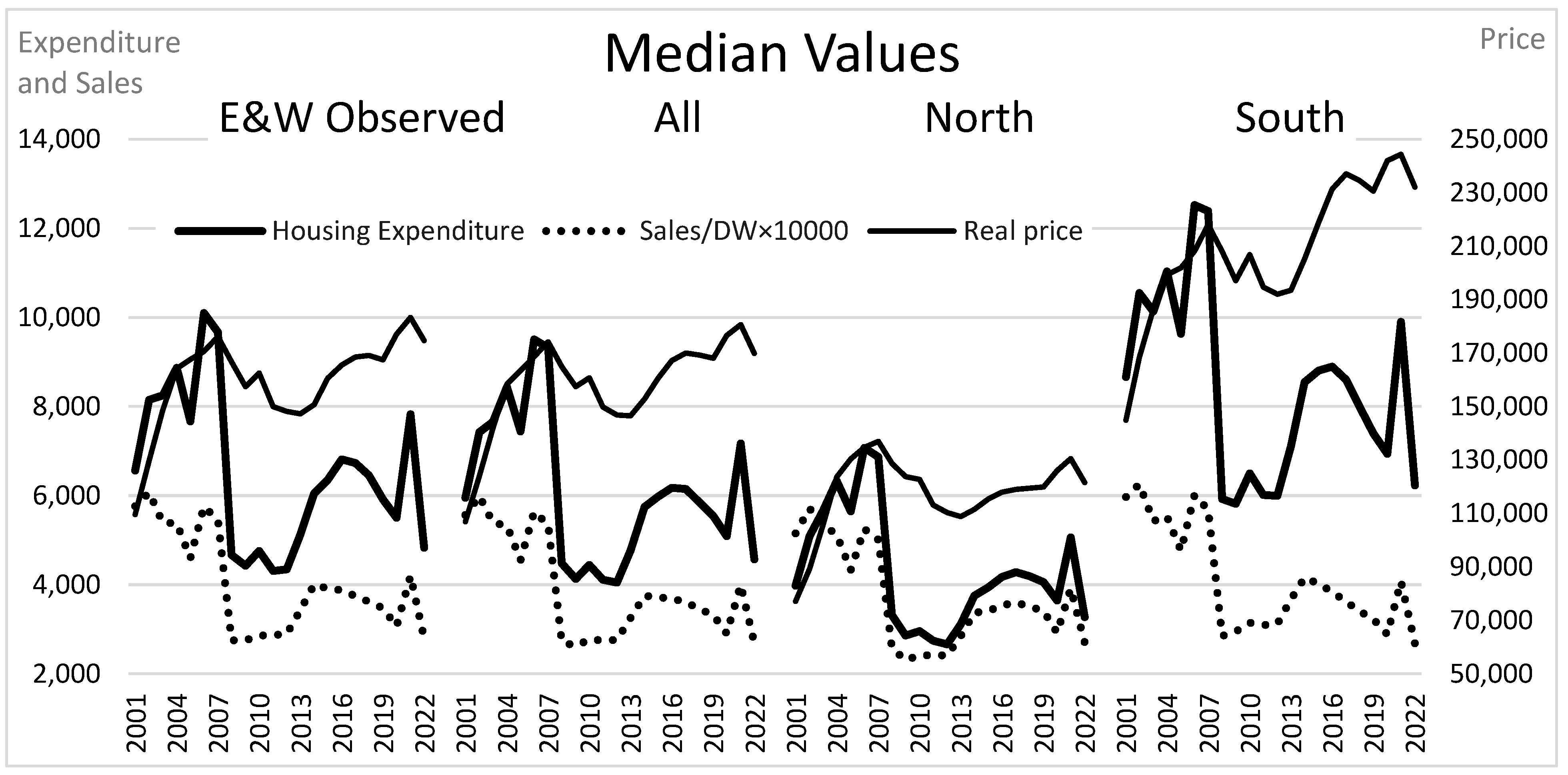
Figure 3 displays the time trajectories of the observed medians of the three measures. There are distinct patterns for price and quantity. The real median price rose to a peak in 2007. It declined by 10% over the period to 2009. This decline continued until 2013. Late in the series, another shock is evident before the COVID-19 lockdown began. It was only then that the price returned to the pre-crisis price level. Up until 2007, there was a general decline in the transactions. The equivalent discussion in the context of Hudson and Green (2017) is that there is no recovery in the number of transactions to the pre-2007 levels. The third line associated with housing expenditure traces the price rising to a peak in 2007. The collapse in expenditure is greater than sales, which it traces from then on. The real pre-COVID-19 price peak occurred in 2018, two years after that found in housing expenditure. Housing expenditure peaked in 2006, a year before price in the pre-financial crisis period. Price peaks occur in cooling markets.
The next three sets of lines are medians as derived from Lavalette’s function for all districts. The patterns of all three sets for each of the three variables concerned are similar to the E&W measures. Both the time profiles of levels (Figure 3) and spreads (Figure 2) correspond well with observations.
7.3. Stein’s Dynamic Framework
For macroprudential purposes, the Bank of England monitors price and affordability (Bank of England 2015). Two six-year periods ending in an inflection point in observed real prices on either side of the financial crisis are analysed. The annualised house price inflation rate at the median from 2012 to 2018 was less than a quarter of the rate from 2001 to 2007 (1.94% < 8.66%). Those districts that had a relatively rapid rise in price in the second period had a slow rate of appreciation in the first (rho = −0.659 [0.000]). By contrast, the growth in expenditure in the first period is positively linked with the second (0.349 [0.000]). This implies that price growth in the second period adversely affected sales growth. Stein’s framework suggests that expenditure and sales should rise over a range of price growth. The rank order of growth rates of expenditure and price are strongly associated in the first period (0.769 [0.000]), but not in the second (−0.065 [0.241]). There is a negative relationship between sales and price (−0.249 [0.000]) in the second period and none in the first. Again, this highlights that activity in the second period is not consistent with the first.
Stein’s framework has been used to explain the divergence in price in the upswing stage of a cycle, with high house prices pulling away from low (Ortalo-Magné and Rady 2004). Spearman’s rho indicates that the growth rates of price over the six years are negatively associated with the price level in the initial year, in the first period (−0.872 [0.000]), but positive in the second (0.502 [0.000]).
Using expenditure data, there is a negative relationship in both the first period (−0.818 [0.000]) and the second (−0.653 [0.000]). This is consistent with the growth literature’s beta-convergence in expenditure (Sala-i-Martin 1996). As the credit cycle enters a looser phase, lenders may cast their eyes around to those areas where less creditworthy debtors might be coaxed onto the market. These areas attract investors’ attention when other opportunities are limited in traditionally lower-risk markets.
The second period, not consistent with Stein’s projection of the co-movement of price and activity could be a result of the distribution of QE funds favouring London (Bunn et al. 2018). Prices in the South reached a point in the post-crisis era where affordability could be beyond what lenders deem as safe, and price is above fundamentals (Duca et al. 2021).
Sigma-convergence entails a narrowing of the distribution over time. Beta-convergence implies that poorer districts grow more quickly than richer ones. Pro-poor growth (Ravallion 2004) implies both. Given a median growth rate, a smaller future Lavalettean exponent implies that the higher housing market values are increasing less quickly than the lower-priced ones, or there is catch-up/pro-poor growth. Table 2 reports observed growth rates at the median and the upper and lower quartiles. These are compared with projected rates based on . In the run-up to 2008, the median price grew by 8.66% annually, which is similar to the Lavalettean projected growth rate (8.47%) within the bootstraps implied confidence interval of 8.34–8.72%. The lower quartile grew faster than the upper (10.45% > 7.08%). The order but not the division is reflected by the expected values (9.54% > 7.41%). All districts and the North and South regions exhibit convergence. This set of results concurs with those using Spearman’s coefficient.
In the second period, again there is a schism between price and expenditure across England and Wales. Convergence is evident when analysing expenditure. House price spreads are consistent with the correlation results and the South pulling away from the North. However, the observed pattern is not consistent when subdivided by North and South, where the North’s distribution narrows whilst the South experiences divergence.
7.4. Stylised Facts
The real price growth rate over the 11 years of the steepening period, 2006–2017, is 0.1% at the median annually and 0.8% at the upper quartile. Expenditure is worse. The annualised contraction rate is 3.2% as opposed to 3.6% at the median. So, the Steinian proposition that higher price growth explains increasing spreads is not supported. It also undermines Blackwell-Ohnishi et al.’s suggestion that the tail of a house price distribution would contain information about a price bubble. Van Nieuwerburgh and Weill (2010) suggest there is a productivity driver of spatial house price variations. Brandily et al. (2022) find that spatial disparities in the UK, although broad, increased slightly up to the financial crisis, but remained generally stable since. Covering 2007–2019, which matches the price steepening period well, Rodrigues and Bridgett (2023) find that London lags behind the rest of the UK in productivity growth, in a low-growth era, implying a narrowing of productivity spreads. London’s productivity grew by 0.2%/ year in real terms, which they suggest is partly a land price problem. They suggest that rising costs for office space deter firms from choosing a location in the City and crowd out investment. High house prices have weakened London’s draw on talented people.
The house price–earnings ratio (HPER) of 4.4 in 2001 rose to 6.96 in 2006. In other words, prices grew by 2.5 annual salaries in a high participation era, or a ‘hot’ market period. Subsequently, the HPER rose nationally to 7.8 in 2017. This is a much smaller increase over a longer period. The continued decline in affordability was accompanied by an extension of the average mortgage repayment period from 25 to 35 years, plus mortgage interest payments were affected by a historically low Bank of England Base rate, leading to the conclusion that monthly mortgage servicing could be steady despite rising house prices. Debt has become dislocated from incomes (Gregoriou et al. 2014). The distribution of QE funds appears to have favoured London (Bunn et al. 2018). Its HPER rose from 7.9 to 12.4 in the period from 2006 to 2017. Affordability metrics in northern regions remain unchanged over that period. Combined, there could be a ‘pulling away of the South’ based on the QE credit dispersion, resulting in the problems highlighted by Gregoriou et al. (2014) and Rodrigues and Bridgett (2023). The QE impact could be spread internationally by a wealthy elite buying up properties in many global centres.
Figure 2 highlights convergence in expenditure across E&W in the post-2013 period whilst prices continued to diverge for the next 4 years. The convergence in expenditure nationally corresponds with markets in the South converging internally plus more rapid growth in (some parts of) the North that catch up. Convergence in the South would not be consistent with a spatial division inflated by a wealthy, international elite, which would focus on London only, reinforcing the QE effect.
7.5. COVID-19
The period from 2019 covering COVID-19 is unusual, as one might expect. The lockdown period began in March 2020 with rapidly declining transactions. Sales in 2020 were at a recent low. Lockdown altered people’s locational preferences. As lockdown restrictions were eased, combined with Stamp Duty holidays, which ended in September 2021, there was a flurry of buyer activity favouring greater space, such as gardens or an extra room for working from home (Hammond 2022; Peachey 2021). The surge in expenditure is evident in Figure 3. With less of an emphasis on commuting, housing market metrics should reflect a dash towards districts with amenities, such as parks and water. Oddly, sales spreads remained stable over this period.
There was a spike in 2021 in both the price and the HPER, yet there is little change in the spread. The impact of the COVID-19 period on house trading activity in the North is almost imperceptible. In 2022, prices and transactions declined as the Bank of England base rate rose from 0.75% to 3.5%. It also announced that it would engage in quantitative tightening, reducing the amount of credit in the system, both of which should reduce market participation. The spread indicators feature a strong narrowing of the distributions.
8. Conclusions
This paper set out to consider the ‘steepness’ of the values of housing transactions as distributed across districts over the period 2001–2022 for England and Wales. The paper finds that the time paths of Lavalette’s (1996) exponents compare well with those of the coefficients of variation. Blackwell (2018) finds that real estate data are ‘in-between’ log-normal and a ‘true’ power law. The distributions of both price and housing expenditure fit that class of data with a long tail, yet often indistinguishable from the log-normal that Lavalette’s law captures. Sales per dwelling do not fit so well. As the exponent is simple to estimate and can provide a meaningful interpretation for data with distributions likely to be found in the worlds of economic inequalities and growth convergence, it has useful properties for the economic policymaker. The exponent produces a time profile akin to the coefficient of variation. This well-used statistic could be inflated as data with a long tail are likely to be skewed and subject to kurtosis, so the exponent could offer a smoother time profile of the dynamics of inequalities.
The paper reveals a Van Nieuwerburgh and Weill ‘steepening’ in the national house price distribution, but this is in the middle of two convergence periods. The first convergence period is associated with the run-up to the financial crisis. Blackwell (2018) and Ohnishi et al. (2020) propose that the upper tail of a house price distribution could contain information about a price bubble. The results here indicate that the distribution is not steepest at the peak price level. Duca et al. (2021) conclude that real-estate-linked financial crises typically begin with over-valued real estate prices. Using risk as an explanation, it is argued that the over-valuation is observed by lenders in southern markets who switch away to less inflated northern ones. The UK’s peak prices nationally occurred as northern price levels ‘caught up’.
Even without a spatial effect, the upper tail may not return to normality quickly due to loss aversion. Prices do adjust downwards but not as dramatically as in activity. Prices can rise in thin markets, ones already experiencing a significant drop in financial transactions. As such, it is argued that evidence of volatile housing market activity is better found in housing transaction expenditure, which peaked earlier than prices in both pre- and post-crisis periods. Housing expenditure is found to steepen more rapidly than prices, in a period of low market participation and lower real activity. Again, the upper tail in price would not offer an insight into an over-heated housing market. There is a period when there is convergence in expenditure and divergence in price. The schism between housing expenditure and price, particularly post-2013, would be consistent with a peak price occurring in a cooling market nationally. A thick market in the North could coexist with a thin market but with rising prices in the South.
Macroprudential regulation seeks to limit reckless lending with national metric lending rules (Bank of England 2015) based on price growth and affordability. Rather than productivity, it is averred that lending and QE funds favouring London (Bunn et al. 2018) underpinned the steepening across the UK. The post-financial-crisis price patterns understate the extent of depressed market activity compared with before. QE may have ossified prices at damaging levels in the South, affecting productivity growth itself, the driver of spreads (Van Nieuwerburgh and Weill 2010) elsewhere. Monitoring of housing activity could be improved by analysing housing expenditure, which should be a lead indicator and more in line with lending activity.
Funding
This research received no external funding.
Data Availability Statement
Data is freely available from government agency websites.
Conflicts of Interest
The author declares no conflict of interest.
References
- Allen, Franklin, and Douglas Gale. 2000. Bubbles and crises. The Economic Journal 110: 236–55. [Google Scholar] [CrossRef]
- Amaral, Francisco, Martin Dohmen, Sebastian Kohl, and Moritz Schularick. 2021. Superstar Returns. The New York Federal Staff Reports 999. New York: Federal Reserve Bank of New York. [Google Scholar] [CrossRef]
- Andrew, Mark, and Geoffrey Meen. 2003. House Price Appreciation, Transactions and Structural Change in the British Housing Market: A Macroeconomic Perspective. Real Estate Economics 31: 99–116. [Google Scholar] [CrossRef]
- Bank of England. 2015. The Financial Policy Committee’s Powers over Housing Tools. Available online: https://www.bankofengland.co.uk/-/media/boe/files/statement/2015/the-financial-policy-committees-powers-over-housing-tools.pdf?la=en&hash=824555A3E0E43904679511189F70706FC5EE5EA2 (accessed on 1 February 2018).
- Behrens, Kristian, Gilles Duranton, and Frédéric Robert-Nicoud. 2014. Productive Cities: Sorting, Selection, and Agglomeration. Journal of Political Economy 122: 507–53. [Google Scholar]
- Blackwell, Calvin. 2018. Power Laws in Real Estate Prices? Some Evidence. The Quarterly Review of Economics and Finance 69: 90–98. [Google Scholar] [CrossRef]
- Bogin, Alexander, William Doerner, and William Larson. 2017. Local House Price Paths: Accelerations, Declines, and Recoveries. The Journal of Real Estate Finance and Economics 58: 201–22. [Google Scholar] [CrossRef]
- Brakman, Steven, Harry Garretsen, and Charles van Marrewijk. 2020. An Introduction to Geographical and Urban Economics: A Spiky World. Cambridge: Cambridge University Press. [Google Scholar]
- Brandily, Paul, Mimosa Distefano, Hélène Donnat, Immanuel Feld, Henry G. Overman, and Krishan Shah. 2022. Bridging the Gap: What Would It Take to Narrow the UK’s Productivity Disparities? Resolution Foundation. Available online: https://economy2030.resolutionfoundation.org/wp-content/uploads/2022/06/Bridging-the-gap.pdf (accessed on 1 November 2022).
- Bunn, Philip, Alice Pugh, and Chris Yeates. 2018. The Distributional Impact of Monetary Policy Easing in the UK between 2008 and 2014. March Staff Working Paper No. 720. Available online: https://www.bankofengland.co.uk/news/publications (accessed on 1 September 2022).
- Cerqueti, Roy, and Marcel Ausloos. 2015a. Cross ranking of cities and regions: Population versus income. Journal of Statistical Mechanics: Theory and Experiment 2015: P07002. [Google Scholar] [CrossRef]
- Cerqueti, Roy, and Marcel Ausloos. 2015b. Evidence of economic regularities and disparities of Italian regions from aggregated tax income size data. Physica A: Statistical Mechanics and Its Applications 421: 187–207. [Google Scholar] [CrossRef]
- Chlebus, Edward, and Gautam Divgi. 2007. A Novel Probability Distribution for Modeling Internet Traffic and its Parameter Estimation. Paper presented at IEEE Global Telecommunications Conference Global Telecommunications Conference, IEEE GLOBECOM Proceedings: 4670–4075, Washington, DC, USA, 26–30 November; Available online: https://ieeexplore.ieee.org/document/4411796 (accessed on 1 September 2022).
- Clayton, Jim, Norman Miller, and Liang Peng. 2010. Price-volume Correlation in the Housing Market: Causality and Co-movements. The Journal of Real Estate Finance and Economics 40: 14–40. [Google Scholar] [CrossRef]
- Coulson, N. Edward, Crocker H. Liu, and Sriram V. Villupuram. 2013. Urban economic base as a catalyst for movements in real estate prices. Regional Science and Urban Economics 43: 1023–40. [Google Scholar] [CrossRef]
- Cristelli, Matthieu, Michael Batty, and Luciano Pietronero. 2012. There is more than a power law in Zipf. Scientific Reports 2: 812. [Google Scholar] [CrossRef] [PubMed]
- D’Acci, Luca S. 2023. Is housing price distribution across cities, scale invariant? Fractal distribution of settlements’ house prices as signature of self-organized complexity. Choas Solitons and Fractals 174: 113766. [Google Scholar] [CrossRef]
- DiPasquale, Denise, and William Wheaton. 1996. Urban Economics and Real Estate Markets. Englewood Cliffs: Prentice Hall. [Google Scholar]
- Dröes, Martijn, and Marc Francke. 2018. What Causes the Positive Price-Turnover Correlation in European Housing Markets? The Journal of Real Estate Finance and Economics 57: 618–46. [Google Scholar] [CrossRef]
- Duca, John, John Muellbauer, and Anthony Murphy. 2021. What Drives House Price Cycles? International Experience and Policy Issues. Journal of Economic Literature 59: 773–864. [Google Scholar] [CrossRef]
- Fernandez, Rodrigo, Annelore Hofman, and Manuel B. Aalbers. 2016. London and New York as a Safe Deposit Box for the Transnational Wealth Elite. Environment and Planning A 48: 2443–61. [Google Scholar]
- Fontanelli, Oscar, Pedro Miramontes, Yaning Yang, Germinal Cocho, and Wentian Li. 2016. Beyond Zipf’s Law: The Lavalette Rank Function and Its Properties. PLoS ONE 11: e0163241. [Google Scholar] [CrossRef]
- Geanakoplos, John. 2010. Solving the Present Crisis and Managing the Leverage Cycle. New York Federal Reserve Economic Policy Review 16: 101–31. [Google Scholar] [CrossRef]
- Genesove, David, and Christopher Mayer. 2001. Loss aversion and seller behavior: Evidence from the housing market. Quarterly Journal of Economics 87: 1233–60. [Google Scholar] [CrossRef]
- Glaeser, Edward L., and Joseph Gyourko. 2005. Urban Decline and Durable Housing. Journal of Political Economy 113: 345–75. [Google Scholar] [CrossRef]
- Gray, David. 2018. Convergence and divergence in British housing space. Regional Studies 52: 901–10. [Google Scholar] [CrossRef]
- Gray, David. 2022a. Do House Price-Earnings Ratios in England and Wales follow a Power Law? An Application of Lavalette’s Law to District Data. Environment and Planning B: Urban Analytics and City Science 49: 1184–96. [Google Scholar] [CrossRef]
- Gray, David. 2022b. How Have District-Based House Price-Earnings Ratios Evolved in England and Wales? Journal of Risk and Financial Management 15: 351. [Google Scholar] [CrossRef]
- Gray, David. 2023a. Housing market activity diffusion in England and Wales. National Accounting Review 5: 125–44. [Google Scholar] [CrossRef]
- Gray, David. 2023b. Power Laws and Inequalities: The Case of British District House Price Dispersion. Risks 11: 136. [Google Scholar] [CrossRef]
- Gregoriou, Andros, Alexandros Kontonikas, and Alberto Montagnoli. 2014. Aggregate and regional house price to earnings ratio dynamics in the UK. Urban Studies 51: 2916–27. [Google Scholar] [CrossRef]
- Hammond, George. 2022. Is the UK Housing Market at a Turning Point? Financial Times, August 12. [Google Scholar]
- Himmelberg, Charles, Christopher Mayer, and Todd Sinai. 2005. Assessing High House Prices: Bubbles, Fundamentals and Misperceptions. Journal of Economic Perspectives 19: 67–92. [Google Scholar] [CrossRef]
- Hsu, Wen-Tai. 2012. Central Place Theory and City Size Distribution. The Economic Journal 122: 903–32. [Google Scholar] [CrossRef]
- Hudson, Neal, and Brian Green. 2017. Missing Movers: A Long-Term Decline in Housing Transactions? Council of Mortgage Lenders. Available online: https://thinkhouse.org.uk/site/assets/files/1756/cmlmissing.pdf (accessed on 1 September 2022).
- Lavalette, Daniel. 1996. Facteur D’impact: Impartialité ou Impuissance? Orsay: Internal Report INSERM U350 Institut Curie—Recherche, Bât. 112, Centre Universitaire. Available online: http://www.curie.u-psud.fr/U350/ (accessed on 1 September 2022).
- Martin, Ron, Ben Gardiner, and Peter Tyler. 2014. The Evolving Economic Performance of UK Cities: City Growth Patterns, 1981–2011; Working Paper, Foresight Programme on The Future of Cities. London: UK Government Office for Science, Department of Business, Innovation and Skills.
- Martin, Ron, Peter Sunley, Ben Gardiner, Emil Evenhuis, and Peter Tyler. 2018. The city dimension of the productivity growth puzzle: The relative role of structural change and within-sector slowdown. Journal of Economic Geography 18: 539–70. [Google Scholar] [CrossRef]
- McCombie, John. 1988. A synoptic view of regional growth and unemployment: II The post-Keynesian theory. Urban Studies 25: 399–417. [Google Scholar] [CrossRef]
- Mian, Atif, and Amir Sufi. 2018. Finance and Business Cycles: The Credit-Driven Household Demand Channel. Journal of Economic Perspectives 32: 31–58. [Google Scholar] [CrossRef]
- Miles, David, and Victoria Monro. 2019. UK House Prices and Three Decades of Decline in the Risk Free Real Interest Rate, Staff Working Paper No. 837. London: Bank of England. [Google Scholar]
- Montagnoli, Alberto, and Jun Nagayasu. 2015. UK house price convergence clubs and spillovers. Journal of Housing Economics 30: 50–58. [Google Scholar] [CrossRef]
- Novy-Marx, Robert. 2009. Hot and Cold Markets. Real Estate Economics 37: 1–22. [Google Scholar] [CrossRef]
- Ohnishi, Takaaki, Takayuki Mizuno, and Tsutomu Watanabe. 2020. House price dispersion in boom–bust cycles: Evidence from Tokyo. The Japanese Economic Review 71: 511–39. [Google Scholar] [CrossRef]
- Ortalo-Magné, François, and Sven Rady. 2004. Housing transactions and macroeconomic fluctuations: A case study of England and Wales. Journal of Housing Economics 13: 287–303. [Google Scholar] [CrossRef]
- Peachey, Kevin. 2021. How COVID Has Changed Where We Want to Live. BBC News, March 19. [Google Scholar]
- Perline, Richard. 2005. Strong, Weak and False Inverse Power Laws. Statistical Science 20: 68–88. Available online: http://www.jstor.org/stable/20061161 (accessed on 1 September 2022). [CrossRef]
- Pike, Andy, Danny MacKinnon, Mike Coombes, Tony Champion, David Bradley, Andrew Cumbers, Liz Robson, and Colin Wymer. 2016. Uneven Growth: Tackling City Decline. New York: Joseph Rowntree Foundation. Available online: https://www.jrf.org.uk/report/uneven-growth-tackling-city-decline (accessed on 8 August 2023).
- Ravallion, Martin. 2004. Pro-Poor Growth: A Primer. Policy Research Working Paper; No. 3242. Washington, DC: World Bank. Available online: http://hdl.handle.net/10986/14116 (accessed on 8 August 2023).
- Richmond, Peter. 2007. A roof over your head; house price peaks in the UK and Ireland. Physica A: Statistical Mechanics and its Applications 375: 281–87. [Google Scholar] [CrossRef]
- Roback, Jennifer. 1982. Wages, Rents, and the Quality of Life. Journal of Political Economy 90: 1257–78. Available online: https://www.jstor.org/stable/1830947 (accessed on 1 September 2022). [CrossRef]
- Rodrigues, Guilherme, and Stuart Bridgett. 2023. Capital Losses: The Role of London in the UK’s Productivity Puzzle. Centre for Cities’ Report. March 2. Available online: https://www.centreforcities.org/press/londons-productivity-lags-well-behind-global-competitors/ (accessed on 1 September 2022).
- Rozenfeld, Hernan, Diego Rybski, Xavier Gabaix, and Hernan Makse. 2011. The Area and Population of Cities: New Insights from a Different Perspective on Cities. The American Economic Review 101: 2205–25. [Google Scholar] [CrossRef]
- Sala-i-Martin, Xavier. 1996. Regional cohesion: Evidence and theories of regional growth and convergence. European Economic Review 40: 1325–52. [Google Scholar] [CrossRef]
- Sinai, Todd. 2010. Feedback Between Real Estate and Urban Economics. Journal of Regional Science 50: 423–48. [Google Scholar] [CrossRef]
- Stein, Jeremy. 1995. Prices and trading volume in the housing market: A model with downpayment effects. The Quarterly Journal of Economics 110: 379–405. [Google Scholar] [CrossRef]
- Tang, Pan, Ying Zhang, Belal E. Baaquie, and Boris Podobnik. 2016. Classical convergence versus Zipf rank approach: Evidence from China’s local-level data. Physica A: Statistical Mechanics and its Applications 443: 246–53. [Google Scholar] [CrossRef]
- Tsai, I-Chun. 2015. Spillover Effect between the Regional and the National Housing Markets in the UK. Regional Studies 49: 1957–76. [Google Scholar] [CrossRef]
- Tsai, I-Chun. 2018. The cause and outcomes of the ripple effect: Housing prices and transaction volume. The Annals of Regional Science 61: 351–73. [Google Scholar] [CrossRef]
- Van Nieuwerburgh, Stijn, and Pierre-Olivier Weill. 2010. Why Has House Price Dispersion Gone Up? The Review of Economic Studies 77: 1567–606. [Google Scholar] [CrossRef]
- Wheaton, William, and Nai Lee. 2009. The Co-Movement of Housing Sales and Housing Prices: Empirics and Theory. SSRN Electronic Journal. [Google Scholar] [CrossRef]
Figure 1.
The distribution of housing expenditure, sales and real price.
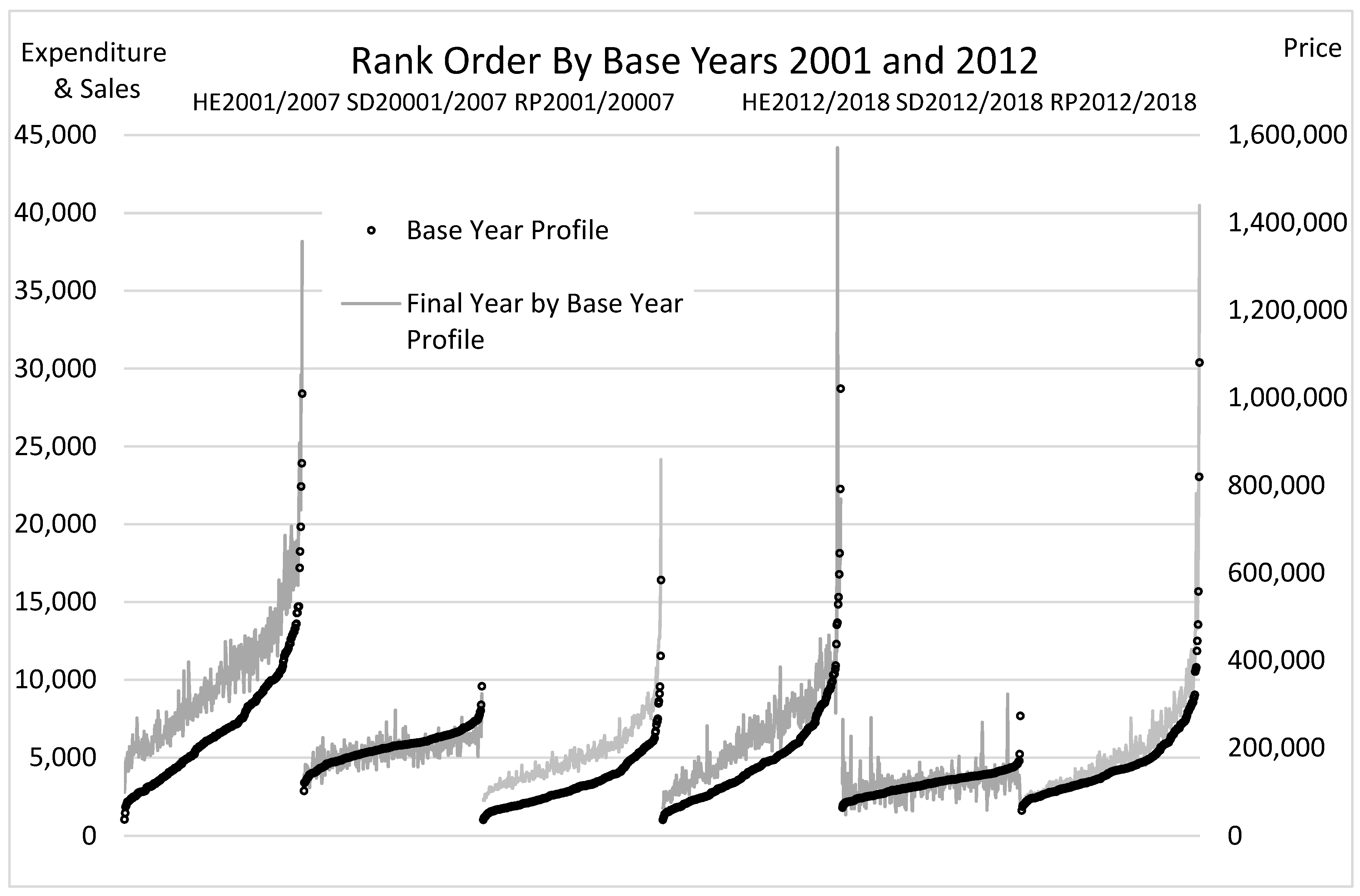
Figure 2.
Time paths of spread measures.
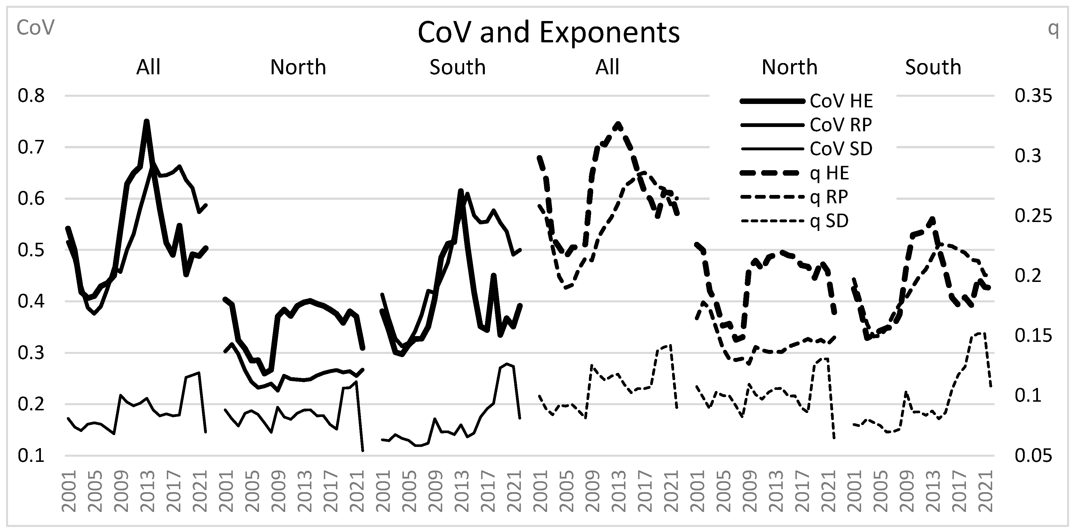
Figure 3.
Median values: price transactions and expenditure.

Table 1.
Goodness of fit, medians, and exponents. Obs = observed; Est = estimated; BS L = bootstraps lower band; BS U = bootstraps upper band; p-values * sig. at the 5% level ** sig. at the 1% level.
Table 1.
Goodness of fit, medians, and exponents. Obs = observed; Est = estimated; BS L = bootstraps lower band; BS U = bootstraps upper band; p-values * sig. at the 5% level ** sig. at the 1% level.
| Housing Expenditure (Price × Sales/D) | Real Price | Sales/Dwelling × 10,000 | ||||||||||
|---|---|---|---|---|---|---|---|---|---|---|---|---|
| K–S | Laval Ette | R2 | Normal | Log-Normal | Laval Ette | R2 | Normal | Log-Normal | Laval Ette | R2 | Normal | Log-Normal |
| Kolmogorov–Smirnov | ||||||||||||
| 2001 | 0.579 | 0.982 | 0.00 ** | 0.014 * | 0.645 | 0.979 | 0.00 ** | 0.20 | 0.26 | 0.982 | 0.20 | 0.00 ** |
| 2006 | 0.774 | 0.986 | 0.00 ** | 0.20 | 0.645 | 0.982 | 0.00 ** | 0.20 | 0.46 | 0.984 | 0.20 | 0.00 ** |
| 2007 | 0.579 | 0.986 | 0.00 ** | 0.20 | 0.774 | 0.975 | 0.00 ** | 0.20 | 0.30 | 0.986 | 0.20 | 0.007 ** |
| 2009 | 0.710 | 0.984 | 0.00 ** | 0.20 | 0.049 * | 0.967 | 0.00 ** | 0.004 ** | 0.032 * | 0.949 | 0.00 ** | 0.00 ** |
| 2012 | 0.516 | 0.983 | 0.00 ** | 0.20 | 0.06 | 0.959 | 0.00 ** | 0.003 ** | 0.09 | 0.962 | 0.036 * | 0.00 ** |
| 2014 | 0.456 | 0.982 | 0.00 ** | 0.06 | 0.109 | 0.949 | 0.00 ** | 0.00 ** | 0.004 ** | 0.942 | 0.00 ** | 0.00 ** |
| 2018 | 0.516 | 0.979 | 0.00 ** | 0.022 * | 0.456 | 0.964 | 0.00 ** | 0.015 * | 0.13 | 0.932 | 0.034 * | 0.00 ** |
| 2022 | 0.456 | 0.980 | 0.00 ** | 0.07 | 0.516 | 0.972 | 0.00 ** | 0.07 | 0.002 ** | 0.879 | 0.00 ** | 0.00 ** |
| Median Values | ||||||||||||
| Obs | Est | BS L | BS U | Obs | Est | BS L | BS U | Obs | Est | BS L | BS U | |
| 2001 | 6294 | 5951 | 5758 | 6207 | 104,810 | 106,933 | 102,535 | 111,409 | 5730 | 5566 | 5466 | 5667 |
| 2006 | 9755 | 9509 | 9275 | 9770 | 167,172 | 168,706 | 162,741 | 176,119 | 5738 | 5636 | 5564 | 5710 |
| 2007 | 9222 | 9318 | 9070 | 9592 | 172,507 | 174,176 | 165,847 | 184,024 | 5453 | 5350 | 5291 | 5409 |
| 2009 | 4198 | 4133 | 3995 | 4293 | 154,134 | 157,485 | 148,909 | 167,391 | 2692 | 2624 | 2534 | 2729 |
| 2012 | 4185 | 4052 | 3874 | 4255 | 144,349 | 146,928 | 136,039 | 159,803 | 2828 | 2758 | 2674 | 2842 |
| 2014 | 5935 | 5747 | 5483 | 6048 | 146,518 | 152,864 | 140,548 | 166,925 | 3922 | 3760 | 3656 | 3878 |
| 2018 | 6188 | 5858 | 5606 | 6214 | 161,986 | 169,294 | 156,905 | 182,115 | 3596 | 3460 | 3341 | 3602 |
| 2022 | 4688 | 4569 | 4372 | 4784 | 168,992 | 169,914 | 160,339 | 180,060 | 2781 | 2689 | 2586 | 2810 |
| Exponents (-q) | ||||||||||||
| Est | BS L | BS U | Est | BS L | BS U | Est | BS L | BS U | ||||
| 2001 | 0.298 | 0.292 | 0.305 | 0.251 | 0.243 | 0.259 | 0.100 | 0.097 | 0.103 | |||
| 2006 | 0.224 | 0.219 | 0.228 | 0.188 | 0.181 | 0.195 | 0.092 | 0.090 | 0.094 | |||
| 2007 | 0.224 | 0.219 | 0.229 | 0.197 | 0.189 | 0.207 | 0.087 | 0.085 | 0.089 | |||
| 2009 | 0.284 | 0.277 | 0.291 | 0.202 | 0.192 | 0.212 | 0.125 | 0.120 | 0.131 | |||
| 2012 | 0.319 | 0.31 | 0.328 | 0.231 | 0.218 | 0.245 | 0.116 | 0.112 | 0.121 | |||
| 2014 | 0.317 | 0.308 | 0.326 | 0.250 | 0.236 | 0.266 | 0.109 | 0.104 | 0.114 | |||
| 2018 | 0.263 | 0.255 | 0.273 | 0.263 | 0.250 | 0.276 | 0.107 | 0.101 | 0.114 | |||
| 2022 | 0.251 | 0.243 | 0.260 | 0.248 | 0.238 | 0.259 | 0.088 | 0.081 | 0.096 | |||
Table 2.
Annualised growth rates over two growth periods: price, transactions, and expenditure.
| 2001–2007 (1) 2012–2018 (2) | All Districts | North | South | ||||||
|---|---|---|---|---|---|---|---|---|---|
| Real Exp/Dw | Sale/Dw | Real Price | Real Exp/Dw | Sale/Dw | Real Price | Real Exp/Dw | Sale/Dw | Real Price | |
| Observed (1) | |||||||||
| Lower Q | 9.27 | −0.34 | 10.45 | 11.72 | −0.33 | 10.56 | 6.75 | −0.97 | 7.63 |
| Median | 6.57 | −0.82 | 8.66 | 9.54 | −0.55 | 10.46 | 5.91 | −0.50 | 6.96 |
| Upper Q | 5.27 | −1.02 | 7.08 | 7.80 | −0.84 | 8.91 | 5.57 | −1.14 | 5.91 |
| Estimated (1) | |||||||||
| Lower Q | 9.24 | −0.43 | 9.54 | 11.12 | −0.17 | 10.72 | 6.77 | −0.73 | 7.64 |
| Median | 7.76 | −0.66 | 8.47 | 9.51 | −0.46 | 10.02 | 6.15 | −0.84 | 7.05 |
| Upper Q | 6.3 | −0.89 | 7.41 | 7.93 | −0.75 | 9.32 | 5.53 | −0.95 | 6.47 |
| Observed (2) | |||||||||
| Lower Q | 8.26 | 4.82 | 1.50 | 7.89 | 6.92 | 1.01 | 5.73 | 1.66 | 3.29 |
| Median | 6.74 | 4.09 | 1.94 | 8.28 | 6.40 | 1.32 | 5.24 | 2.17 | 3.38 |
| Upper Q | 5.31 | 3.30 | 3.52 | 8.44 | 5.87 | 2.00 | 3.51 | 2.30 | 3.13 |
| Estimated (2) | |||||||||
| Lower Q | 7.42 | 4.03 | 1.79 | 4.93 | 6.81 | 1.14 | 5.97 | 0.72 | 3.12 |
| Median | 6.34 | 3.85 | 2.39 | 4.57 | 6.47 | 1.34 | 4.90 | 1.47 | 3.39 |
| Upper Q | 5.26 | 3.68 | 2.99 | 4.20 | 6.14 | 1.54 | 3.84 | 2.23 | 3.65 |
Disclaimer/Publisher’s Note: The statements, opinions and data contained in all publications are solely those of the individual author(s) and contributor(s) and not of MDPI and/or the editor(s). MDPI and/or the editor(s) disclaim responsibility for any injury to people or property resulting from any ideas, methods, instructions or products referred to in the content. |
© 2024 by the author. Licensee MDPI, Basel, Switzerland. This article is an open access article distributed under the terms and conditions of the Creative Commons Attribution (CC BY) license (https://creativecommons.org/licenses/by/4.0/).
Share and Cite
MDPI and ACS Style
Gray, D.P. An Investigation into the Spatial Distribution of British Housing Market Activity. J. Risk Financial Manag. 2024, 17, 22. https://doi.org/10.3390/jrfm17010022
AMA Style
Gray DP. An Investigation into the Spatial Distribution of British Housing Market Activity. Journal of Risk and Financial Management. 2024; 17(1):22. https://doi.org/10.3390/jrfm17010022
Chicago/Turabian StyleGray, David Paul. 2024. "An Investigation into the Spatial Distribution of British Housing Market Activity" Journal of Risk and Financial Management 17, no. 1: 22. https://doi.org/10.3390/jrfm17010022