

Implementing Intraday Model-Free Implied Volatility for Individual Equities to Analyze the Return–Volatility Relationship


Department of Corporate Management and Economics, Zeppelin University Am Seemooser Horn 20, 88045 Friedrichshafen, Germany
*
Author to whom correspondence should be addressed.
J. Risk Financial Manag. 2024, 17(1), 39; https://doi.org/10.3390/jrfm17010039
Submission received: 20 November 2023
/
Revised: 10 January 2024
/
Accepted: 16 January 2024
/
Published: 18 January 2024
(This article belongs to the Special Issue Featured Papers in Mathematics and Finance)
Abstract
:We implement the VIX methodology on intraday data of a large set of individual equity options. We thereby consider approaches based on monthly option contracts, weekly option contracts, and a cubic spline interpolation approach. Relying on 1 min, 10 min, and 60 min model-free implied volatility measures, we empirically examine the individual equity return–volatility relationship on the intraday level using quantile regressions. The results confirm a negative contemporaneous link between stock returns and volatility, which is more pronounced in the tails of the distributions. Our findings hint at behavioral biases causing the asymmetric return–volatility link rather than the leverage and volatility-feedback effects.
1. Introduction
Volatility is a key input variable for assessing risk, pricing derivative products, and developing trading strategies. As such, it has been and still is a central topic of research in finance. While, in early times, volatility was most commonly calculated as realized volatility (RV), derived from observed prices and their returns, the advent of exchange-traded options enabled the derivation of so-called implied volatility (IV). An early example is the derivation of IV by Latané and Rendleman (1976), who reversed the process of option pricing to retrieve the volatility that is implied by traders and used the famous Black and Scholes (1973) (B&S) formula for option pricing. The development of further option pricing models, e.g., assuming stochastic volatility and interest rates or jumps in the underlying process, has led to a corresponding development of these model-based IV methods. Whereas the merit of this IV was initially challenged—based on forecasting performance—it is nowadays considered the superior method for this purpose (see, e.g., the seminal review of Poon and Granger 2003). Despite IV’s superiority, its quality is restricted by the assumptions and parameters of the option pricing model—unless you dispense the idea of parametric models. The methodology developed in Britten-Jones and Neuberger (2000), Demeterfi et al. (1999), and Carr and Madan (1997) uses the fact that arbitrary payoffs can be replicated using prices from a portfolio of options—a strategy called “option spanning”, which was developed much earlier by Breeden and Litzenberger (1978); Green and Jarrow (1987); Nachman (1988). As it turns out, a portfolio of out-of-the-money put and call options can be used to replicate the risk-neutral expected variance of the underlying stock, with the only assumptions that its price process is continuous and there is a constant risk-free rate. The perhaps most prominent application of this method is the 2003 VIX, a volatility index for the S&P 500, developed and published by the Chicago Board Options Exchange (CBOE). The VIX is designed to produce 30-day expected volatility of the U.S. stock market, calculated from mid-quote prices of the S&P 500 Index (SPX) call and put options. The VIX is defined as implied volatility for a fixed 30-day maturity, quoted in annualized terms. It was originally founded in 1993 by Robert Whaley as a model-based IV index on the S&P 100 and was intended to provide a basis for the trading of volatility derivatives, which can be used for hedging portfolios against the risk of changes in volatility (see Whaley 1993). Famously called the “Investor Fear Gauge”, it “is set by investors and expresses their concerns about future stock market volatility” (Whaley 2000, p. 12), implying that risk-averse investors “fear” increases in volatility. As a matter of fact, the VIX has a significant negative relationship with the underlying S&P 500 index, which supports this interpretation, although it is found to be “time-varying, asymmetric and influenced by VIX-computation errors” (Gonzalez-Perez 2015, p. 3). Since its founding, the VIX has been intensively studied and has sparked a branch of research on the development of further model-free IV methods. Empirical research on the VIX covers its distributional properties, its use as a proxy overall market risk factor, the development and pricing of volatility derivatives, as well as respective trading strategies and its informational content with respect to forecasting volatility. However, research on VIX has been mostly conducted for market indices, like the S&P 100 and 500 and Nasdaq 100, and other national stock market indices, like the German DAX. The CBOE already publishes VIX-like indices for various individual equities, with examples including large-cap stocks like Amazon, Google, Microsoft, Apple, and Goldman Sachs, beyond which research on individual equities is scarce. On the individual level, Taylor et al. (2010) analyzed the forecasting performance for the 149 S&P 100 constituents. Dennis et al. (2006) assessed the leverage effect for a portfolio of 50 individual stocks and the S&P 100. Regarding frequencies, however, research is almost exclusively conducted on a daily frequency and, if it covers intraday frequencies, employs data on larger indices and is concerned with the development of model-free IV methods. In her review, Gonzalez-Perez (2015) found only one paper that used VIX on an intraday basis in order to assess the financial leverage effect, which was by Ishida et al. (2011), and, more recently, another paper by Badshah et al. (2016) on intraday leverage using quantile regressions. On a more general note, Andersen et al. (2021) recently conducted a descriptive study of high-frequency trade and quote option data and emphasized the usefulness of high-frequency option data.
We, therefore, calculate model-free implied volatility (MFIV) for individual equities on an intraday level by using the full universe of options written on individual firm U.S. equity at a 1-min frequency during the period from 1 February 2017 to 30 June 2017. We offer descriptive insights into the data requirements, the calculation process, and the MFIV properties.1 Subsequently, to showcase the usability of such measures, we apply them to analyze the return–volatility relationship for individual equities on an intraday basis using quantile regressions. We are able to implement reliable MFIV measures for a sample of 138 individual equity options, whose available option contracts fulfill the quality requirements put forward by Jiang and Tian (2005, 2007) at a 1 min frequency. Concerning the return–volatility relationship, we confirm an asymmetric relationship between contemporaneous returns and volatility, which is more pronounced within the tail of the distribution corresponding to previous index-level-based findings for lower frequencies, which have previously been explained to be potentially caused by behavioral biases (compare Hibbert et al. (2008), Talukdar et al. (2017), Daigler et al. (2014), and Badshah et al. (2016)). The remainder of the paper is structured as follows: Section 2 outlines the MFIV (VIX) methodology; Section 3.1 describes the data, while Section 3.2 outlines the implementation of MFIV on individual equity and offers descriptive insights. Section 4 analyzes the return–volatility relationship, and we conclude in Section 5.
2. The VIX Methodology
Since 2003, the VIX has been calculated from S&P 500 index options, and the model-free2 approach described by Demeterfi et al. (1999) and Britten-Jones and Neuberger (2000). Based on an option set of at least 100 strike prices, the VIX replicates a variance swap on the S&P 500. In its current whitepaper on the VIX, the CBOE (2023) implemented the variance replication strategy and calculated implied volatility based on the following formula (for a detailed derivation, see Appendix A):
where r denotes the risk-free rate, K denotes the strike price, and gives out-of-the money option prices. Note that the CBOE measures the time T in years and uses calendar days instead of trading days. The integral underlying this formula (see Appendix A) is replicated numerically with a weighted sum using the weights . At the end of the strike-price range, the weight is calculated as the midpoint between the two last (first) strike prices. represents a theoretical forward price, calculated as
where the difference between call (C) and put (P) prices, , is smallest. Consequently, represents the strike price immediately at or below . The CBOE applies a selection theme to options, which uses call options for strikes higher than and put options for calls lower than . Ordering the options by their strike prices and ascending (descending) from , all calls (puts) after two consecutive zero-bid quotes are left out of the calculation.
The CBOE VIX is calculated with a maturity of 30 days. For this purpose, a “near-term” and a “next-term” contract are designated, for which the MFIV is calculated. The annualized 30-day MFIV, quoted as a percentage, is then derived via linear interpolation of the MFIV from both contracts:
with the weights , where the subscripts 1 and 2 correspond to the near- and next-term contracts, respectively.
The replication strategy underlying the above formula relies on the availability of a continuum of strike prices. Real-world applications, however, are commonly faced with a limited set of discrete strikes. Jiang and Tian (2007) showed that an insufficient range of strikes leads to a downward bias in the calculated MFIV. The discreteness of strikes also introduces errors if strikes are too widely dispersed. As Jiang and Tian (2005) showed, reliable MFIV estimates can be obtained if the truncation point of each tail is 3.5 standard deviations (SDs)3 from the at-the-money forward price . They further show that the “discretization error”, which is induced by the spacing between adjacent strike prices, is negligible below strike-price increments of 0.35 SDs.
Furthermore, prior to the introduction of weekly SPX options in 2014 (2003 VIX method), the near-term contract was defined as having at least 7 days to expiration and the next-term contract as the one with the consecutive expiration date. This 7-day minimum was chosen to minimize pricing anomalies that might occur close to expiration. With the introduction of the weekly SPX options (2014 VIX method), the selected contracts were those with expiration dates greater than 23 and smaller than 37 days. Most CBOE equity option contracts expire monthly on the 3rd Friday. For a subset of individual equity, such as Apple, Amazon, or Goldman Sachs, contracts with weekly expirations are quoted. This means that, at best, a constant maturity MFIV of seven days (or multiples of seven days) on a weekly frequency can be calculated. In order to be able to offer higher frequencies and other maturities, the CBOE uses intrapolation and extrapolation methods, using the MFIV of two contracts with neighboring expiration dates.
The CBOE selection rule for the monthly option contracts only allows a minimum of 7 days to expiration, upon which the selection rolls over to the next set of contracts. In certain cases, the interpolation can become an extrapolation. Jiang and Tian (2007) described this as a potential source of error. However, weekly options, which allow for a more precise interpolation, are not quoted for all stocks, motivating the use of an alternative interpolation approach. For our implementation on individual equities, we therefore intrapolate the 30-day MFIV using the information from a larger set of options. This should not only reduce the size of jumps but also use the information content of the term structure.
3. Implementing Model-Free Implied Volatility for Individual Equities
3.1. Data and Data Processing
We obtain 1 min option data from the CBOE data store, which contains NBBO market quotes for all equity option contracts traded on the CBOE.4 The sample covers the time period from 1 February 2017 to 30 June 2017 on a 1 min frequency, covering 105 trading days. The classic monthly contracts expire on the third Friday of each month and make up the dataset for the 2003 VIX methodology. The 2014 VIX method uses these monthly contracts and the weekly contracts that expire each Friday. For our cubic spline method, we select all monthly contracts that have an expiration within 365 days.
The dataset contains 268 stocks, for which both monthly and weekly option contracts are quoted. We structure our sample into common market capitalization categories defined as “Mega” (>USD 200B), “Large” (>USD 10B), “Medium” (>USD 2B), and “Small” (>USD 300M) in order to judge the influence of size, as in Dennis et al. (2006). If, for a given minute, there are no available traded strike prices, MFIV cannot be calculated. Furthermore, we drop all stocks that exhibit more than 10 such missing values a day, which restricts our sample to 178 stocks.
In order to prepare the MFIV calculation as per the CBOE (2023) whitepaper, option prices for each strike K are derived as the midpoint of the bid-ask spread. The prices P for the respective underlyings are calculated in the same manner. The risk-free rate data are based on “constant maturity treasury” or CMT rates, which can be obtained from the U.S. Department of Treasury official resource center. Using a cubic spline interpolation and the daily CMT quotes, the risk-free rate r is then calculated for each time to maturity up to a one-minute-level precision.
3.2. Descriptive Analyses on Model-Free Implied Volatility for Individual Equities
We calculate the model-free IV for all stocks, times, and maturities, including such observations where the nest of options has at least one quote for a put and a call. Analogously to the standard VIX calculation, we use out-of-the-money quotes for the near- and next-term contracts. We refer to the different interpolation methods and their respective sets of option contracts by “WK” for the weekly 2014 method and “MN” for the monthly 2003 method. An example of option contracts and resulting MFIV for the WK and MN methods are graphed in Figure 1 and exemplify the differences between the 2003 and 2014 VIX methods, i.e., what we refer to as the WN and MN measures.
At times where weekly and monthly contracts coincide (every third Friday in a month), both methods have one common contract and show strong convergence, e.g., around the peak at time . However, there are times when no contracts are shared and the MFIV measures differ systematically.
As panel (a) shows, the WK MFIV is always confined by its narrow corridor near- and next-term contracts, whereas the MN MFIV in panel (b) has a wider corridor, depicted by the narrower corridor of the gray lines visible in particular until about half of the depicted time period. In panel (b), it is also visible that, when extrapolated, the MFIV measure (black line) breaches the corridor, i.e., it results in values outside the (gray) corridor. This can lead to substantial differences between the two methods. The idea of our cubic spline interpolation, which we refer to as “SP”, is to employ the information of the complete term structure of MFIV in order to reduce these differences and yield an alternative to the MN approach if weekly contracts are not available. Figure A1 in the appendix illustrates the use of contracts as near-term or next-term contracts for an exemplary underlying (AAPL). We developed an R package for these calculations, which is available on https://github.com/m-g-h/R.MFIV, accessed on 20 November 2023.
We use the amount, range, and spacing of the option strike prices as indicators of data quality with respect to the MFIV calculation. Theoretically, MFIV is based on an option portfolio with a continuum of strike prices ranging from zero to infinity. Empirically, such a continuum is approximated with a set of quoted discrete strike prices. The CBOE (2023) example includes 176 strike-price quotes for out-of-the-money calls and puts on the SPX. Despite the fact that option quotes deep in the tails of the strike-price distribution receive lower weights (proportional to ) and at some point have a negligible effect on the resulting MFIV value, a limited strike-price range potentially incurs a “truncation error”, which implies an underestimation of the true implied volatility, according to Jiang and Tian (2005, 2007). As mentioned above, Jiang and Tian (2005) advocated a truncation point of each tail of 3.5 SDs from the at-the-money forward price and spacing between adjacent strike prices below strike-price increments of 0.35 SDs to derive reliable MFIV estimates. Panel (a) in Table 1 provides an aggregated overview of our underlying option data, grouped by the market capitalization of the underlying stocks. On average, the set of all monthly options within a year, which we employ in our SP approach, shows the highest strike-price range ( and ), followed by the MN and WK sets. This can be explained by noting that the probability of larger price swings increases with the time to maturity, which, of course, is largest for the SP and smallest for the WK option set. Regarding the strike-price increment, we observe the opposite relationship, with the shorter-term WK set exhibiting the smallest spacing.
As the requirements of the 3.5 SD range and 0.35 SD spacing are not met by all stocks, we report results on the stocks that fulfill them in panel (b) of Table 1 and refer to these set of underlyings as “feasible” stocks. While the MN and SP sets are reduced to below 30% of the original sample size, the WK set retains 138 of the original 178 stocks. Notably, the set of mega-sized stocks is reduced the most and is empty for the SP set. Considering the cross-section of stocks by market capitalization, we observe that the average number of quoted options is decreasing with decreasing market capitalization, which corresponds to the findings of Dennis et al. (2006).
In Table 2, we report descriptive statistics on the calculated intraday MFIV measure per size category. We observe a decrease in the average MFIV with increasing market capitalization, while the average MFIV is highest for the medium-sized category. The differences between the three different approaches (MN, WK, SP) are remarkably small; we do not observe any systematic patterns related to the three approaches.
The 1 min frequency of the MFIV measures allows us to analyze some of the commonly detected stylized facts in high-frequency financial data, as outlined in Cont (2001) or Andersen et al. (2001). Table 3 shows skewness, kurtosis, and correlations for the MFIV measures based on weekly options and the 1, 10, and 60 min frequencies for the different size categories. We observe slightly positive skewed and platokurtic distributions5. These findings correspond only partly to those of daily realized volatility measures by Andersen et al. (2001), who also detected slightly positively skewed distributions but observed higher values for kurtosis.
Considering the correlation of the MFIV measures with stock returns, we detect mostly negative correlations, which become more pronounced with decreasing sampling frequency, again corresponding to the stylized facts reported for realized measures by previous studies. With respect to the time series properties of our intraday MFIV measures, Figure A2 in the appendix shows the return series over the whole sample period together with the MFIV autocorrelation functions (ACFs) for a sample stock (Amazon) at 1 min, 10 min, and 60 min frequencies. The high-frequency return series can be seen to exhibit the typical volatility clustering, however, to a lower degree as commonly observed for daily financial data. The MFIV ACFs show high autocorrelations that decay slowly, in particular at the shortest frequency of 1 min, indicating the presence of long-range dependence, which is commonly also detected for daily volatility measures (Cont 2001; Andersen et al. 2001).
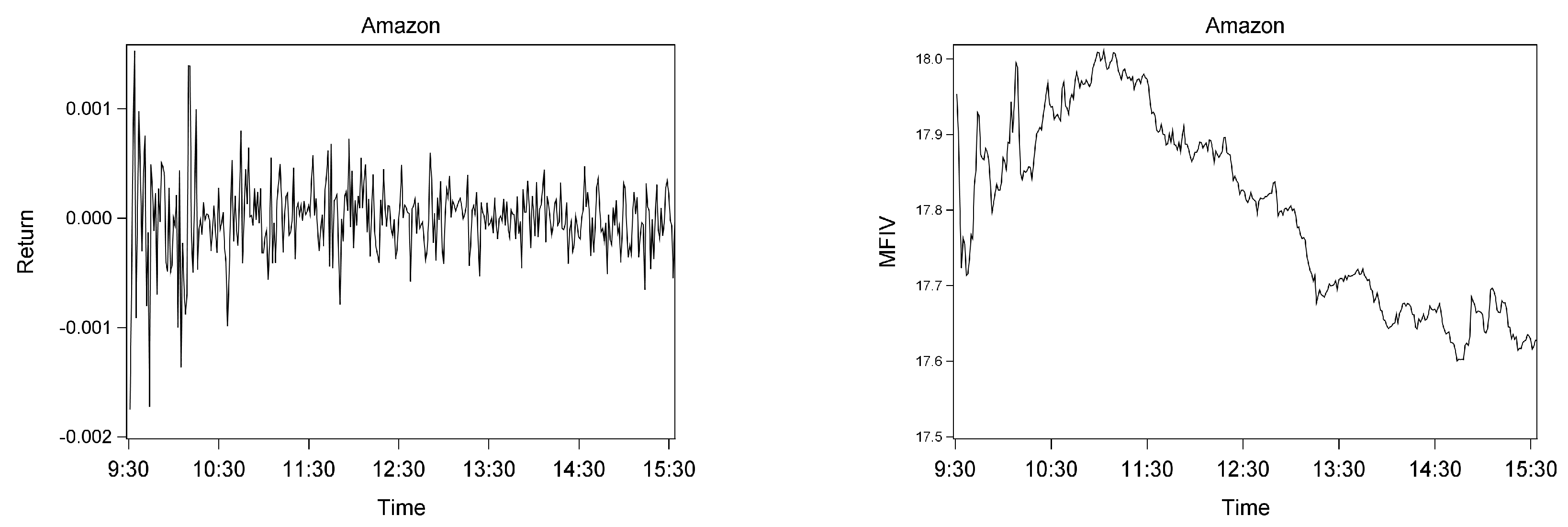
The intraday MFIV also allows us to illustrate potential diurnal patterns. Figure 2 shows the averaged MFIV over a trading day, while Figure A3 in the appendix shows the intraday (1 min) return and MFIV time series for two sample stocks on a randomly selected day. For the sample stocks and random day in Figure A3, the MFIV measures seem to capture the higher fluctuations of the intraday returns at the beginning of the trading day rather well and subsequent decreases with decreasing variability of the returns throughout the day. Averaged over trading days and sample stocks, Figure 2 shows that MFIV increases at the beginning of the trading hours and slightly decreases during the day until markets close. As noted by Chen et al. (2021), this pattern is consistent with the notion that non-trading during the overnight period increases uncertainty, while trading, to some extent, resolves uncertainty. We confirm this pattern for individual equity MFIV and also find the pattern to be similar for the different size categories (detailed results are available upon request).
4. Analyzing the Intraday Return–Volatility Relationship
The 1 min frequency of the MFIV measures allows us to examine whether specific relationships and stylized facts also hold on an intraday and individual equity level. So far, the return–volatility relationship in financial markets has been analyzed extensively. While theoretically higher risks have to be compensated by higher returns, indicating a positive relationship, empirical studies mostly document a negative and potentially asymmetric relationship between returns and changes in volatility6. Concerning equity markets, fundamental theories have been put forward to explain this negative link. The leverage hypothesis suggested by Black (1976) and Christie (1982) explains an increase in equity volatility with a decline in the value of the firm, while the volatility-feedback hypothesis associates an increase in volatility with higher expected returns and lower current prices7. As explained by Bollerslev et al. (2006), both theories differ mainly by their implied direction of causality.
More recently, Hibbert et al. (2008) (among others) proposed a behavioral perspective and associated the negative return–volatility relationship with the presence of different groups of investors. These groups may differ with respect to the extent to which they are prone to behavioral biases, such as representativeness, affect, and extrapolation biases. In contrast to the leverage and volatility-feedback hypothesis, which may take time to establish and, therefore, are more plausible at lower frequencies, behavioral biases may very well be present even at intraday frequencies. However, existing studies on the return–volatility relationship at higher frequencies are rare and have focused mostly on equity indices8. Therefore, we use our intraday MFIV measures to examine the intraday return–volatility relationship for the individual equities in our sample.
For the subsequent analysis, we show results using the WK MFIV measures and what we refer to as the feasible subset of stocks, as outlined in Section 3.2 over the range of our sampling period. The sample covers the time period from 1 May 2017 to 30 June 2017, and we conduct our analysis on 1 min, 10 min, and 60 min frequencies. Results based on the other measures are qualitatively similar and are available upon request. Despite the fact that the intraday MFIV measures exhibit only weak diurnal patterns, we conduct some basic stock-wise deseasonalization via standardization based on the time-day averages over all the sample days.
We follow Talukdar et al. (2017), Hibbert et al. (2008), Bekiros et al. (2017), and Badshah (2013) and conduct linear and quantile regressions using intraday stock-specific data on the 1, 10, and 60 min frequencies. We start with the following regressions:
where indicates the first differences of the MFIV measure for a specific underlying and represents the corresponding (positive and negative) log returns. We run our model on 1, 10, and 60 min frequencies.
Table 4 gives the regression results averaged over all sample stocks. We observe a negative average effect of contemporaneous returns (), which increases in strength with decreasing sampling frequency. The average effect of negative contemporaneous returns is slightly more pronounced compared to the one of positive returns only for the 1 min and 60 min samples. Furthermore, the number of significant negative estimates and the strength of the effect decrease with increasing lag length. These findings constitute some first evidence that the asymmetric return–volatility relationship is evident on an intraday and stock-specific level. They correspond to findings on the index level by, e.g., Talukdar et al. (2017) and Hibbert et al. (2008) in so far as the contemporaneous returns are the most important factor in determining the current changes in volatility. The results are in line with the behavioral explanations mentioned by Talukdar et al. (2017) and Hibbert et al. (2008). However, since the effects of lagged returns are not overall insignificant, leverage or volatility-feedback phenomena cannot be ruled out as well.
To account for the fact that standard regressions may not constitute an adequate approach when applied to commonly leptokurtic returns, we conduct quantile regressions following Koenker and Bassett (1978), Bekiros et al. (2017), Badshah et al. (2016), and Daigler et al. (2014):
where refers to the parameter associated with the quantile regression model equation for the qth quantile. Average results for selected quantiles are shown in Table 5 for the 1 min frequency; results for 10 and 60 min MFIV are provided in the appendix. We observe a significant negative effect of contemporaneous returns on volatility changes for the majority of our sample stocks across all quantiles. We also find this effect to vary in strength across quantiles, being more pronounced in the tails of the distribution.
Figure 3 illustrates the average coefficients over a larger range of quantiles including average confidence bounds for 1 min data (results for other frequencies are available upon request and lead to similar conclusions). The results reveal substantial variation in the effects depending on the quantiles. We observe an inverted U-shaped pattern for the contemporaneous returns, where extreme returns have a substantially stronger negative impact on current volatility compared to those in the center of the distribution. This pattern corresponds to the one detected by Agbeyegbe (2016) for the U.S. stock market indices.
Over all quantiles, contemporaneous returns are the most important factor consistent with behavioral theories, in particular, those of affect and representativeness.9 Contrary to Badshah (2013), we find no convincing evidence for loss aversion because extreme changes in the left tail do not seem to have a systematic higher impact than those in the right tail (Kahneman and Tversky 2013). Altogether, we find a significant negative contemporaneous return–volatility relationship on the intraday level for individual equity. The effect increases with decreasing sampling frequency and is more pronounced in the extreme tails of the distributions. Considering the high frequency and the insignificant or small lagged effects, it is more likely that the asymmetric relationships are caused by behavioral biases rather than the fundamental theories underlying the leverage or volatility-feedback effects.
5. Conclusions
We implement the CBOE VIX method on intraday option data for individual equities. In doing so, we analyze the data quality with respect to the MFIV calculation. Our descriptive data analysis reveals that, for 138 individual equities, weekly options exhibit a sufficient range of strike prices to avoid significant truncation errors according to Jiang and Tian (2005). Descriptive analyses of MFIV sample averages based on weekly options, monthly options, and a cubic spline interpolation approach reveal only marginal differences. We find the intraday individual equity MFIV measures to exhibit a similar diurnal pattern as implied volatility indices, such as the VIX, with higher levels after opening hours and declining levels until closing hours.
We use our estimates to analyze the intraday return volatility–relationship using 1, 10, and 60 min data. We find a negative relationship between returns and volatility changes, which is significant for most of our sample stocks when considering contemporaneous returns. The stronger the link, the lower the frequency. For lagged returns, the effect is less evident. Quantile regressions reveal a clear inverted U-shaped pattern when considering contemporaneous returns, which again becomes less evident for lagged returns. These findings indicate that behavioral biases rather than the fundamental theories of leverage or volatility-feedback effects cause the asymmetric link between returns and volatility. Despite offering a starting point for calculating and analyzing individual equity MFIV at high frequencies, our approach comes with some limitations. The standard VIX calculation method is prone to have a specific cut-off rule to determine what option quotes are used in computing the VIX. As outlined by Andersen et al. (2015), this may bias the calculated MFIV measures. Andersen et al. (2015) offered an improved approach, termed the Corridor Implied Volatility, which alleviates the potential bias of the standard measure. Moreover, Andersen et al. (2015) noted that the relationship between returns and volatility is prone to jumps and co-jumps in both series and may be more complex depending on different regimes. Subsequently, while our empirical analysis of the return–volatility relationship may offer a valid starting point, future research should be conducted accounting for a potential dynamic nature of this relationship. Overall, our individual equity MFIV measure opens up avenues for further research. The forward-looking nature of implied volatility may have merits for volatility prediction on an intraday level, as well as on a daily level for individual equities. Moreover, the derived time series of intraday MFIV measures will allow us to assess the imminent effect of news on volatility relying on time series models. They also offer the opportunity to address the impact of attention and sentiment measures at such high frequencies. It will also be of great interest to extend the sampling period throughout the pandemic period and analyze the impact of lockdown situations on the stock volatilities of different industries. In general, MFIV measures also allow a decomposition into the conditional variance of stock returns and the equity variance premium, where the latter has been shown to possess predictive power for stock returns. The proposed MFIV measures can also be used to decompose volatility into a systematic risk component and idiosyncratic risk, using the VIX index as a measure of market risk. Such idiosyncratic risk measures, then again, may yield interesting insights into investors’ risk perceptions and resulting investment decisions, potentially depending on and varying during high and low market volatility regimes.
Author Contributions
The authors contributed equally to this work. All authors have read and agreed to the published version of the manuscript.
Funding
Franziska J. Peter acknowledges funding by the German Research Foundation, Project PE 2370.
Data Availability Statement
Data sharing is not applicable.
Conflicts of Interest
The authors declare no conflicts of interest.
Appendix A. Derivation of Model-Free Implied Volatility
Following Demeterfi et al. (1999), assume the asset price S follows a continuous diffusion process:
where the drift and volatility are functions of time t and is a Brownian motion. From Ito’s lemma, we have
as shown in Appendix A. Using Equations (A1) and (A2), we can derive a representation of the incremental variance as
The realized (integrated) variance , with T denoting the time of expiration, is then given by
where and refer to the initial and final prices of the asset, respectively.
In the next step, we take risk-neutral expectations of Equation (A4):
A risk-neutral setting, using the risk-free rate r implies
The risk neutral expectation of term (1) in Equation (A5) is subsequently given by
The replication of term (2) of Equation (A5) requires a more intricate methodology. First, we decompose the logarithmic payoff by introducing the parameter , which also defines the boundary between put and call options that are used for the replication:
While term (2) here is constant, replicating term (1) is where the option methodology comes in. As Carr and Madan (1997) show in their appendix, any twice-differentiable payoff, , can be replicated as
For our setting, we use , , , the functions and to denote option prices with strike K for underlying price S and the put-call parity to write
This replication strategy relies on the availability of a continuum of strike prices. Taking the risk-neutral expectation for term (1) in Equation (A7) yields
where , , and denote the initial put, call, and underlying prices, respectively. Finally, we combine above results with Equations (A6) and (A7), and the replication of the expected variance reads as
Following Jiang and Tian (2007), it can be shown that the non-integral terms in Equation (A8) can be restated as
Applying the Taylor series expansion and ignoring terms higher than second-order yields
which results in the final approximation formula:
Ito’s Lemma for ln(St)
Applying Ito’s lemma to the natural logarithm function yields
Appendix B. Additional Figures and Tables
Figure A1.
Exemplary option dataset (AAPL) for the MN method. Each bar represents the option contracts for a specific maturity and is colored based on its use as near-term (black) or next-term (dark gray) contract. The width represents the range of offered strike prices each minute. As this range declines sharply when the near-term contract reaches maturity, the set of contracts switches 5 trading days before that date.

Figure A2.
Return series and autocorrelation functions for MFIV measures. The figure shows the stock return series over the whole sampling period at the 1 min, 10 min, and 60 min frequencies and the ACF for the MFIV measures based on weekly options for a sample stock (Amazon).
Figure A2.
Return series and autocorrelation functions for MFIV measures. The figure shows the stock return series over the whole sampling period at the 1 min, 10 min, and 60 min frequencies and the ACF for the MFIV measures based on weekly options for a sample stock (Amazon).
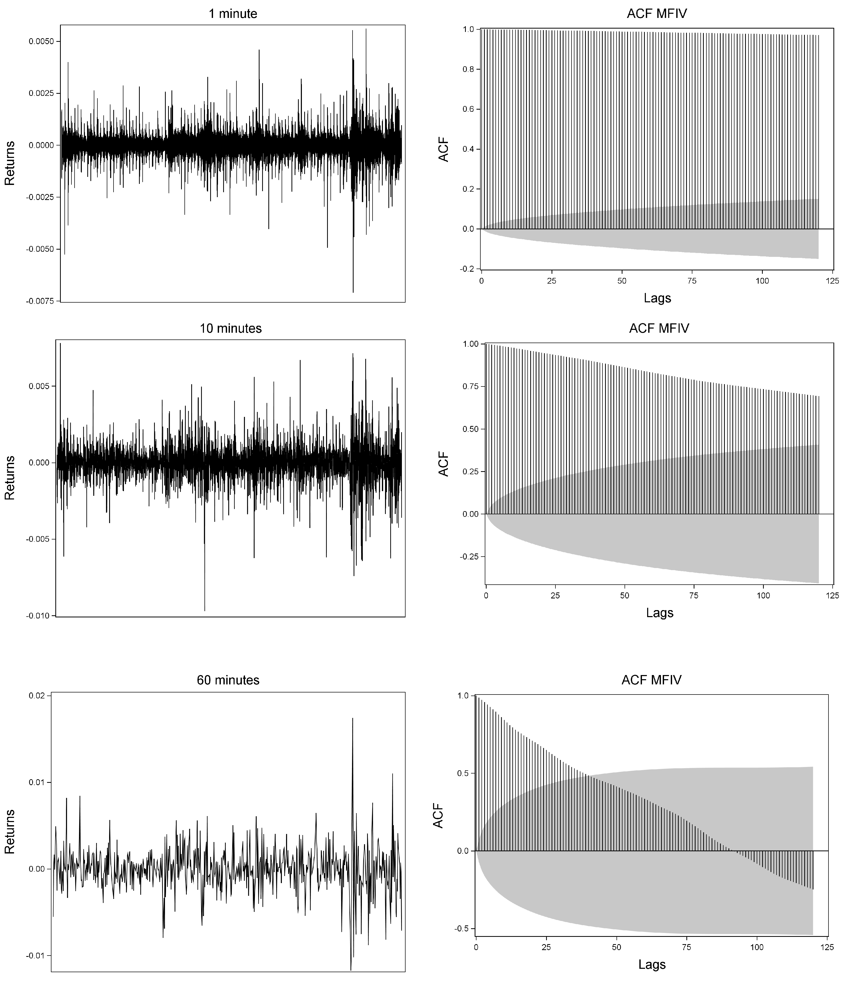
Figure A3.
MVIF measure and stock returns. The figure shows the MFIV measure time series based on weekly options for a random day and two stocks for the 1 min frequencies.
Figure A3.
MVIF measure and stock returns. The figure shows the MFIV measure time series based on weekly options for a random day and two stocks for the 1 min frequencies.


Table A1.
Average quantile regression results using 10 min data. Average quantile regression results for individual equity based on Equation (1). Average (over all sample firms) parameter estimates are reported for different quantiles. Numbers in parentheses give the numbers of significant negative/significant positive parameter estimates based on a 5% significance level.
| 0.025 | 0.05 | 0.10 | 0.25 | 0.50 | 0.75 | 0.90 | 0.95 | 0.975 | |
|---|---|---|---|---|---|---|---|---|---|
| −13.764 | −11.538 | −9.993 | −9.201 | −9.043 | −9.732 | −10.825 | −12.316 | −14.233 | |
| (104/18) | (105/17) | (110/12) | (109/13) | (109/13) | (110/11) | (108/14) | (107/15) | (104/18) | |
| −1.470 | −1.253 | −1.015 | −0.988 | −0.958 | −1.154 | −1.926 | −2.195 | −3.723 | |
| (87/35) | (92/31) | (93/28) | (93/29) | (94/28) | (97/25) | (94/28) | (94/28) | (92/30) | |
| −0.438 | −0.532 | −0.365 | −0.182 | −0.165 | −0.364 | −0.763 | −1.368 | −2.889 | |
| (79/43) | (81/41) | (77/45) | (67/55) | (71/51) | (79/43) | (88/34) | (85/37) | (93/29) | |
| −0.202 | −0.552 | −0.356 | −0.188 | −0.228 | −0.323 | −0.695 | −1.203 | −1.550 | |
| (66/56) | (78/44) | (78/44) | (77/44) | (74/44) | (70/52) | (78/44) | (80/42) | (82/40) | |
| −0.12 | −0.09 | −0.07 | −0.05 | −0.03 | −0.03 | −0.05 | −0.09 | −0.15 | |
| (101/21) | (103/19) | (105/17) | (100/22) | (91/31) | (93/29) | (94/28) | (90/32) | (85/37) | |
| −0.063 | −0.041 | −0.029 | −0.016 | −0.009 | −0.009 | −0.020 | −0.040 | −0.071 | |
| (89/33) | (91/31) | (91/31) | (90/32) | (81/41) | (75/41) | (90/32) | (84/38) | (77/45) | |
| −0.025 | −0.017 | −0.012 | −0.005 | 0.000 | 0.000 | −0.004 | −0.013 | −0.032 | |
| (89/33) | (87/35) | (83/39) | (83/39) | (79/43) | (74/48) | (81/41) | (76/46) | (74/48) | |
| constant | −0.380 | −0.227 | −0.135 | −0.056 | −0.006 | 0.038 | 0.132 | 0.268 | 0.503 |
| (122/0) | (122/0) | (122/0) | (122/0) | (108/4) | (0/122) | (0/122) | (0/122) | (0/122) |
Table A2.
Average quantile regression results using 60 min data. Average quantile regression results for individual equity based on Equation (1). Average (over all sample firms) parameter estimates are reported for different quantiles. Numbers in parentheses give the number of significant negative/significant positive parameter estimates based on a 5% significance level.
| 0.025 | 0.05 | 0.10 | 0.25 | 0.50 | 0.75 | 0.90 | 0.95 | 0.975 | |
|---|---|---|---|---|---|---|---|---|---|
| −13.764 | −11.538 | −9.993 | −9.201 | −9.043 | −9.732 | −10.825 | −12.316 | −14.233 | |
| (104/18) | (105/17) | (110/12) | (109/13) | (109/13) | (110/11) | (108/14) | (107/15) | (104/18) | |
| −1.470 | −1.253 | −1.015 | −0.988 | −0.958 | −1.154 | −1.926 | −2.195 | −3.723 | |
| (87/35) | (92/31) | (93/28) | (93/29) | (94/28) | (97/25) | (94/28) | (94/28) | (92/30) | |
| −0.438 | −0.532 | −0.365 | −0.182 | −0.165 | −0.364 | −0.763 | −1.368 | −2.889 | |
| (79/43) | (81/41) | (77/45) | (67/55) | (71/51) | (79/43) | (88/34) | (85/37) | (93/29) | |
| −0.202 | −0.552 | −0.356 | −0.188 | −0.228 | −0.323 | −0.695 | −1.203 | −1.550 | |
| (66/56) | (78/44) | (78/44) | (77/44) | (74/44) | (70/52) | (78/44) | (80/42) | (82/40) | |
| −0.12 | −0.09 | −0.07 | −0.05 | −0.03 | −0.03 | −0.05 | −0.09 | −0.15 | |
| (101/21) | (103/19) | (105/17) | (100/22) | (91/31) | (93/29) | (94/28) | (90/32) | (85/37) | |
| −0.063 | −0.041 | −0.029 | −0.016 | −0.009 | −0.009 | −0.020 | −0.040 | −0.071 | |
| (89/33) | (91/31) | (91/31) | (90/32) | (81/41) | (75/41) | (90/32) | (84/38) | (77/45) | |
| −0.025 | −0.017 | −0.012 | −0.005 | 0.000 | 0.000 | −0.004 | −0.013 | −0.032 | |
| (89/33) | (87/35) | (83/39) | (83/39) | (79/43) | (74/48) | (81/41) | (76/46) | (74/48) | |
| constant | −0.380 | −0.227 | −0.135 | −0.056 | −0.006 | 0.038 | 0.132 | 0.268 | 0.503 |
| (122/0) | (122/0) | (122/0) | (122/0) | (108/4) | (0/122) | (0/122) | (0/122) | (0/122) |
| 1 | We developed an R package for these calculations, which is currently available on https://github.com/m-g-h/R.MFIV, accessed on 20 November 2023. |
| 2 | Critically assessed, the notion of “model-freeness” is not entirely correct since an assumption about the underlying price process is still made. However, no option pricing model is required, which frees the IV from limitations due to potentially unrealistic model assumptions. |
| 3 | i.e., multiples of , with the ATM Black & Scholes IV and the time to maturity. |
| 4 | The VIX method is derived for European-style options only. Individual equity options, however, are American-style options and may be subject to an early exercise premium. As this premium can be assumed to be relatively small for out-of-the-money options and since we do not want to rely on a specific option pricing model for estimation, we do not account for it. |
| 5 | Jarque-Bera tests indicate the rejection of a normal distribution for all individual equity MFIVs. Detailed results are available upon request. |
| 6 | Compare Dennis et al. (2006), Fleming et al. (1995), Giot (2005), Hibbert et al. (2008), Carr and Wu (2017), and Talukdar et al. (2017). |
| 7 | |
| 8 | |
| 9 | Among others outlined by Hibbert et al. (2008) and Daigler et al. (2014), investors may view a high return and low risk (decreasing volatility) as representative of a good investment. Combined with an affect heuristic, where investors’ decisions may be governed or at least affected by intuition and instincts, they may act on the negative returns and high volatility, which are both negatively labeled and thereby cause a negative return–volatility relationship. |
References
- Agbeyegbe, Terence D. 2016. Modeling US stock market volatility-return dependence using conditional copula and quantile regression. Studies in Economic Theory 29: 597–621. [Google Scholar] [CrossRef]
- Andersen, Torben G., Oleg Bondarenko, and Maria T. Gonzalez-Perez. 2015. Exploring return dynamics via corridor implied volatility. The Review of Financial Studies 28: 2902–45. [Google Scholar] [CrossRef]
- Andersen, Torben G., Tim Bollerslev, Francis X. Diebold, and Heiko Ebens. 2001. The distribution of realized stockrreturn volatility. Journal of Financial Economics 61: 43–76. [Google Scholar] [CrossRef]
- Andersen, Torben, Ilya Archakov, Leon Grund, Nikolaus Hautsch, Yifan Li, Sergey Nasekin, Ingmar Nolte, Manh Cuong Pham, Stephen Taylor, and Viktor Todorov. 2021. A Descriptive Study of High-Frequency Trade and Quote Option Data*. Journal of Financial Econometrics 19: 128–77. [Google Scholar] [CrossRef]
- Badshah, Ihsan Ullah. 2013. Quantile regression analysis of the asymmetric return-volatility relation: Quantile regression analysis. Journal of Futures Markets 33: 235–65. [Google Scholar] [CrossRef]
- Badshah, Ihsan, Bart Frijns, Johan Knif, and Alireza Tourani-Rad. 2016. Asymmetries of the intraday return-volatility relation. International Review of Financial Analysis 48: 182–92. [Google Scholar] [CrossRef]
- Bekaert, Geert, and Guojun Wu. 2000. Asymmetric Volatility and Risk in Equity Markets. The Review of Financial Studies 13: 1–42. [Google Scholar] [CrossRef]
- Bekiros, Stelios, Mouna Jlassi, Kamel Naoui, and Gazi Uddin. 2017. The asymmetric relationship between returns and implied volatility: Evidence from global stock markets. Journal of Financial Stability 30: 156–74. [Google Scholar]
- Black, Fischer. 1976. Studies of Stock Market Volatility Changes. Irvine: Scientific Research Publishing Inc., pp. 177–81. [Google Scholar]
- Black, Fischer, and Myron Scholes. 1973. The pricing of options and corporate liabilities. Journal of Political Economy 81: 637–54. [Google Scholar] [CrossRef]
- Bollerslev, Tim, Julia Litvinova, and George Tauchen. 2006. Leverage and Volatility Feedback Effects in High-Frequency Data. Journal of Financial Econometrics 4: 353–84. [Google Scholar] [CrossRef]
- Breeden, Douglas T., and Robert H. Litzenberger. 1978. Prices of state-contingent claims implicit in option prices. Journal of Business 51: 621–51. [Google Scholar]
- Britten-Jones, Mark, and Anthony Neuberger. 2000. Option prices, implied price processes, and stochastic volatility. The Journal of Finance 55: 839–66. [Google Scholar] [CrossRef]
- Campbell, John Y., and Ludger Hentschel. 1992. No news is good news: An asymmetric model of changing volatility in stock returns. Journal of Financial Economics 31: 281–318. [Google Scholar] [CrossRef]
- Carr, Peter, and Dilip Madan. 1997. Towards a Theory of Volatility Trading. Cambridge: Cambridge University Press. [Google Scholar]
- Carr, Peter, and Liuren Wu. 2017. Leverage effect, volatility feedback, and self-exciting market disruptions. Journal of Financial and Quantitative Analysis 52: 2119–156. [Google Scholar] [CrossRef]
- CBOE. 2023. CBOE VIX Whitepaper. Available online: https://cdn.cboe.com/api/global/us_indices/governance/Volatility_Index_Methodology_Cboe_Volatility_Index.pdf (accessed on 20 November 2023).
- Chen, Jingjing, George J. Jiang, Chaowen Yuan, and Dongming Zhu. 2021. Breaking vix at open: Evidence of uncertainty creation and resolution. Journal of Banking & Finance 124: 106–60. [Google Scholar] [CrossRef]
- Christie, Andrew A. 1982. The stochastic behavior of common stock variances: Value, leverage and interest rate effects. Journal of Financial Economics 10: 407–32. [Google Scholar] [CrossRef]
- Cont, Rama. 2001. Empirical properties of asset returns: Stylized facts and statistical issues. Quantitative Finance 1: 223–36. [Google Scholar] [CrossRef]
- Daigler, Robert T., Ann Marie Hibbert, and Ivelina Pavlova. 2014. Examining the return–volatility relation for foreign exchange: Evidence from the euro vix. Journal of Futures Markets 34: 74–92. [Google Scholar] [CrossRef]
- Demeterfi, Kresimir, Emanuel Derman, Michael Kamal, and Joseph Zou. 1999. A guide to volatility and variance swaps. The Journal of Derivatives 6: 9–32. [Google Scholar] [CrossRef]
- Dennis, Patrick, Stewart Mayhew, and Chris Stivers. 2006. Stock returns, implied volatility innovations, and the asymmetric volatility phenomenon. Journal of Financial and Quantitative Analysis 41: 381–406. [Google Scholar] [CrossRef]
- Fleming, Jeff, Barbara Ostdiek, and Robert E. Whaley. 1995. Predicting stock market volatility: A new measure. Journal of Futures Markets 15: 265–302. [Google Scholar] [CrossRef]
- French, Kenneth R., G. William Schwert, and Robert F. Stambaugh. 1987. Expected stock returns and volatility. Journal of Financial Economics 19: 3–29. [Google Scholar] [CrossRef]
- Giot, Pierre. 2005. Relationships between implied volatility indexes and stock index returns. The Journal of Portfolio Management 31: 92–100. [Google Scholar] [CrossRef]
- Gonzalez-Perez, Maria T. 2015. Model-free volatility indexes in the financial literature: Areview. International Review of Economics & Finance 40: 141–59. [Google Scholar] [CrossRef]
- Green, Richard C., and Robert A. Jarrow. 1987. Spanning and completeness in markets with contingent claims. Journal of Economic Theory 41: 202–10. [Google Scholar] [CrossRef]
- Hibbert, Ann Marie, Robert T. Daigler, and Brice Dupoyet. 2008. A behavioral explanation for the negative asymmetric return–volatility relation. Journal of Banking & Finance 32: 2254–66. [Google Scholar] [CrossRef]
- Ishida, Isao, Michael McAleer, and Kosuke Oya. 2011. Estimating the leverage parameter of continuous-time stochastic volatility models using high frequency s&p 500 and VIX. Managerial Finance 37: 1048–67. [Google Scholar] [CrossRef]
- Jiang, George J., and Yisong S. Tian. 2005. The model-free implied volatility and its information content. The Review of Financial Studies 18: 1305–42. [Google Scholar] [CrossRef]
- Jiang, George J., and Yisong S. Tian. 2007. Extracting model-free volatility from option prices: An examination of the VIX index. The Journal of Derivatives 14: 35–60. [Google Scholar] [CrossRef]
- Kahneman, Daniel, and Amos Tversky. 2013. Prospect theory: An analysis of decision under risk. In Handbook of the Fundamentals of Financial Decision Making. Singapore: World Scientific Publishing, pp. 99–127. [Google Scholar] [CrossRef]
- Kalnina, Ilze, and Dacheng Xiu. 2017. Nonparametric estimation of the leverage effect: A trade-off between robustness and efficiency. Journal of the American Statistical Association 112: 384–96. [Google Scholar] [CrossRef]
- Koenker, Roger, and Gilbert Bassett. 1978. Regression quantiles. Econometrica 46: 33–50. [Google Scholar] [CrossRef]
- Latané, Henry A., and Richard J. Rendleman. 1976. Standard deviations of stock price ratios implied in option prices. The Journal of Finance 31: 369–81. [Google Scholar] [CrossRef]
- Nachman, David C. 1988. Spanning and completeness with options. The Review of Financial Studies 1: 311–28. [Google Scholar] [CrossRef]
- Poon, Ser-Huang, and Clive W. J. Granger. 2003. Forecasting volatility in financial markets: A review. Journal of Economic Literature 41: 478–539. [Google Scholar] [CrossRef]
- Talukdar, Bakhtear, Robert T. Daigler, and A. M. Parhizgari. 2017. Expanding the explanations for the return–volatility relation. Journal of Futures Markets 37: 689–716. [Google Scholar] [CrossRef]
- Taylor, Stephen J., Pradeep K. Yadav, and Yuanyuan Zhang. 2010. The information content of implied vlatilities and model-free volatility expectations: Evidence from options written on individual stocks. Journal of Banking & Finance 34: 871–81. [Google Scholar] [CrossRef]
- Whaley, Robert E. 1993. Derivatives on market volatility: Hedging tools long overdue. The Journal of Derivatives Fall 1: 71–84. [Google Scholar] [CrossRef]
- Whaley, Robert E. 2000. The investor fear gauge. The Journal of Portfolio Management 26: 12–17. [Google Scholar] [CrossRef]
Figure 1.
Option contracts used for the MFIV interpolation (gray) and resulting MFIV (black). Panel (a) shows the weekly option contracts used for the WK approach, which usually form a narrow corridor. Panel (b) shows the set of monthly option contracts used for the MN approach, which form a wider corridor that is sometimes “breached”.

Figure 2.
Diurnal pattern of the MFIV. The graph shows the WK, MN, and SP MFIV measures averaged over the sample stocks as well as over the sample days.
Figure 2.
Diurnal pattern of the MFIV. The graph shows the WK, MN, and SP MFIV measures averaged over the sample stocks as well as over the sample days.

Figure 3.
Quantile regression estimates and confidence intervals. The plots show the average estimated parameters based on Equation (1) for different quantiles (solid line) together with their 0.95 confidence bounds.
Figure 3.
Quantile regression estimates and confidence intervals. The plots show the average estimated parameters based on Equation (1) for different quantiles (solid line) together with their 0.95 confidence bounds.
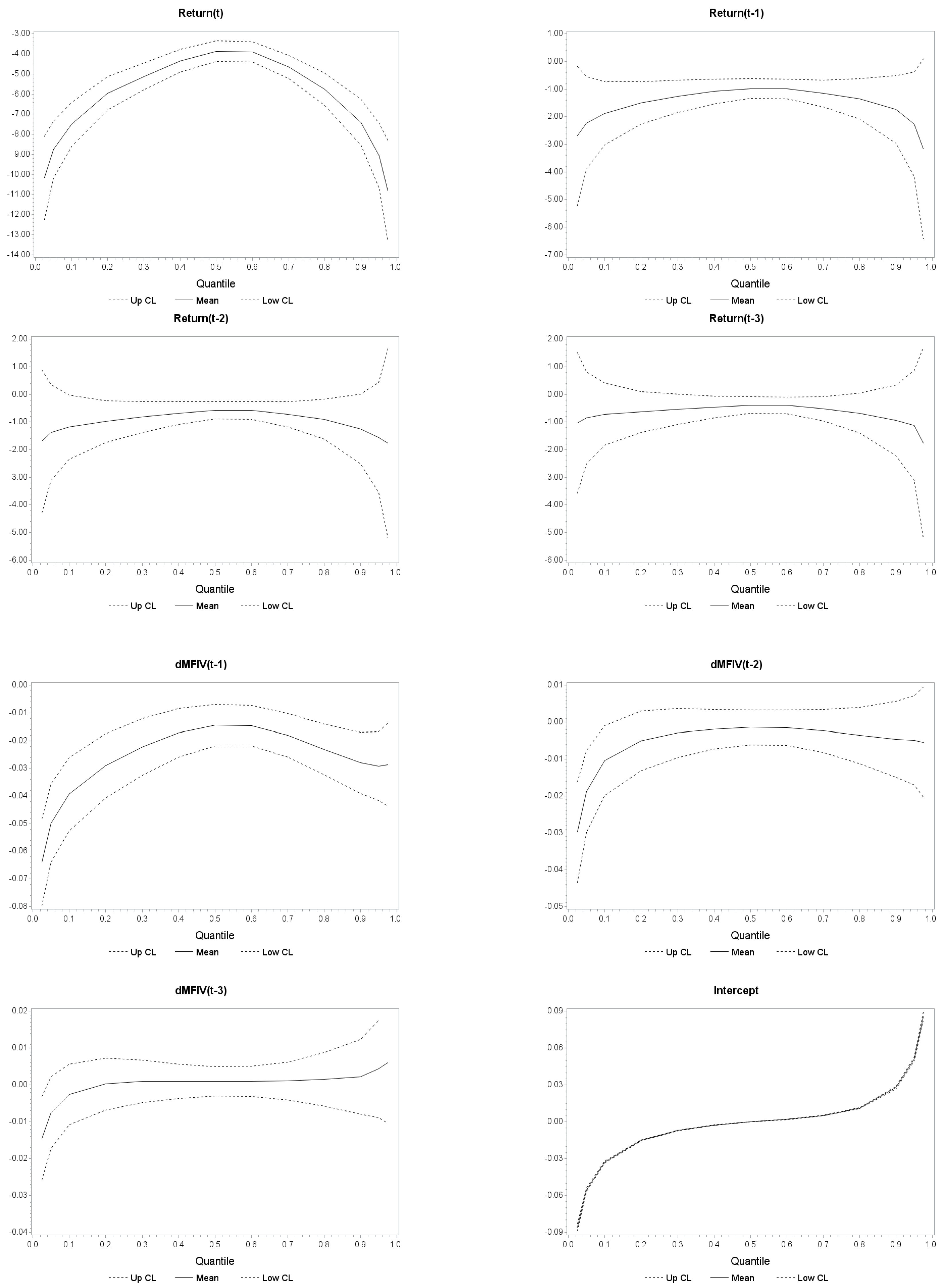
Table 1.
Descriptive statistics. The table groups the stocks by their market capitalization (, quoted in million USD). The average number of call and put options is given by and . The average range above () and below () the current ATM forward price , as well as the average spacing of the strikes (), are measured in standard deviations of price. We also report the average price (P), return (R), standard deviation of return (), and MFIV. The number of stocks is given by n, and “Set” refers to the set of options for the respective interpolation approach.
| Size | MC | Calls | Puts | Max K | Min K | dK | n | P | R | R (sd) | MFIV |
|---|---|---|---|---|---|---|---|---|---|---|---|
| WK Set | |||||||||||
| Any | 101,337 | 11.0 | 13.8 | 1.75 | 2.31 | 0.274 | 178 | 104.37 | 0.0008 | 26.82 | |
| Mega | 485,985 | 11.4 | 18.1 | 1.93 | 3.11 | 0.337 | 21 | 205.50 | 0.0005 | 17.84 | |
| Large | 65,180 | 11.2 | 14.0 | 1.77 | 2.34 | 0.275 | 117 | 105.33 | 0.0008 | 25.08 | |
| Medium | 5692 | 10.0 | 11.0 | 1.61 | 1.82 | 0.237 | 33 | 51.52 | 0.0010 | 36.38 | |
| Small | 1359 | 10.8 | 9.8 | 1.65 | 1.67 | 0.238 | 7 | 34.04 | 0.0012 | 37.73 | |
| MN Set | |||||||||||
| Any | 101,337 | 8.2 | 10.1 | 2.06 | 2.74 | 0.436 | 178 | 104.37 | 0.0008 | 27.02 | |
| Mega | 485,985 | 9.1 | 14.4 | 2.30 | 3.84 | 0.539 | 21 | 205.50 | 0.0005 | 18.15 | |
| Large | 65,180 | 8.1 | 9.9 | 2.06 | 2.78 | 0.447 | 117 | 105.33 | 0.0008 | 25.34 | |
| Medium | 5692 | 8.0 | 8.4 | 1.93 | 2.11 | 0.344 | 33 | 51.52 | 0.0010 | 36.40 | |
| Small | 1359 | 8.1 | 6.7 | 1.92 | 1.84 | 0.374 | 7 | 34.04 | 0.0012 | 37.50 | |
| SP Set | |||||||||||
| Any | 101,337 | 9.0 | 11.8 | 3.27 | 3.80 | 0.349 | 178 | 104.37 | 0.0008 | 26.97 | |
| Mega | 485,985 | 9.6 | 16.4 | 3.86 | 5.34 | 0.407 | 21 | 205.50 | 0.0005 | 18.05 | |
| Large | 65,180 | 8.8 | 11.8 | 3.28 | 3.90 | 0.357 | 117 | 105.33 | 0.0008 | 25.28 | |
| Medium | 5692 | 9.2 | 9.8 | 2.90 | 2.74 | 0.290 | 33 | 51.52 | 0.0010 | 36.39 | |
| Small | 1359 | 7.5 | 3.02 | 2.43 | 0.321 | 7 | 34.04 | 0.0012 | 37.51 | ||
Table 2.
Descriptives on MFIV measures. The table presents descriptive statistics on MFIV measures based on monthly options (MN), weekly options (WK), and the interpolation approach (SP) for all samples and the small, medium, large, and mega cap sample firms.
Table 2.
Descriptives on MFIV measures. The table presents descriptive statistics on MFIV measures based on monthly options (MN), weekly options (WK), and the interpolation approach (SP) for all samples and the small, medium, large, and mega cap sample firms.
| Mean | Std. Dev. | Min | Max | Skewness | Kurtosis | |
|---|---|---|---|---|---|---|
| All | ||||||
| MFIV (MN) | 25.33 | 9.59 | 9.02 | 88.94 | 1.57 | 3.19 |
| MFIV (WK) | 25.03 | 9.74 | 9.71 | 86.82 | 1.58 | 3.33 |
| MFIV (SP) | 25.26 | 9.65 | 8.23 | 92.18 | 1.57 | 3.19 |
| Mega | ||||||
| MFIV (MN) | 22.50 | 7.35 | 9.02 | 88.94 | 2.27 | 9.18 |
| MFIV (WK) | 22.17 | 7.51 | 9.71 | 82.78 | 2.27 | 9.06 |
| MFIV (SP) | 22.42 | 7.38 | 8.23 | 92.18 | 2.24 | 8.95 |
| Large | ||||||
| MFIV (MN) | 33.00 | 7.37 | 13.88 | 68.63 | 0.63 | 0.58 |
| MFIV (WK) | 32.71 | 7.13 | 14.33 | 74.64 | 0.68 | 1.02 |
| MFIV (SP) | 32.95 | 7.45 | 17.60 | 65.08 | 0.73 | 0.88 |
| Medium | ||||||
| MFIV (MN) | 43.82 | 12.13 | 20.86 | 86.57 | 0.08 | −0.91 |
| MFIV (WK) | 43.93 | 12.43 | 21.44 | 86.82 | 0.17 | −0.75 |
| MFIV (SP) | 43.89 | 12.21 | 21.63 | 87.26 | 0.09 | −0.91 |
| Small | ||||||
| MFIV (MN) | 36.82 | 5.27 | 29.26 | 60.25 | 0.96 | 0.33 |
| MFIV (WK) | 37.77 | 5.76 | 26.28 | 57.44 | 0.53 | −0.93 |
| MFIV (SP) | 36.67 | 5.38 | 27.79 | 64.36 | 1.19 | 1.37 |
Table 3.
Skewness, kurtosis, and correlations of MFIV measures. The table shows the skewness and kurtosis of MFIV measures based on weekly options as well as their correlation with stock returns based on 1 min, 10 min, and 60 min frequencies.
Table 3.
Skewness, kurtosis, and correlations of MFIV measures. The table shows the skewness and kurtosis of MFIV measures based on weekly options as well as their correlation with stock returns based on 1 min, 10 min, and 60 min frequencies.
| Skewness | Kurtosis | Corr(MFIV, R) | |||||||
|---|---|---|---|---|---|---|---|---|---|
| 1 min | 10 min | 60 min | 1 min | 10 min | 60 min | 1 min | 10 min | 60 min | |
| All | 0.61 | 0.61 | 0.62 | −0.26 | −0.25 | −0.14 | 0.000 | −0.002 | −0.006 |
| Mega | 0.6 | 0.6 | 0.6 | −0.27 | −0.28 | −0.21 | 0.000 | 0.001 | 0.001 |
| Large | 0.62 | 0.63 | 0.68 | −0.3 | −0.21 | 0.15 | −0.001 | −0.014 | −0.037 |
| Medium | 0.68 | 0.68 | 0.69 | 0.18 | 0.16 | 0.17 | −0.001 | −0.004 | −0.016 |
| Small | 0.54 | 0.55 | 0.56 | −0.72 | −0.71 | −0.6 | −0.003 | −0.007 | −0.027 |
Table 4.
Average return–volatility regression results. Regression Results for 1, 10, and 60 min frequencies averaged over the sample stocks. The parameters indicate the effect of positive returns (), negative returns (), and first differences in MFIV () on the first differences in MFIV for lags L of 0 to 3. Numbers in parentheses give the amount of significant negative/significant positive parameter estimates based on a 5% significance level.
| 1 min | 10 min | 60 min | |
|---|---|---|---|
| −7.69 | −14.79 | −15.17 | |
| (66/1) | (65/14) | (69/15) | |
| −1.22 | −1.98 | −2.27 | |
| (25/5) | (52/9) | (31/7) | |
| −1.22 | −1.26 | −1.58 | |
| (24/1) | (28/6) | (25/4) | |
| −0.89 | −0.23 | −1.35 | |
| (21/2) | (12/5) | (20/5) | |
| −9.01 | −13.17 | −15.35 | |
| (81/1) | (74/14) | (74/14) | |
| −5.03 | −4.31 | −4.22 | |
| (52/1) | (47/10) | (42/4) | |
| −2.95 | −2.41 | −3.02 | |
| (35/2) | (32/8) | (24/7) | |
| −2.48 | −1.53 | −2.37 | |
| (16/3) | (21/6) | (19/6) | |
| −0.12 | −0.15 | −0.13 | |
| (88/0) | (92/0) | (64/0) | |
| −0.07 | −0.06 | −0.05 | |
| (55/2) | (53/1) | (37/1) | |
| −0.03 | −0.02 | −0.03 | |
| (31/2) | (22/0) | (26/2) | |
| 0.00 | 0.00 | −0.01 | |
| (14/25) | (39/26) | (38/30) | |
| 16 | 60 | 60 | |
| 19 | 38 | 26 |
Table 5.
Average quantile regression results using 1 min data Average quantile regression results for individual equity based on Equation (1). Average (over all sample firms) parameter estimates are reported for different quantiles. Numbers in parentheses give the amount of significant negative/significant positive parameter estimates based on a 5% significance level.
| 0.025 | 0.05 | 0.10 | 0.25 | 0.50 | 0.75 | 0.90 | 0.95 | 0.975 | |
|---|---|---|---|---|---|---|---|---|---|
| −10.167 | −8.763 | −7.496 | −5.528 | −3.860 | −5.190 | −7.405 | −9.082 | −10.822 | |
| (112/2) | (110/3) | (108/4) | (103/8) | (95/5) | (100/8) | (104/5) | (107/2) | (106/3) | |
| −2.695 | −2.222 | −1.880 | −1.361 | −0.979 | −1.260 | −1.735 | −2.275 | −3.166 | |
| (67/3) | (73/3) | (83/5) | (82/5) | (80/5) | (72/5) | (73/6) | (69/4) | ( 64/4) | |
| −1.692 | −1.379 | −1.181 | −0.887 | −0.574 | −0.804 | −1.245 | −1.557 | −1.759 | |
| (50/4) | (54/1) | (64/0) | (73/0) | (79/1) | (66/1) | (60/1) | (52/2) | ( 43/5) | |
| −1.033 | −0.850 | −0.711 | −0.598 | −0.381 | −0.594 | −0.939 | −1.115 | −1.756 | |
| (32/4) | (36/0) | (39/0) | (52/1) | (56/1) | (57/2) | (45/1) | (42/4) | ( 39/3) | |
| −0.06 | −0.05 | −0.04 | −0.03 | −0.01 | −0.02 | −0.03 | −0.03 | −0.03 | |
| (108/4) | (107/1) | (111/1) | (104/0) | (90/0) | (88/0) | (86/5) | (83/10) | (72/19) | |
| −0.030 | −0.019 | −0.010 | −0.004 | −0.001 | −0.003 | −0.005 | −0.005 | −0.005 | |
| (95/13) | (81/13) | (70/13) | (42/10) | (21/5) | (36/7) | (41/24) | (46/29) | (46/33) | |
| −0.014 | −0.008 | −0.003 | 0.001 | 0.001 | 0.001 | 0.002 | 0.004 | 0.006 | |
| (68/17) | (60/21) | (23/48) | (18/20) | (7/11) | (10/11) | (13/23) | (16/35) | (25/43) | |
| constant | −0.783 | −0.527 | −0.331 | −0.162 | −0.037 | 0.091 | 0.347 | 0.608 | 0.910 |
| (122/0) | (121/0) | (122/0) | (120/0) | (61/47) | (0/122) | (0/122) | (0/122) | (0/122) |
Disclaimer/Publisher’s Note: The statements, opinions and data contained in all publications are solely those of the individual author(s) and contributor(s) and not of MDPI and/or the editor(s). MDPI and/or the editor(s) disclaim responsibility for any injury to people or property resulting from any ideas, methods, instructions or products referred to in the content. |
© 2024 by the authors. Licensee MDPI, Basel, Switzerland. This article is an open access article distributed under the terms and conditions of the Creative Commons Attribution (CC BY) license (https://creativecommons.org/licenses/by/4.0/).
Share and Cite
MDPI and ACS Style
Haas, M.G.; Peter, F.J. Implementing Intraday Model-Free Implied Volatility for Individual Equities to Analyze the Return–Volatility Relationship. J. Risk Financial Manag. 2024, 17, 39. https://doi.org/10.3390/jrfm17010039
AMA Style
Haas MG, Peter FJ. Implementing Intraday Model-Free Implied Volatility for Individual Equities to Analyze the Return–Volatility Relationship. Journal of Risk and Financial Management. 2024; 17(1):39. https://doi.org/10.3390/jrfm17010039
Chicago/Turabian StyleHaas, Martin G., and Franziska J. Peter. 2024. "Implementing Intraday Model-Free Implied Volatility for Individual Equities to Analyze the Return–Volatility Relationship" Journal of Risk and Financial Management 17, no. 1: 39. https://doi.org/10.3390/jrfm17010039