Estimating Asset Parameters Using Levy’s Moment Matching Method

Abstract

Conventionally, the unknown parameters in Merton’s model are set using a calibration method that estimates the current asset value and volatility from observable stock prices. This paper describes a completely different approach for estimating these asset parameters. The proposed approach uses Levy’s moment matching method to derive an equation for the asset value based on the sum of equity and debt on the balance sheet, with the current debt value treated as an unknown and estimated from stock prices. Empirical analysis reveals that this method results in simpler calculations than the calibration method and can estimate the asset parameters and default probability to the same degree of accuracy. An additional advantage of the proposed method is that it estimates the asset correlation if the current debt value is known, allowing Merton’s model to be extended to multiple companies. The asset correlation obtained by the proposed method is estimated from multiple parameters related to equity, debt, and the evaluation period, which is useful when the influence of equity volatility, leverage, and time must be considered in estimating asset correlations based on equity correlations.

1. Introduction

Merton’s model, in which Merton (1974) applied the option pricing model of Black and Scholes (1973) to corporate debt value, is well known as a pioneering structured approach. The advantage of Merton’s model is that it succinctly expresses the relationship between a company’s equity and debt. Thus, given the observable stock market value, the unobservable debt market value and credit risk can be easily calculated. Therefore, the model has had a tremendous impact on subsequent academic and practical studies. One well-known example is the theory of optimal capital structure for corporate finance. Leland (1994) and Leland and Toft (1996) extended Merton’s model to solve capital structure optimization problems in situations where the Modigliani–Miller (MM) theorem does not hold. Merton’s model has also had a significant impact on credit risk management practice in banks because it allows credit risk to be estimated in addition to corporate debt value. JP Morgan’s Credit Metrics (Gupton et al. 1997) and the KMV model (Vasicek 1984) are typical examples. Merton’s model incorporates several challenging scenarios because it applies the classical Black–Scholes model. Therefore, a number of improved models have been proposed over the past half-century.

For example, Black and Cox (1976) and Briys and de Varenne (1997) relaxed the assumptions of Merton’s (1973) model, leading to first-passage-type models in which default occurs when a company’s profit reaches a certain lower threshold value. Conversely, Longstaff and Schwartz (1995) employed a stochastic process and determined that a company defaults when its asset values fail to reach a certain threshold. They expanded the Black and Cox (1976) model by incorporating a probability fluctuation model that accounts for interest rate uncertainty. Moreover, Leland (1994) and Leland and Toft (1996) considered the interest between shareholders and creditors in a corporate finance framework and determined the asset values in terms of maximizing shareholder value. Other studies include that of Geske (1977), who assumed that shareholders have the options of allotting the amortization fund of a company through the issuance of additional stocks or letting a company become bankrupt. This approach considers the possibility of additional finance. Furthermore, Collin-Dufresne and Goldstein (2001) extended the results of Longstaff and Schwartz (1995) by assuming that companies should maintain their optimal financial leverage. Scott (1981) proposed an approach for estimating the probability of default (PD) using option pricing theory, whereas Kealhofer (1993) and Vasicek (1984) estimated the PD using what is now known as the KMV model. There are many examples of companies suddenly failing despite being considered healthy (e.g., Enron, WorldCom). A mathematical point regarding the structural approach concerns whether the default time can theoretically be predicted. In other words, is there some aspect of the model that allows investors to predict the bankruptcy of companies in advance? If this were the case, the model could not account for unexpected risk. To resolve this issue, two extensions of Merton’s model have been studied. In the first, Zhou (1997, 2011) proposed a model that considers the sudden default risk by expressing the asset value of a company using jump-diffusion processes. In the second approach, Duffie and Lando (2001) and Giesecke (2003) assumed that the financial information disclosed by a company contains noise, preventing ordinary investors from determining the true value of the company. They proposed models that consider uncertainties such as instances of accounting fraud.

As the above discussion shows, many extensions of traditional models have been proposed. However, there has been insufficient analysis based on real-world examples. One reason is that the model parameters are often difficult to determine. For example, asset values cannot be obtained directly, so some theoretical approach must be applied to implicitly estimate the asset parameters from stock price data. In estimating deposit insurance premiums, Marcus and Shaked (1984) and Ronn and Verma (1989) proposed calibration methods for estimating unknown parameters such as the current asset value, asset volatility, and deposit insurance value from stock prices. They performed the estimations using two or three nonlinear equations with parameters related to equity, debt, and the evaluation period. Duan (1994) and Vassalou and Xing (2004) proposed estimation methods that determine the unknown parameters using likelihood estimation based on the option model. In contrast, the method proposed in this paper estimates the asset parameters in a completely different way, although the stock prices are still used in the estimation process. The proposed method evaluates a company’s asset value as a portfolio of equity and debt based on the balance sheet. For this, we derive an equation using Levy’s (1992) moment matching method. The current debt value, which is a parameter of this equation, is treated as an unknown and estimated from stock prices. Once the current debt value is known, the asset correlation can be estimated in addition to the current asset value and volatility. This enables Merton’s model to be extended to multiple companies.

The remainder of this paper is organized as follows: Section 2 introduces Merton’s model and the existing calibration method for estimating asset parameters. Section 3 describes the proposed alternative for estimating asset parameters. In addition, we clarify the difference between the calculation procedures of the proposed method and the calibration method using specific numerical examples. Section 4 presents the results of empirical analysis using the methods discussed in Section 2 and Section 3. In particular, we show that the asset parameters and PD obtained by the proposed method are in good agreement with those given by the calibration method. Section 5 develops a new technique for estimating the asset correlation using the proposed method and extends Merton’s model to multiple companies. Section 6 gives the results of empirical analysis using the asset correlation method, where the asset correlation is estimated from multiple parameters related to equity, debt, and the evaluation period. We also clarify how these parameters affect the estimation of asset correlation. Finally, the conclusions of this study are summarized in Section 7.

2. Merton’s Model and Existing Asset Parameter Estimation Method

In Merton’s model, the credit model is derived using an option approach. Consider a simple case in which the capital structure consists of one kind of debt that is free from interest payments and one kind of equity that pays no dividends. In this case, company bankruptcy can be defined by excess; in other words, the market value of assets at maturity is less than the value of debt to be paid off. Hence, if the distribution of asset value at maturity is specified, the PD can be estimated. Assume that the asset value $A_i\left(t\right) (0\le t\le T)$ of the i-th company obeys a geometric Brownian motion process:

$$d{A}_i\left(t\right)=r{A}_i\left(t\right)dt+{\sigma }_{A,i}{A}_i\left(t\right)d{W}_{A,i}\left(t\right),$$

(1)

where r is the risk-free rate, ${\sigma }_{A,i}$ is the asset volatility, and $W_{A,i}\left(t\right)$ follows a standard Brownian motion. From (1), the asset value $A_i\left(T\right)$ can be expressed using the current asset value $A_i\left(0\right)$:

$$A_i(T)=A_i\left(0\right)\mathit{exp}((r-{\sigma }_{A,i}^2/2)T+{\sigma }_{A,i}{W}_{A,i}(T)),$$

(2)

where $W_{A,i}\left(T\right)~N(0,T)$. Denoting the face value of the company’s debt as $F_i$, the default event can be expressed as $\left\{A_i\right(T)\le F_i\}$. At time T, Merton’s model gives the following PD:

$$\begin{array}{ll}\mathrm{Pr}\left(A_i\left(T\right)\le F_i\right)& =\mathrm{Pr}\left(\mathit{ln}{A}_i\left(T\right)\le \mathit{ln}{F}_i\right)\\ & ={\int }_{-\infty }^{\mathit{ln}{F}_i}f\left(\mathit{ln}{A}_i\left(T\right)\right)d\mathit{ln}{A}_i\left(T\right)\\ & =N\left(d_i\right),\end{array}$$

(3)

where $d_i=\frac{\mathit{ln}(F_i/A_i\left(0\right))-(r-{\sigma }_{A,i}^2/2)T}{{\sigma }_{A,i}\sqrt{T}}$, $f(\cdot )$ is the probability density function of the normal distribution, and $N(\cdot )$ is the cumulative probability density of the standard normal distribution. In this case, PD is easy to calculate from (3), but this equation cannot be directly applied to real data because it is difficult to set the model parameters. As the asset value itself cannot be observed, various methods for estimating asset parameters such as the current asset value and volatility have been developed. This section introduces the most popular estimation method, namely the calibration method. Although it is difficult to obtain the current asset value $A_i\left(0\right)$ and asset volatility ${\sigma }_{A,i}$ directly, the company’s equity value can easily be determined by multiplying the daily stock market price by the total volume of stock issued. Therefore, the unknown parameters $A_i\left(0\right)$ and ${\sigma }_{A,i}$ can be determined from nonlinear Equations (4) and (6), which relate to the equity parameters $S_i\left(0\right)$ and ${\sigma }_{s,i}$. Equation (4) expresses the relationship between the volatility of an asset and equity. From $\mathrm{It}\widehat{\mathrm{o}}$’s lemma,

$${\sigma }_{s,i}{S}_i\left(0\right)=N\left(d_i+{\sigma }_{A,i}\sqrt{T}\right){\sigma }_{A,i}{A}_i\left(0\right),$$

(4)

where $d_i$ is defined in (3), $S_i\left(0\right)$ is the current equity value, and ${\sigma }_{s,i}$ is the equity volatility. The initial value is given by

$$\underset{T\to 0}{lim}{\sigma }_{A,i}\approx \left(\frac{S_i\left(0\right)}{A_i\left(0\right)}\right){\sigma }_{s,i}.$$

(5)

Equation (6) expresses the equity value using the form of European call options. That is, at the time of debt maturity T, the equity value is given by subtracting the face value of debt $F_i$ from the asset value $A_i\left(T\right)$. Moreover, the equity value cannot become negative, even if default occurs. Thus, the current equity value $S_i\left(0\right)$ is expressed as follows:

$$\begin{array}{ll}{S}_i\left(0\right)& =e^{-rT}{E}^{*}\left[\max \left(A_i\left(T\right)-F_i,0\right)\right]\\ & =e^{-rT}{\int }_{F_i}^{\infty }\left(A_i\left(T\right)-F_i\right)F\left(A_i\left(T\right)\right)d{A}_i\left(T\right)\\ & =A_i\left(0\right)N\left(-d_i\right)-F_i{e}^{-rT}N\left(-d_i-{\sigma }_{A,i}\sqrt{T}\right),\end{array}$$

(6)

where $F(\cdot )$ is the probability density function of the lognormal distribution and $E^{*}$ is the conditional expectation with respect to risk-neutral probability. Finally, the calibration method estimates the asset parameters $A_i\left(0\right)$ and ${\sigma }_{A,i}$ from multiple parameters related to equity, debt, and the evaluation period using (4) and (6). Merton’s model applies the Black–Scholes model using the no-arbitrage condition between the company’s assets, debt, and equity and makes several strong assumptions in its application. These assumptions are that the volatility and risk-free interest rate remain constant over time and that the values of assets and equity follow a geometric Brownian motion and fluctuate continuously without large jumps. However, these assumptions are not appropriate in real markets, requiring academic and practical studies to use stochastic volatility models or models that account for jumps.

3. Alternative Asset Parameter Estimation Method

We propose an alternative method for estimating the asset parameters. The proposed estimation method, similar to the calibration method discussed in Section 2, uses stock prices to estimate unknown parameters such as the current asset value and volatility. However, the calculation procedure is very different. First, an equation for evaluating a company’s asset value is derived by considering a portfolio of equity and debt, as on a balance sheet, using Levy’s moment matching method. The current debt value, which is a parameter of this equation, is then treated as an unknown and estimated from stock prices. Our motivation for using the moment matching method in evaluating asset values is as follows: The moment matching method was originally used as an approximate method for averaging a basket of options, where the payoffs are determined by the average value and portfolio value of assets. The point of Levy’s moment matching method is that random variables with similar characteristics, such as the average value and portfolio value of assets whose true distribution is unknown, are each assumed to follow a lognormal distribution. As the asset values based on Merton’s model are the sum of equity and debt, they have similar characteristics to the average value and portfolio value of assets and are assumed to follow a lognormal distribution. This is our rationale for using the moment matching method to evaluate asset values based on Merton’s model.

To derive an equation for evaluating asset values, we first consider the asset portfolio expressing the capital structure of a company. In reality, asset portfolios are rarely simple because the accounts payable, loans, and corporate bonds related to financial affairs are all included in debt and have different maturities. Moreover, once a default occurs, the priority of various financial items must be considered. Thus, it is not advisable to examine each case. As stated in Section 2, we consider a case similar to Merton’s model in which the asset portfolio comprises one kind of debt and one kind of equity paying no dividends. The equity value is easily determined by multiplying the daily stock price by the total volume of stock issued. Assuming that equity value i (i.e., the equity of the i-th company) exhibits geometric Brownian motion, equity value $S_i\left(T\right)$ at time T is expressed in terms of $S_i\left(0\right)$ as follows:

$$S_i(T)=S_i(0)\mathit{exp}(({\mu }_{s,i}-{\sigma }_{s,i}^2/2)T+{\sigma }_{s,i}{W}_{s,i}(T)),$$

(7)

where ${\mu }_{s,i}$ is the expected return ratio of equity i and ${\sigma }_{s,i}$ is the volatility of equity i. Conversely, the debt value is not easily comparable to the equity value, and it is difficult to measure its distribution. For convenience, the debt value of the i-th company is given by $D_i(T)=D_i(0)\mathit{exp}({\mu }_{d,i}T)$ at time T; therefore, the asset portfolio $A_i(T)$ is expressed as follows:

$$\begin{array}{ll}{A}_i\left(T\right)& =S_i\left(T\right)+D_i\left(T\right)\\ & =S_i(0)\mathit{exp}(({\mu }_{s,i}-{\sigma }_{s,i}^2/2)T+{\sigma }_{s,i}{W}_{s,i}(T))+D_i(0)\mathit{exp}({\mu }_{d,i}T).\end{array}$$

(8)

Here, applying the moment matching method, we assume that another variable $X_i\left(t\right)(0\le t\le T)$ of the i-th company exhibits geometric Brownian motion with respect to the first and second moments of the asset portfolio in (8) and consider this variable to represent the asset value of the company. Under this condition, the asset value $X_i(T)$ at time T can be expressed in terms of $X_i(0)$ as follows (see Appendix A):

$$X_i(T)=X_i(0)\mathit{exp}(({\mu }_{x,i}-{\sigma }_{x,i}^2/2)T+{\sigma }_{x,i}{W}_{x,i}(T)),$$

(9)

where ${\mu }_{x,i}$ is the expected return ratio of asset i and ${\sigma }_{x,i}$ is the volatility of asset i.

$$\begin{array}{ll}{\mu }_{x,i}& =\frac{1}{T}\mathit{ln}\left[\frac{S_i(0)e^{{\mu }_{s,i}T}+D_i(0)e^{{\mu }_{d,i}T}}{X_i(0)}\right],\\ {\sigma }_{x,i}& =\sqrt{\frac{1}{T}\mathit{ln}\left[\frac{S_i(0{)}^2{e}^{(2{\mu }_{s,i}+{\sigma }_{s,i}^2)T}+2S_i(0)D_i(0)e^{({\mu }_{s,i}+{\mu }_{d,i})T}+D_i(0{)}^2{e}^{2{\mu }_{d,i}T}}{X_i(0{)}^2}\right]-2{\mu }_{x,i}}\end{array}$$

(10)

The current asset value $X_i\left(0\right)$ has the form $X_i\left(0\right)=S_i\left(0\right)+D_i\left(0\right)$. Here, substituting 0 for $D_i\left(0\right)$ in (9) gives the equity value in (7) because ${\mu }_{x,i}$ and ${\sigma }_{x,i}$ in (10) become ${\mu }_{s,i}$ and ${\sigma }_{s,i}$, respectively; furthermore, $X_i\left(0\right)=S_i\left(0\right)$. If we instead substitute 0 for $S_i\left(0\right)$ in (9), we obtain $D_i(0)\mathit{exp}({\mu }_{d,i}T)$. In this way, (9) successfully expresses the asset value when a company is unleveraged and when it is leveraged. Moreover, focusing on the evaluation period T of the parameters in (10), the expected return rate and volatility of an asset at the initial time in (10) are given by

$$\underset{T\to 0}{lim}{\mu }_{x,i}\approx \frac{S_i\left(0\right)}{X_i\left(0\right)}{\mu }_{s,i}+\frac{D_i\left(0\right)}{X_i\left(0\right)}{\mu }_{d,i},\hspace{1em}\underset{T\to 0}{lim}{\sigma }_{x,i}\approx \frac{S_i\left(0\right)}{X_i\left(0\right)}{\sigma }_{s,i}.$$

(11)

The expected return rate of an asset in (11) at the initial time is defined as the weighted average of the expected rates of return of both equity and debt. Thus, from the perspective of a company, ${\mu }_{x,i}$ in (10) can be considered as the weighted average cost of capital depending on time T. Turning to the real world, the expected rate of return of equity may be obtained from the Capital Asset Pricing Model (CAPM) or Arbitrage Pricing Theory (APT), and the expected rate of return of debt may be obtained from the ratio of interest expenses to the interest-bearing liability or bond yield. Duffie and Singleton (2003) and Berg (2010) discussed such real-world assumptions in detail. In this paper, we consider PD in a risk-neutral world, as treated in Merton’s model. Here, the expected rate of return of equity and debt in (10) is ${\mu }_{s,i}={\mu }_{d,i}=r$. Finally, the asset value of (9) can be expressed as follows:

$$X_i(T)=X_i(0)\mathit{exp}((r-{\sigma }_{x,i}^2/2)T+{\sigma }_{x,i}{W}_{x,i}(T)),$$

(12)

where

$${\sigma }_{x,i}=\sqrt{\frac{1}{T}\mathit{ln}\left[\frac{S_i(0{)}^2{e}^{\left(2r+{\sigma }_{s,i}^2\right)T}+2S_i(0)D_i(0)e^{2rT}+D_i(0{)}^2{e}^{2rT}}{X_i(0{)}^2}\right]-2r},$$

(13)

in which ${\sigma }_{x,i}$ is calculated from multiple parameters related to equity, debt, and the evaluation period. The problem concerns how to set $D_i\left(0\right)$, because the debt value itself cannot be obtained from the market in the manner of a daily stock price. Miyake and Inoue (2009) used the annual book value of $D_i\left(0\right)$ as the current debt value, but this is incorrect from the viewpoint of risk. Because other companies typically have a greater or lesser possibility of default, the debt value should be treated as an uncertain item together with the default risk. Namely, the realistic debt value must be lower than the book value. Otherwise, when estimating the asset parameters, the current asset value would be higher and the asset volatility would be lower, leading to the underestimation of PD. The proposed approach improves this situation by introducing the default risk into the debt value. Let the face value of a loan at the maturity date be F. Then, the following expression is a form of the composite position that comprises two parts: a fixed payment and a put option. Selling the put option certainly involves some risk of default. Note that one nonlinear equation must be solved to determine $D_i\left(0\right)$ from (14).

$$\begin{array}{ll}{D}_i\left(0\right)& =F_i{e}^{-rT}-e^{-rT}{E}^{*}\left[\max \left(0,F_i-X_i\left(T\right)\right)\right]\\ & =F_i{e}^{-rT}-e^{-rT}{\int }_{-\infty }^{F_i}\left(F_i-X_i\left(T\right)\right)F\left(X_i\left(T\right)\right)d{X}_i\left(T\right)\\ & =F_i{e}^{-rT}-\left[F_i{e}^{-rT}N\left(d_i^{•}+{\sigma }_{x,i}\sqrt{T}\right)-X_i\left(0\right)N\left(d_i^{*}\right)\right],\end{array}$$

(14)

where $d_i^{*}=\frac{\mathit{ln}(F_i/X_i\left(0\right))-(r-{\sigma }_{x,i}^2/2)T}{{\sigma }_{x,i}\sqrt{T}}.$

Recall that the calculation procedure for the calibration method requires two nonlinear equations, (4) and (6), to be calculated because the asset parameters themselves (e.g., current asset value and volatility) are treated as unknowns. The advantage of the proposed method is that, if the unknown current debt value is known, multiple asset parameters can be estimated at once from a single nonlinear equation, i.e., (14). Moreover, because the proposed method uses (12) to express the asset value, it is easy to extend the model. For example, (14) uses a European put option, but this could be changed to a barrier put option. This would allow for the estimation of asset parameters considering any defaults that may occur during the term. Finally, we estimate the default risk by assuming that $X_i\left(T\right)$ is the company’s asset value. Therefore, defining the default event as the asset value $X_i\left(T\right)$ falling below the face value of debt $F_i$, we express PD as follows:

$$\begin{array}{ll}\mathrm{Pr}\left(X_i\left(T\right)\le F_i\right)& =\mathrm{Pr}\left(\mathit{ln}{X}_i\left(T\right)\le \mathit{ln}{F}_i\right)\\ & ={\int }_{-\infty }^{\mathit{ln}{F}_i}f\left(\mathit{ln}{X}_i\left(T\right)\right)d\mathit{ln}{X}_i\left(T\right)\\ & =N\left(d_i^{*}\right).\end{array}$$

(15)

Example 1. 

We present the calculation procedures for asset parameters and PD using the calibration method and the proposed method. The parameter values used in this example are listed in

Table 1. Values of model parameters.

Current equity value: $S_i\left(0\right)$	JPY 32,697.5 million
Face value of debt: $F_i$	JPY 240,791 million
Risk-free rate: r	0.001
Equity volatility: ${\sigma }_{s,i}$	0.71
Evaluation period: T	1 year

.

(i) Asset parameters and PD calculated by the calibration method

The current asset value and volatility obtained from (4) and (6) are $A_i\left(0\right)$ = JPY 272,226 million and ${\sigma }_{A,i}$ = 0.0932, respectively. Thus, from (3), PD is

$$\begin{array}{ll}\mathrm{Pr}(A_i\left(T\right)\le F_i)& =N\left(\frac{\mathit{ln}(F_i/A_i\left(0\right))-(r-{\sigma }_{A,i}^2/2)T}{{\sigma }_{A,i}\sqrt{T}}\right)\\ & =N\left(\frac{\mathit{ln}(240791/272226)-(0.001-0.0932^2/2)\times 1}{0.0932\sqrt{1}}\right)\\ & = 0.100155.\end{array}$$

(ii) Asset parameters and PD calculated by the proposed method

The current debt value with the risk is used for $D_i\left(0\right)$ instead of the book value of debt. From (14), we obtain $D_i\left(0\right)$ = JPY 239,364 million. Therefore, the current asset value is $X_i\left(0\right)=S_i\left(0\right)+D_i\left(0\right)$ = 32,697.5 + 239,364 = JPY 272,061.5 million. Moreover, ${\sigma }_{x,i}$ is obtained from (13) as follows:

$$\begin{array}{ll}{\sigma }_{x,i}& =\sqrt{\frac{1}{T}\mathit{ln}\left[\frac{S_i(0{)}^2{e}^{(2r+{\sigma }_{s,i}^2)T}+2S_i(0)D_i(0)e^{2rT}+D_i(0{)}^2{e}^{2rT}}{X_i(0{)}^2}\right]-2r}\\ & =\sqrt{\frac{1}{1}\mathit{ln}\left[\frac{{32697.5}^2{e}^{(2\times 0.001+0.71^2)\times 1}+2\times 32697.5\times 239364\times e^{2\times 0.001\times 1}+2393{64}^2\times e^{2\times 0.001\times 1}}{{272061.5}^2}\right]-2\times 0.001}\\ & = 0.097075.\end{array}$$

Using (15), we then obtain PD as

$$\begin{array}{ll}\mathit{Pr}(X_i\left(T\right)\le F_i)& =N\left(\frac{\mathit{ln}(F_i/X_i\left(0\right))-(r-{\sigma }_{x,i}^2/2)T}{{\sigma }_{x,i}^2\sqrt{T}}\right)\\ & =N\left(\frac{\mathit{ln}(240791/272061.5)-(0.001- 0.097075^2/2)\times 1}{ 0.097075^2\sqrt{1}}\right)\\ & = 0.1113.\end{array}$$

4. Empirical Analysis 1

We now compare the asset parameters and PD calculated by the calibration method with those given by the proposed method using actual data. We consider the case of Okura & Co., Ltd., which is headquartered in Tokyo Japan and is listed in the First Section of the Tokyo Stock Exchange (TSE). Although this well-known, general trading company comprises businesses dealing with machines and metals, food, goods, and construction, its corporate results deteriorated because of the failure of its real estate and other businesses during an economic bubble. Thus, Okura & Co., Ltd., was forced to file for bankruptcy in August 1998. We analyze data from 1 April 1993 to 3 August 1998, the day before the company filed for bankruptcy.

In this case, the model parameters are as listed in

Table 2. Model parameter settings.

Model Parameters	Setting
Current equity value: $S_i\left(0\right)$	Stock price × number of issued stocks
Face value of debt: Fi	Annual book value of the company’s total liabilities
Risk-free rate: r	Annual Japanese bond interest rate
Equity volatility: ${\sigma }_{s,i}$	Historical volatility calculated using the past 60 days of stock price changes
Equity correlation: ${\rho }_{s(i,j)}$	Historical volatility calculated using the past 60 days of stock price changes
Evaluation period: T	Pseudo-maturity date

Note: The parameter ${\rho }_{s(i,j)}$ is used in Section 5 and Section 6.

. Because the book value of the company’s total liabilities was generally updated annually, the evaluation period is assumed to last for one year.

First, we investigate the asset parameters calculated by both methods. Figure 1 and Figure 2 show the transitions in the current asset values and asset volatilities. The values calculated by the two methods are very close and exhibit the same trends in terms of the series transitions. Next, we investigate the PD obtained from the asset parameters calculated by both methods. Figure 3 shows that the serial transitions of PD follow the same trend, and their calculated values differ by less than 2.11%. Thus, the proposed method estimates the asset parameters and PD to the same degree of accuracy as the calibration method, even though the calculation procedure is very different. We consider the asset parameters estimated by the two methods to be similar because both (4) and (6) for the calibration method and (14) for the proposed method are derived under the same preconditions, listed as follows (for the derivation of (14), see Appendix A):

• The asset value is assumed to be the sum of the equity value and debt value, as on a balance sheet.
• The asset value and equity value are assumed to exhibit geometric Brownian motion.
• The current equity value in (6) and the current debt value in (14) both use the Black–Scholes equation for a European call or put option.

Moreover, focusing on the evaluation period T of the parameters in (4), (6), and (14), both expressions for the asset volatility, i.e., ${\sigma }_{A,i}$ and ${\sigma }_{x,i}$, become the same at the initial point in time, as shown in (5) and (11). This means that if T is close to 0, the asset parameters calculated by both equations will have approximately the same value.

5. Asset Correlation and Joint Default Probability

Many studies have attempted to measure the credit risk for multiple companies, and various extended models have been proposed for Merton’s model. Among them, Cathcart and El-Jahel (2004), Øystein (2012), and Li (2016) have derived equations for the joint PD using the bivariate standard normal distribution function based on Merton’s model. To extend Merton’s model to multiple companies, it is necessary to know the asset correlation. However, the asset correlation must be estimated in some way because it is impossible to observe the asset values. Several studies have estimated asset correlation based on the equity correlation obtained from stock prices. For example, under the assumption that asset correlation equals equity correlation, Zhou (2001) considered a first-passage-type default correlation model based on Merton’s model. This assumption was followed by Hull and White (2001) and is apparently used in the commercial Credit Metrics service. The assumption that asset correlation equals equity correlation makes it easier to observe equity correlation, and it is effective in instances of low leverage and short time horizons. Zeng and Zhang (2002) suggested that this estimation should only be made after due consideration of both debt and equity. Moreover, De Servigny and Renault (2002) presented negative empirical results regarding this assumption. Against this background, there are few examples of estimating asset correlation from parameters related to equity, debt, and the evaluation period, such as when estimating the current asset value and volatility using the calibration method. We achieve such an estimation because, if the current debt value is known, the method proposed in Section 3 gives an estimate of the asset correlation in addition to the current asset value and volatility. The resulting asset correlation is estimated based on equity correlation, with some influence from equity volatility, leverage, and time.

We now derive an equation for the asset correlation ${\rho }_{x(i,j)}$ using the moment matching method, as well as the expected return ratio ${\mu }_{x,i}$ and the volatility ${\sigma }_{x,i}$ of an asset, as given in (10). Specifically, Levy (1992) derived an equation for the correlation between the underlying asset price at maturity and the average value of the underlying asset price over a specified period of time when pricing an average strike option. We derive an asset correlation equation in the same way. First, assuming that the asset values $X_i\left(T\right)$ and $X_j\left(T\right)$ at time T of companies i and j are expressed as in (9), the asset correlation ${\rho }_{x(i,j)}$ between $X_i\left(T\right)$ and $X_j\left(T\right)$ is obtained as follows (see Appendix B):

$${\rho }_{x\left(i,j\right)}=\frac{1}{{\sigma }_{x,i}{\sigma }_{x,j}}\left(\frac{1}{T}\mathit{ln}\left(\frac{\theta }{X_i\left(0\right)X_j\left(0\right)}\right)-2r\right),$$

(16)

where

$$\theta =S_i(0)S_j(0)e^{(2r+{\rho }_{s(i,j)}{\sigma }_{s,i}{\sigma }_{s,j})T}+(S_i(0)D_j(0)+S_j(0)D_i(0))e^{2rT}+D_i(0)D_j(0)e^{2rT}.$$

Here, ${\rho }_{s(i,j)}$ is the equity correlation. Next, we consider the joint PD for two companies using ${\rho }_{x(i,j)}$. The probabilities of companies i and j defaulting are $\mathit{ln}{X}_i\left(T\right)$ and $\mathit{ln}{X}_j\left(T\right)$, which follow the normal distributions $\mathit{ln}{X}_i\left(T\right)~N\left(\mathit{ln}{X}_i\right(0)+(r-{\sigma }_{x,i}^2/2)T,{\sigma }_{x,i}^{2}T)$ and $\mathit{ln}{X}_j\left(T\right)~N\left(\mathit{ln}{X}_j\right(0)+(r-{\sigma }_{x,j}^2/2)T,{\sigma }_{x,j}^{2}T)$, respectively. By defining a default as an event in which the asset values $X_i\left(T\right)$ and $X_j\left(T\right)$ simultaneously fall below the face values of debt, F_i and F_j, the joint PD is expressed as follows:

$$\mathrm{Pr}\left(X_i\right(T)\le F_i,X_j(T)\le F_j)=\mathrm{Pr}\left(\mathit{ln}{X}_i\right(T)\le \mathit{ln}{F}_i,\mathit{ln}{X}_j(T)\le \mathit{ln}{F}_j).$$

Let

$$z_i=\mathit{ln}{X}_i\left(T\right)-\mathit{ln}{X}_i\left(0\right)-(r-{\sigma }_{x,i}^2/2)T/{\sigma }_{x,i}^2\sqrt{T}$$

and

$$z_j=\mathit{ln}{X}_j\left(T\right)-\mathit{ln}{X}_j\left(0\right)-(r-{\sigma }_{x,j}^2/2)T/{\sigma }_{x,j}^2\sqrt{T}$$

Then, we obtain

$$\mathrm{Pr}(z_i\le d_i^{*},z_j\le d_j^{*})={\int }_{-\infty }^{d_i^{*}}{\int }_{-\infty }^{d_j^{*}}\frac{1}{2\pi \sqrt{1-{\rho }_{x\left(i,j\right)}^2}}\mathit{exp}\left(-\frac{z_i^2-2{\rho }_{x\left(i,j\right)}{z}_i{z}_j+z_j^2}{2\left(1-{\rho }_{x\left(i,j\right)}^2\right)}\right)d{z}_{i}d{z}_j,$$

(17)

where $d_i^{*}=\frac{\mathit{ln}(F_i/X_i\left(0\right))-(r-{\sigma }_{x,i}^2/2)T}{{\sigma }_{x,i}\sqrt{T}}$, $d_j^{*}=\frac{\mathit{ln}(F_j/X_j\left(0\right))-(r-{\sigma }_{x,j}^2/2)T}{{\sigma }_{x,j}\sqrt{T}}$.

Example 2. 

We explain the calculation procedure for the asset correlation and joint PD using the values listed in

Table 3. Model parameter values.

	i Company	j Company
Current equity value: $S_i\left(0\right)$ or $S_j\left(0\right)$	JPY 49,119.66 million	JPY 7005.42 million
Face value of debt: Fi or Fj	JPY 259,751 million	JPY 12,194 million
Risk-free rate: r	0.001
Equity volatility: ${\sigma }_{s,i}$ or ${\sigma }_{s,j}$	1.28	1.32
Evaluation period: T	1 year
Equity correlation: ${\rho }_{s(i,j)}$	0.24

.

The current debt values $D_i\left(0\right)$ and $D_j\left(0\right)$ with risk for companies i and j are calculated to be JPY 236,338 million and JPY 11,371.8 million, respectively, from (14). Therefore, the current asset values are $X_i\left(0\right)=S_i\left(0\right)+D_i\left(0\right)=$ JPY 285,457.66 million and $X_j\left(0\right)=S_j\left(0\right)+D_j\left(0\right)=$ JPY 18,377.22 million. Moreover, using (13), we find ${\sigma }_{x,i}$ and ${\sigma }_{x,j}$ to be 0.34 and 0.722. The asset correlation ${\rho }_{x(i,j)}$, obtained using (16), is as follows:

$${\rho }_{x(i,j)}=\frac{1}{0.34\times 0.722}\left(\frac{1}{1}\mathit{ln}\left(\frac{\theta }{285457.66\times 18377.22}\right)-2\times 0.001\right)=0.131476.$$

Here, $\theta$ is

$$\begin{array}{ll}\theta & =49119.66\times 7005.42e^{(2\times 0.001+0.24\times 1.28\times 1.32)\times 1}+(49119.66\times 11371.8+7005.42\times 236338)e^{2\times 0.001\times 1}\\ & \hspace{1em}\hspace{1em}\hspace{1em}\hspace{1em}+236338\times 11371.8e^{2\times 0.001\times 1}\\ & =5.42884\times {10}^9.\end{array}$$

Using (17), the joint PD of companies i and j is 0.210894.

6. Empirical Analysis 2

We now examine the asset correlation and joint PD between two companies using actual data. The target companies are represented by three companies listed in the First Section of the TSE, as described in

Table 4. Three target companies.

Name of company	Isetan	Sogo	Erukakuei
Category of business	Retail	Retail	Real estate

. We analyze data from 1 April 1997 to 16 February 2000. Two big events occurred during this period, namely the Asian Currency Crisis and the failure of the Long-Term Credit Bank of Japan. The model parameters are the same as in Table 2.

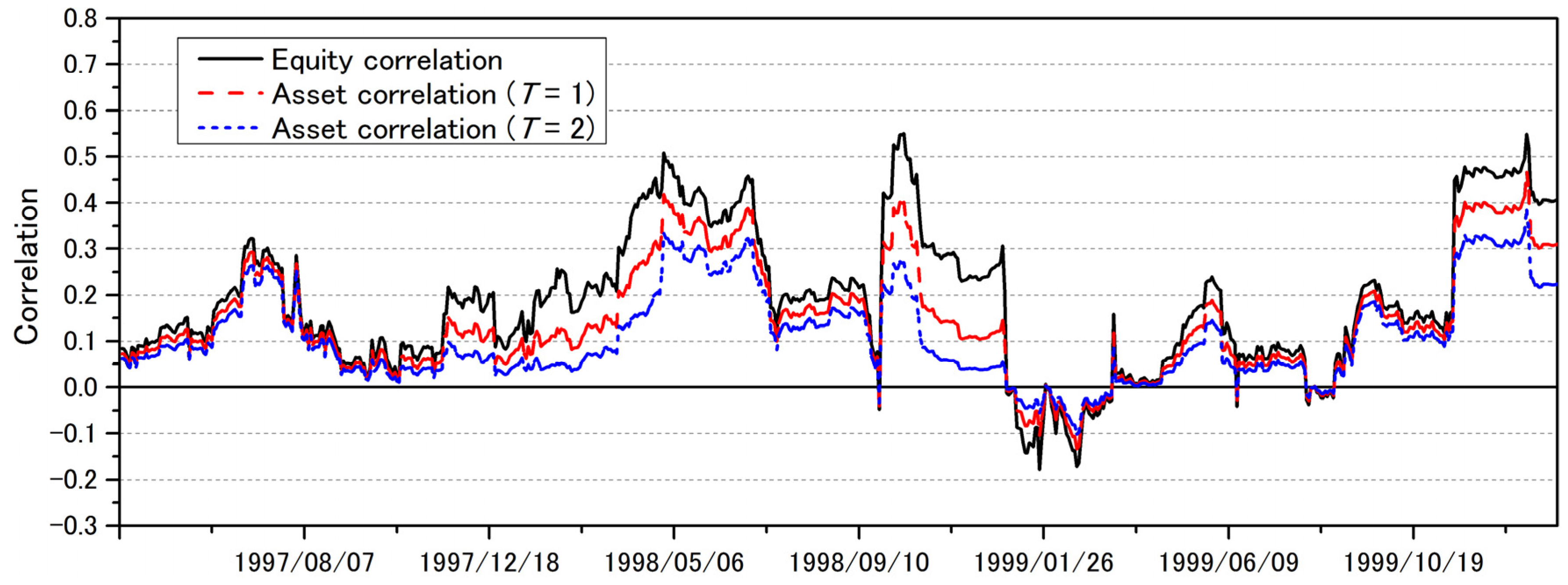
Figure 4, Figure 5 and Figure 6 show the change in the asset correlation calculated from (16) and the equity correlation. The asset correlation is calculated for evaluation periods of T = 1 year and T = 2 years. As shown in the figures, all asset correlations increase and decrease repeatedly within the range of the equity correlation, and the magnitude of the absolute values of asset correlation ${\rho }_{x(i,j)}$ and equity correlation ${\rho }_{s(i,j)}$ always obeys the relationship $\left|{\rho }_{x(i,j)}\right|\le \left|{\rho }_{s(i,j)}\right|$. As a result, the asset correlation is estimated based on the equity correlation, but the difference in value from the equity correlation depends on the size of the equity volatility and leverage at the time of estimation and the length of time. Thus, the equity volatility, leverage, and time are negatively related to asset correlation, and as they increase, the asset correlation becomes lower than the equity correlation.

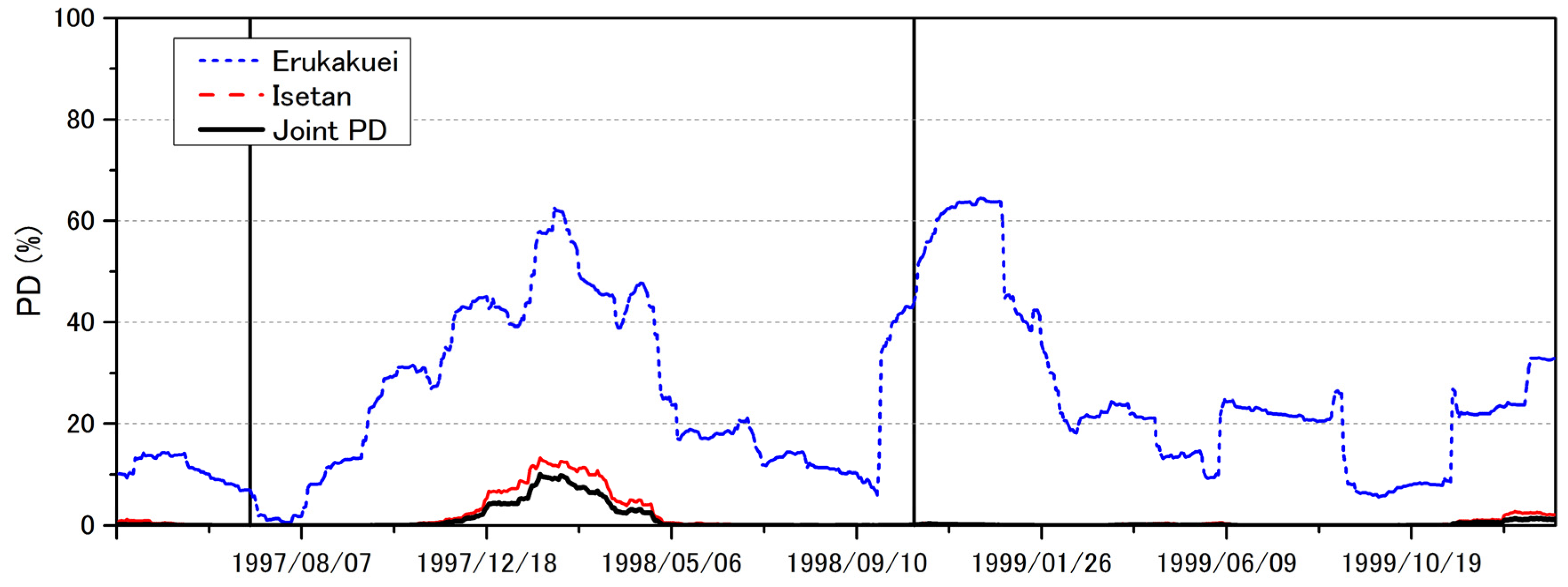
Figure 7, Figure 8 and Figure 9 show the changes in PD of the individual companies, as calculated from (15), and the joint PD between each pair of companies, as calculated from (17). The joint PD is consistently lower than the individual PD. Moreover, when the individual PD is high for both companies, so too is the joint PD. The Long-Term Credit Bank of Japan, which was the main financing bank for Erukakuei and Sogo, failed on 13 October 1998. Both companies were very closely related to this bank in terms of funding and personnel. Therefore, as shown in Figure 7, the joint PD increases after failure, and peaks at about 10%. However, Isetan is not influenced by this failure, and its PD remains low. Therefore, as shown in Figure 8 and Figure 9, the joint PD between Isetan and the other two companies is low. Conversely, the joint PD becomes high for all companies from July 1997 to the middle of 1998, as shown in Figure 7, Figure 8 and Figure 9. This coincides with the Asian Currency Crisis, which started when the Thai Baht collapsed after shifting from being pegged to the US Dollar to a floating exchange rate system on 2 July 1997. Thus, the joint PD changes with both the existence of a common risk factor in both companies and with the degree of influence of that factor.

Finally, the proposed method assumes that the volatility of equity and assets is constant regardless of the strike price and time, as in Merton’s model, and follows the Black–Scholes-type geometric Brownian motion. However, the implied volatilities calculated with actual market data are not constant, and the smile and skew phenomena have been observed. To solve this problem, recent academic and practical studies assume other stochastic processes. In a recent study, Yi et al. (2024) proposed an optimal portfolio strategy for two different risk assets by building a mixed model based on the constant elasticity of variance model and the jump-diffusion model.

7. Conclusions

Merton’s model for measuring credit risk has a clear conceptual basis, but it is not easy to apply to real data because of the difficulty of setting the model parameters. Various estimation methods for asset parameters have been proposed because of the difficulty of observing the asset values of a company. The calibration method, which uses observable stock prices to estimate the current asset value and volatility, is widely used. This paper has proposed a completely different approach that also uses stock prices for estimation, but estimates the asset parameters using Levy’s moment matching method. Our motivation for using the moment matching method was that it assumes random variables with similar characteristics, such as the average value and portfolio value of assets whose true distribution is unknown, follow a lognormal distribution.

The calibration method calculates two nonlinear equations, whereas the proposed method can estimate up to four different asset parameters from a single nonlinear equation if the current debt value is known. Thus, the proposed method enables simpler estimations than the calibration method in cases where a large number of asset parameters must be estimated. Empirical analysis showed that the proposed method gives similar asset parameters and PDs to the calibration method. The difference in the PDs given by the two methods was finally determined to be less than 2.2%. Hence, although the calculation procedure of the proposed method is very different from that of the calibration method, the asset parameters and PD can be estimated to the same degree of accuracy.

In the latter half of this paper, we focused on estimating the asset correlation between companies, allowing Merton’s model to be extended to multiple companies. Our results demonstrate that the proposed method can also estimate the asset correlation if the current debt value is known. As a result, the proposed method is extremely useful when the influence of equity volatility, leverage, and time must be considered in estimating the asset correlation based on the equity correlation. Further empirical analysis showed that the correlation obtained in this way changed less than that of equity under the influence of equity volatility, leverage, and time.

References

- Berg, Tobias. 2010. From actual to Risk-neutral Default Probabilities: Merton and Beyond. Journal of Credit Risk 6: 55–86. [Google Scholar] [CrossRef]
- Black, Fischer, and John C. Cox. 1976. Valuing Corporate Securities: Some Effects of Bond Indenture Provisions. Journal of Finance 31: 351–67. [Google Scholar] [CrossRef]
- Black, Fischer, and Myron Scholes. 1973. The Pricing of Options and Corporate Liabilities. Journal of Political Economy 81: 637–54. [Google Scholar] [CrossRef]
- Briys, Eric, and François de Varenne. 1997. Valuing Risky Fixed Rate Debt: An Extension. Journal of Financial and Quantitative Analysis 32: 239–48. [Google Scholar] [CrossRef]
- Cathcart, Lara, and Lina El-Jahel. 2004. Multiple Defaults and Merton’s Model. Working Paper. London: Tanaka Business School, Imperial College London. [Google Scholar]
- Collin-Dufresne, Pierre, and Robert S. Goldstein. 2001. Do Credit Spreads Reflect Stationary Leverage Ratios? Journal of Finance 56: 1929–58. [Google Scholar] [CrossRef]
- De Servigny, Arnaud, and Olivier Renault. 2002. Default Correlation: Empirical Evidence. Working Paper. New York: Standard & Poor’s. [Google Scholar]
- Duan, Jin-Chuan. 1994. Maximum Likelihood Estimation Using Price Data of the Derivative Contract. Mathematical Finance 4: 155–67. [Google Scholar] [CrossRef]
- Duffie, Darrell, and David Lando. 2001. Term Structures of Credit Spreads with Incomplete Accounting Information. Econometrica 69: 633–64. [Google Scholar] [CrossRef]
- Duffie, Darrell, and Kenneth J. Singleton. 2003. Credit Risk: Pricing, Measurement and Management. Princeton: Princeton University Press. [Google Scholar]
- Geske, Robert. 1977. The Valuation of Corporate Liabilities as Compound Options. Journal of Financial and Quantitative Analysis 12: 541–52. [Google Scholar] [CrossRef]
- Giesecke, Kay. 2003. Default and Information. Working Paper. Ithaca: Cornell University. [Google Scholar]
- Gupton, Gred M., Christopher Clemens Finger, and Mickey Bhatia. 1997. Credit Metrics-Technical Document. New York: JP Morgan. [Google Scholar]
- Hull, John C., and Alan D. White. 2001. Valuing Credit Default Swaps II: Modeling Default Correlations. Journal of Derivatives 8: 12–22. [Google Scholar] [CrossRef]
- Kealhofer, Stephen. 1993. Portfolio Management of Default Risk. Working Paper. San Francisco: KMV Corporation. [Google Scholar]
- Leland, Hayne E. 1994. Risky Debt, Bond Covenants and Optimal Capital Structure. Journal of Finance 49: 1213–52. [Google Scholar] [CrossRef]
- Leland, Hayne E., and Klaus Bjerre Toft. 1996. Optimal Capital Structure, Endogenous Bankruptcy and the Term Structure of Credit Spreads. Journal of Finance 50: 789–819. [Google Scholar]
- Levy, Edmond. 1992. Pricing European Average Rate Currency Options. Journal of International Money and Finance 11: 474–91. [Google Scholar] [CrossRef]
- Li, Weiping. 2016. Probability of default and default correlations. Journal of Risk and Financial Management 9: 7. [Google Scholar] [CrossRef]
- Longstaff, Francis A., and Eduardo S. Schwartz. 1995. A Simple Approach to Valuing Risky Fixed and Floating Rate Debt. Journal of Finance 50: 789–821. [Google Scholar] [CrossRef]
- Marcus, Alan J., and Israel Shaked. 1984. The Valuation of FDIC Deposit Insurance Using Option-Pricing Estimates. Journal of Money, Credit, and Banking 4: 446–60. [Google Scholar] [CrossRef]
- Merton, Robert C. 1973. Theory of Rational Option Pricing. Bell Journal of Economics and Management Science 4: 141–83. [Google Scholar] [CrossRef]
- Merton, Robert C. 1974. On the Pricing of Corporate Debt: The Risk Structure of Interest Rates. Journal of Finance 29: 449–70. [Google Scholar]
- Miyake, Masatoshi, and Hiroshi Inoue. 2009. A Default Probability Estimation Model: An Application to Japanese Companies. Journal of Uncer-tain Systems 3: 210–20. [Google Scholar]
- Øystein, Myhrer. 2012. Joint Default Probabilities: A Model with Time-Varying and Correlated Sharpe Ratios and Volatilities. Master’s thesis, Nor-ges teknisk-naturvitenskapelige universitet, Fakultet for samfunnsvitenskap og teknologiledelse, Institutt for sam-funnsøkonomi, Trondheim, Norway. [Google Scholar]
- Ronn, Ehud I., and Avinash K. Verma. 1989. Pricing Risk Adjusted Deposit Insurance: An Option-Based Model. Journal of Finance 41: 871–95. [Google Scholar]
- Scott, James. 1981. The Probability of Bankruptcy: A Comparison of Empirical Predictions and Theoretical Models. Journal of Banking and Finance 5: 317–44. [Google Scholar] [CrossRef]
- Vasicek, Oldrich A. 1984. Credit Valuation. Working Paper. San Francisco: KMV Corporation. [Google Scholar]
- Vassalou, Maria, and Yuhang Xing. 2004. Default Risk in Equity Returns. Journal of Finance 59: 831–68. [Google Scholar] [CrossRef]
- Yi, Haoran, Yuanchuang Shan, Huisheng Shu, and Xuekang Zhang. 2024. Optimal portfolio strategy of wealth process: A Lévy process model-based method. International Journal of Systems Science 6: 1089–103. [Google Scholar] [CrossRef]
- Zeng, Bin, and Jing Zhang. 2002. Measuring Credit Correlations: Equity Correlations are not Enough! Working Paper. San Francisco: KMV Corporation. [Google Scholar]
- Zhou, Chunsheng. 1997. A Jump-Diffusion Approach to Modeling Credit Risk and Valuing Defaultable Securities. Finance and Economics Discussion Series; Working Paper. Washington, DC: Board of Governors of the Federal Reserve System.
- Zhou, Chunsheng. 2001. An Analysis of Default Correlations and Multiple Defaults. Review of Financial Studies 14: 555–76. [Google Scholar] [CrossRef]
- Zhou, Chunsheng. 2011. The Term Structure of Credit Spreads with Jump Risk. Journal of Banking & Finance 25: 2015–40. [Google Scholar]
Figure 1.
Current asset value calculated using both methods.
Figure 2.
Asset volatility calculated using both methods.
Figure 3.
PD calculated using both methods.
Figure 4.
Erukakuei and Sogo (asset correlation calculated from (16) and equity correlation).
Figure 5.
Isetan and Sogo.
Figure 6.
Erukakuei and Isetan.
Figure 7.
Erukakuei and Sogo (PD of individual companies calculated from (15) and joint PD between two companies calculated from (17)).
Figure 8.
Figure 9.