Down-Side Risk Metrics as Portfolio Diversification Strategies across the Global Financial Crisis

Abstract

This paper features an analysis of the effectiveness of a range of portfolio diversification strategies, with a focus on down-side risk metrics, as a portfolio diversification strategy in a European market context. We apply these measures to a set of daily arithmetically-compounded returns, in U.S. dollar terms, on a set of ten market indices representing the major European markets for a nine-year period from the beginning of 2005 to the end of 2013. The sample period, which incorporates the periods of both the Global Financial Crisis (GFC) and the subsequent European Debt Crisis (EDC), is a challenging one for the application of portfolio investment strategies. The analysis is undertaken via the examination of multiple investment strategies and a variety of hold-out periods and backtests. We commence by using four two-year estimation periods and a subsequent one-year investment hold out period, to analyse a naive 1/N diversification strategy and to contrast its effectiveness with Markowitz mean variance analysis with positive weights. Markowitz optimisation is then compared to various down-side investment optimisation strategies. We begin by comparing Markowitz with CVaR, and then proceed to evaluate the relative effectiveness of Markowitz with various draw-down strategies, utilising a series of backtests. Our results suggest that none of the more sophisticated optimisation strategies appear to dominate naive diversification.

1. Introduction

It is now some sixty years since Markowitz [1] developed portfolio theory. Although it became a central foundation of classical finance, leading directly to the development of the capital asset pricing model (CAPM) by Sharpe [2], Lintner [3], Mossin [4] and Treynor [5], its practical application has been surrounded by difficulties. Markowitz [1,6] suggested choosing the portfolio with the lowest risk for a given level of portfolio return and defined such portfolios as being ‘efficient’. Merton [7] demonstrated the parabola that constitutes the efficient frontier in mean variance space.

Markowitz ([6] p. 206) states that: “Problems concerning the proper information to serve as the basic inputs concerning securities are outside the scope of this monograph. There are no magic formulas to supplant the sources of information and the rules of judgement of the security analyst”. The position of the efficient frontier has to be estimated and this leads to ‘estimation risk’. A common approach to portfolio selection is to use historical data to estimate the required means and covariances, but this leads to estimation risk, which, in turn, can lead to extreme and unstable portfolio weights over time. Michaud ([8] p. 3) suggests that: “The traditional MV [mean-variance] procedure often leads to financially irrelevant or false ‘optimal’ portfolios and asset allocations. In fact, equal weighting can be shown to be superior to MV optimization in some cases”. Michaud ([8] p. 33) also suggests that: ’MV optimizers are, in a fundamental sense, “estimation-error maximizers”. They have a tendency to over-weight (under-weight) those securities that have large (small) estimated returns, negative (positive) correlations and small (large) variances’. In turn, these are the securities likely to have the largest estimation errors.

One approach to adjusting for estimation risk involves the application of Bayesian techniques, and some of the original suggested adjustments were either based on the use of diffuse priors (see, for example, Barry [9] and Bawa et al. [10]) or ‘shrinkage’ estimators. The latter were explored by Jobson et al. [11], Jobson and Korkie [12] and Jorion [13,14]. More recent approaches have used an asset-pricing model to establish a prior; see, for example, Pástor (2000) and Pástor and Stambough [15,16].

Markowitz considered a number of downside risk measures as an alternative to mean-variance analysis [6,17], and similarly, as early as (1952), Roy developed his ‘safety-first’ asset selection criteria [18]. Rockafellar et al. [19,20,21] developed the mean-deviation approach to portfolios as an extension to the classic mean-variance approach generalising the results to the one fund theorem, [19], the CAPM [20], plus the derivation of market equilibrium for investors using different deviation measures [21]. More recently, Zabarankin et al. [22] have extended the CAPM with a draw-down measure to measure betas and alphas based on draw-downs.

We draw on several of these portfolio optimisation approaches in the empirical work in this paper, namely: naive diversification, Markowitz mean variance analysis with positive constraints, conditional value at risk (CVaR), conditional draw-down (CDaR), average draw-down (AveDD), maximum-draw-down (MaxDD), plus draw-down metrics set at 95% confidence levels (CDaR95) and (CDaRmin95). We test their out-of-sample capabilities in times of market turbulence in a series of hold-out and backtests.

The paper is organised into five sections; this Introduction is followed by a discussion of research methods in Section 2, which discusses the various portfolio optimisation strategies adopted beginning with naive diversification and then proceeding to Markowitz mean-variance analysis, CVaR and a variety of optimal draw-down approaches. Section 3 introduces the dataset and its characteristics, while Section 4 presents the results, and a brief conclusion follows in Section 5.

2. Research Method

We proceed by adopting a variety of portfolio selection approaches and adopt a naive portfolio benchmark with 1/N weights as a comparator. This approach was also used by DeMiguel et al. [23], in an out-of-sample analysis, of the mean-variance portfolio selection criteria, employing U.S. data sets, plus a variety of adjustments for estimation risk. They concluded that there are still “many miles to go” before the gains promised by portfolio optimisation techniques can be realised out of sample.

Our focus is broader than theirs, in that we employ a variety of portfolio optimisation techniques that go well beyond mean-variance optimisation. We contrast naive diversification, with mean-variance analysis, plus other portfolio optimisation techniques, such as the optimisation of conditional value at risk (CVaR), and other techniques, such as various draw-down strategies, and our analysis is conducted across the major European equity markets.

2.1. Naive 1/N Diversification Strategy

In this strategy, we just consider holding a portfolio where the weights for the asset ${\omega }_j=1/N$, which is applied for each of the N risky assets. This strategy ignores the data and does not involve any estimation or optimisation. DeMiguel et al. [12] suggest that this can be considered as equivalent to imposing the restriction that ${\mu }_t\propto {\sum }_t{1}_N$ for all t, implying that expected returns are proportional to total risk rather than systematic risk.

2.2. Markowitz Mean-Variance Analysis

Markowitz [1] founded modern mathematical finance and ushered in formal portfolio analysis in one giant step with his introduction of the mean-variance model of the risk-return relationship. Variance is an appropriate risk-measure if either the investor’s utility set is quadratic or the return series considered are multivariate normal.

The Markowitz [1] approach can be presented as the following non-linear-programming problem.

$$\begin{array}{c}min\\ \omega \end{array}{\displaystyle \frac{1}{n}}{\displaystyle \sum _{i=1}^n}{\left({\displaystyle \sum _{j=1}^m}{\omega }_j(r_{i,j}-{\mu }_j)\right)}^2$$

$$s.t.$$

$${\displaystyle \sum _{j=1}^m}{\omega }_j{\mu }_j=C$$

(1)

$${\displaystyle \sum _{j=1}^m}{\omega }_j=1$$

$${\omega }_j⩾0,\forall j\in \left\{1,....,m\right\}.$$

In the above formulation, ω are the portfolio weights for the universe of the $j=1,....m$ assets available, $i=1,....,n$ are the number of periods considered for the returns r and for ${\mu }_j$, which is the forecast return. The optimisation involves minimizing the portfolio variance subject to the portfolio forecast return being set to a level C. A full investment constraint and positive constraints on the weights are included, effectively ruling out short sales. In our subsequent analyses, we apply mean-variance optimisation with both a positive weight constraint and with an upper limit on the weight of any one security being less than 0.4% or 40% of the chosen portfolio.

Jagganathan and Ma [24] demonstrate that the placement of a short-sale constraint on the minimum variance portfolio is equivalent to shrinking the elements of the covariance matrix. For this reason, we do not make any other adjustments for estimation risk. See, for example, the discussions in Best and Grauer [25], Chan, Karceski and Lakonishok [26] and Ledoit and Wolf [27].

2.3. Optimising Conditional Value at Risk

Uryasev and Rockafellar [28] in a series of papers have advocated CVaR as a useful risk metric. Pflug [29] proved that CVaR is a coherent risk measure with a number of attractive properties, such as convexity and monotonicity, among other desirable characteristics. A number of papers apply CVaR to portfolio optimization problems; see, for example, Rockafeller and Uryasev [30], Andersson et al. [31], Alexander, Coleman and Li [32], Alexander and Baptista [33] and Rockafellar et al. [19].

The conditional value at risk of X at level $\alpha \in (0,1)$ is defined by:

$$CVa{R}_{\alpha }\left(X\right)=expectationofXinits\alpha -tail,$$

(2)

which can also be expressed as:

$$CVa{R}_{\alpha }\left(X\right)={\displaystyle \frac{1}{1-\alpha }}{\int }_{\alpha }^{1}Va{R}_{\tau }\left(X\right)dt.$$

(3)

Pffaf ([34] p. 223) recapitulates Uryasev [35], noting that the following risk measures are needed in order to define CVaR:

• $Va{R}_{\alpha }$, the α quantile of a loss distribution;
• $CVa{R}^{+}$, the expected losses strictly exceeding VaR (i.e., mean excess loss or expected shortfall);
• $CVa{R}^{-}$, the expected losses that are weakly exceeding VaR, i.e., losses that are equal to or exceed VaR.

The CVaR is then defined as a weighted average between VaR and $CVa{R}^{+}$:

$$CVaR=\lambda VaR+(1-\lambda )CVa{R}^{+},$$

(4)

where the weight $0\le \lambda \le 1$ is given by $\lambda =\left(\psi \right(VaR)-\alpha )/(1-\alpha )$ and $\psi \left(VaR\right)$ denotes the probability that losses do not exceed or are equal to VaR for a given confidence level.

Rockafellar and Uryasev ([36] p. 22) further elaborate on some of these issues in their discussion of the ‘fundamental risk quadrangle’, and suggest a way round the issue of the non-elicitability of CVaR by utilising quantile regression, as pioneered by Koenker and Basset [37]. Fissler and Ziegel [38] further concur, in a discussion of higher order elicitability and Osbond’s principle, and again mention quantile and expectile regression. They demonstrate that the pair (value at risk, expected shortfall) is elicitable, subject to mild regularity assumptions, which involve the relevant distributions consisting of absolutely continuous distributions with unique quantiles. This does not seem unreasonable in the case of financial return distributions.

In terms of portfolio selection, CVaR can be represented as a non-linear programming minimisation problem with an objective function given as:

$$\begin{array}{c}min\\ \omega ,\upsilon \end{array}{\displaystyle \frac{1}{na}}{\displaystyle \sum _{i=1}^n}\left[max(0,\upsilon -{\displaystyle \sum _{j=1}^m}{\omega }_j{r}_{i,j})\right]-\upsilon$$

(5)

where υ is the α-quantile of the distribution. In the discrete case, this was shown by Rockefellar and Uryasev [28] to be capable of being represented by using auxiliary variables in the linear programming formulation below:

$$\begin{array}{c}min\\ \omega ,d,\upsilon \end{array}{\displaystyle \frac{1}{na}}{\displaystyle \sum _{i=1}^n}{d}_i+\upsilon$$

$$s.t.$$

$${\displaystyle \sum _{j=1}^m}{\omega }_j{r}_{i,j}+\upsilon \ge -d_i,\forall \in \left\{1,\dots ,n\right\}$$

$${\displaystyle \sum _{j=1}^m}{\omega }_j{\mu }_j=C$$

(6)

$${\displaystyle \sum _{j=1}^m}{\omega }_j=1$$

$${\omega }_j\ge 0,\forall j\in \left\{1,....,n\right\}$$

$$d_i\ge 0,\forall i\in \left\{1,....,n\right\}$$

where υ represents the VaR at the α coverage rate and $d_i$ the deviations below the VaR.

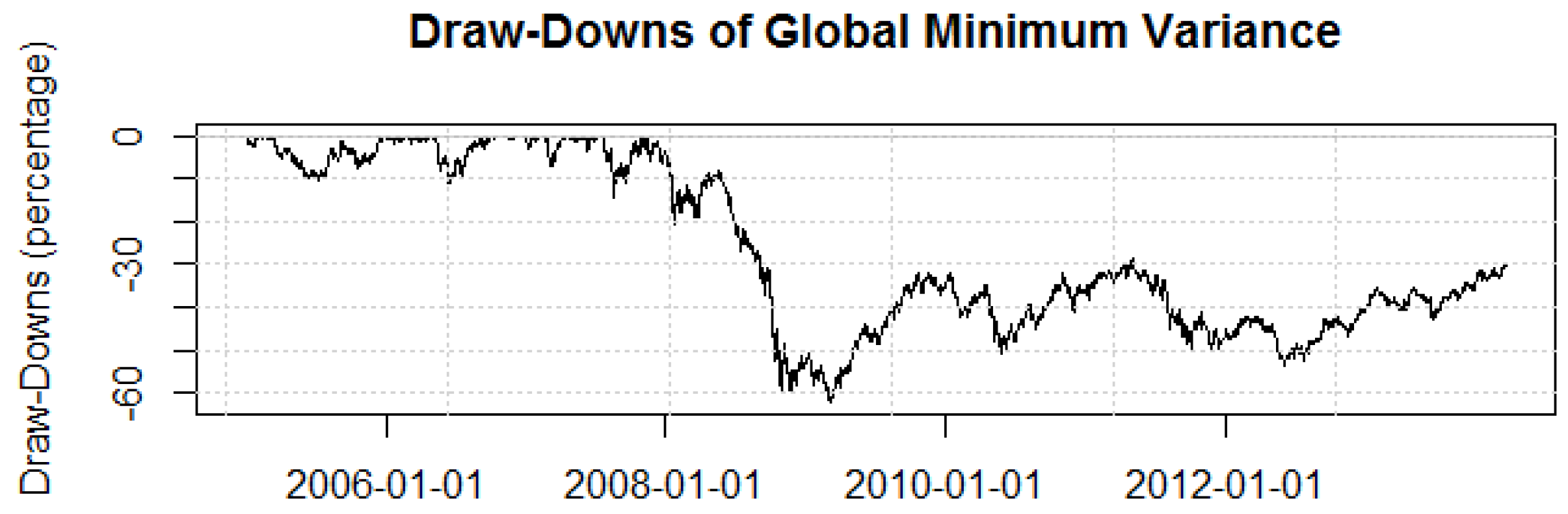
2.4. Optimal Draw-Down Portfolios

Chekhlov et al. [39,40,41] considered the optimization of portfolios with respect to the portfolio’s draw-down. The conditional draw-down (CDD) measure includes the maximum draw-down (MaxDD) and average draw-down (AvDD) as its limiting cases. The CDD family of risk functional measures is similar to CVaR. Chekhlov et al. [41] suggest that portfolio managers would like to avoid large draw-downs and/or extended draw-downs, as this may lead to a loss of mandate or withdrawal of business.

The analysis can be developed as follows; let a portfolio be optimised over some time interval $[0,T]$, and let $W\left(t\right)$ be the portfolio value at some moment in time $t\in [0,T]$. The portfolio draw-down is defined as:

$$ma{x}_{\tau \in [0,t]}W\left(\tau \right)-W\left(t\right)/W\left(t\right)$$

(7)

If we think in terms of the portfolio’s constituent assets and write $W(\omega ,t)=y_t^{\prime }\omega$ as the un-compounded portfolio value at time t, with ω the portfolio weights for the N constituent assets and write $y_t$ for the cumulated returns, the draw-down can be written as:

$$D(\omega ,t)=\underset{0\le \tau \le t}{max}\left\{W(\omega ,\tau )\right\}-W(\omega ,t)$$

(8)

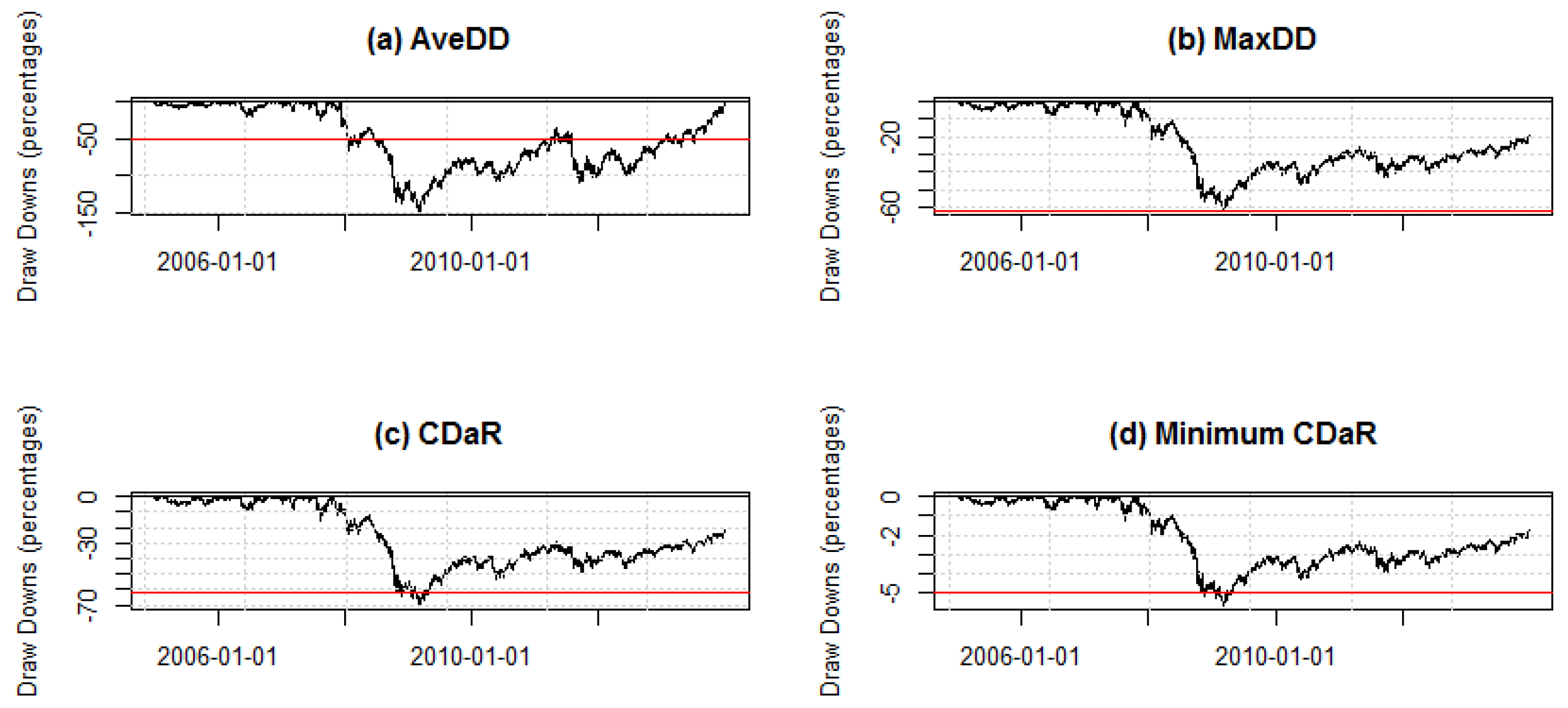
This definition can be converted into the three previously-mentioned functional risk measures; MaxDD, AvDD and conditional draw-down at risk (CDaR). CDaR is dependent on the chosen confidence level α in the same way that CVaR is. CDaR can be defined as:

$$CDaR{\left(\omega \right)}_{\alpha }=\underset{\varsigma }{min}\{\varsigma +{\displaystyle \frac{1}{(1-\alpha )T}}{\int }_0^T{[D(\omega ,t)-\varsigma ]}^{+}dt$$

(9)

where ς is the threshold value for draw-downs so that only $(1-\alpha )T$ observations exceed this value. The limiting cases of this family of risk functions are MaxDD and the AvDD. In the case that $\alpha \to 1$, CDaR approaches the maximum draw-down, $CDaR{\left(\omega \right)}_{\alpha \to 1}=MaxDD\left(\omega \right)=ma{x}_{0\le t\le T}\{D(\omega ,t)dt$. The AvDD results from the case in which $\alpha =0$. That is, $CDaR{\left(\omega \right)}_{\alpha \to 0}=AvDD\left(\omega \right)=(1/T{\int }_0^{T}D(\omega ,t)dt$.

These risk functionals can be used in terms of the optimization of a portfolio’s draw-down and implemented as inequality constraints for a fixed share of the wealth at risk.

The goal of maximizing the average annualised portfolio return with respect to limiting the maximum draw-down can be written:

$$P_{MaxxDD}=\underset{\omega ,u}{arg}maxR\left(\omega \right)={\displaystyle \frac{1}{dC}}{y}_T^{\prime }\omega ,$$

(10)

$$u_k-y_k^{\prime }\omega \le v_{1}C,$$

$$u_k\ge y_k^{\prime }\omega ,$$

$$u_k\ge u_{k-1},$$

$$u_0=0,$$

where u denotes a $(T+1\times 1)$ vector of slack variables in the program formulation, in effect the maximum portfolio values up to time period k with $1\le k\le T$.

We include these three approaches to portfolio optimisation, CDaR, MaxDD and AvDD, in our portfolio analyses. We use programs from the R library to conduct our analyses, in particular, the packages fPortfolio, FRAPO and PerformanceAnalytics. We also modify R code from Pfaff [34] to undertake the various draw-down optimisations.

The above approaches to portfolio analysis can be characterised under the general heading of operational research methods featuring applications of multi-criteria optimization methods to portfolio selection problems. Surveys of various aspects of this literature are provided by Sawik [42,43,44].

The application of coherent risk measures has generated a large literature, which attempts to extend their application to a dynamic context in a variety of different ways. For applications of these approaches see the early work by Riedel [45] or the more recent survey by Acciaio and Penner [46]. This area of the literature is still being developed and is based on the previously-mentioned coherent risk measures of Artzner et al. [47]. Their original approach, based on the capital requirements framework, is the framework adopted in our paper. Delbaen [48] and Follmer and Schied [49] provide a comprehensive presentation of the theory of static coherent and convex risk measures. The most recent comprehensive application of this approach to portfolio selection is provided by Rujeerapaiboon et al. [50].

Platen and Heath [51] embark on an initially different approach in a probabilistic Markovian framework in their benchmark approach to quantitative finance. A central component of these approaches is the use of the ‘growth optimal portfolio’ (GOP). The GOP is the portfolio that has the maximal expected growth rate over any time horizon. This strictly positive portfolio almost surely outperforms any other strictly positive portfolio over a sufficiently long time horizon, as first noted by Kelly [52].

Although Kelly’s strategy promise of doing better than any other strategy seems compelling, some economists have argued strenuously against it, mainly because an individual’s specific investing constraints override the desire for optimal growth rate. The conventional alternative is utility theory, which says bets should be sized to maximize the expected utility of the outcome (to an individual with logarithmic utility, the Kelly bet maximizes utility, so there is no conflict in this case). The Kelly approach assumes the only important thing is long-term wealth. Most people also care about the path to get there. Kelly betting leads to highly volatile short-term outcomes, which many people find unpleasant, even if they believe they will do well in the end. Samuelson [53,54], in particular, was a long time critique of the Kelly criterion.

3. Dataset

We utilise a sample of the daily values of ten European Stock Indices taken from Datastream for a period from the beginning of 2005 to the end of 2013, all constituted in U.S. dollar terms. The nine-year sample period, which incorporates the period of both the Global Financial Crisis (GFC) and subsequent European Debt Crisis (EDC), is a challenging one for the application of portfolio investment strategies. The ten markets and indices involved are: the FTSE100 index, the DAX index, the CAC 40 index, the AEX Amsterdam Index, the IBEX 35 Index the OMX Copenhagen 20 Index, the OMX Stockholm All Share Index, the OMX Helsinki All Share Index, the BVLG PSI Portuguese General Index and the BFX Belgian 20 Index. The end of day values of these indices are differenced in to form arithmetically-compounded return series. Graphs of the returns on these indices, for the whole sample period, are shown in Figure 1 and QQ plots in Figure 2.

It is clear from the QQ plots, in Figure 2, that all of the index return distributions are non-normal and fat-tailed. This has implications for the use of Markowitz’s method to select efficient portfolios, given that it is based on the assumption of multivariate normal distributions. These issues are discussed by Rachev and Mittnik [55], Ortobelli et al. [56], Rachev et al. [57,58].

If it is assumed that the fat-tailed distributions observed conform to stable Paretian distributions, then several attractive properties follow as observed by Rachev et al. [57]. The appeal of the stable non-Gaussian approach is given by its attractive properties that are almost the same as the normal one. A relevant desirable property of the stable distributional assumption is that stable distributions have the domain of attraction. The central limit theorem for normalized sums of i.i.d. random variables determines the domain of attraction of each stable law. Therefore, any distribution in the domain of attraction of a specified stable distribution will have properties close to those of the stable distribution. They discuss the potential attractiveness of a three-fund separation model for asset pricing and risk assessment. Rachev et al. [58] summarise their current practical applied position on these issues and suggest that expected tail loss (ETL) or conditional value at risk (CVaR) is a suitable portfolio risk metric under these conditions. This is one of the approaches to portfolio optimisation adopted in the current study. We do not deviate from the standard Markowitz approach, in our empirical analysis, because it is so commonly applied in practice, and it is informative to see how it compares.

Descriptive statistics for the series are given in

Table 1. Descriptive statistics of indices’ daily arithmetically-compounded returns.

	Mean	Median	Min	Max	SD	Skewness	Ex. Kurtosis	Hurst Exponent
AEX	0.000209306	0.000604318	−0.111806	0.131065	0.0168772	0.151445	8.60375	0.552931
BFX	0.000135558	0.000391543	−0.0906908	0.110042	0.0161834	0.0177818	5.29293	0.570771
BVL	0.0000685788	0.000296413	−0.121168	0.111047	0.0152447	0.0657292	7.74367	0.586224
DAX	0.000497582	0.000730373	−0.0915454	0.131672	0.0171735	0.177855	6.46489	0.535675
FCH	0.000215969	0.000403166	−0.110744	0.129115	0.0179219	0.271767	6.96039	0.521829
FTSE	0.0002	0.0006	−0.10002	0.129967	0.0153948	0.150327	9.69932	0.533963
IBEX	0.000218544	0.000198572	−0.101087	0.161465	0.0187440	0.302523	6.79814	0.558791
OMXC	0.000463244	0.000820621	−0.130423	0.118779	0.0163018	−0.0765109	6.65507	0.576929
OMXH	0.000228989	0.000135171	−0.0968762	0.104224	0.0175208	0.126917	4.20111	0.576929
OMXSP	0.000462738	0.000652458	−0.0960500	0.133513	0.0192538	0.203474	4.99464	0.541169

.

The descriptive statistics in Table 1 suggest that the series have the typical characteristics on financial return series in that they are skewed, mainly positively, but the OMXC series demonstrates negative skewness. They all demonstrate excess kurtosis and some evidence of long memory, in that the Hurst coefficient for all of them is above 0.5. This suggests that portfolio analysis based on mean variance analysis is not likely to match the characteristics of the data, as was discussed earlier in this section.

The choice of indices was determined by availability in the Thomson Reuters Datastream subscription in force at Edith Cowan University at the time of data downloading. A number of caveats should be made about the construction of the indices. All are capitalization-weighted indices, but some of the indices, such as the CAC 40, represent the more liquid, highly capitalized companies in the market and should be more readily replicable in an investment strategy. Other indices, such as the OMX Helsinki all share, represent the total market, would include less liquid companies and therefore be less easy to replicate. Most of the indices, with the exception of the BVLG Portuguese Index and the DAX, are not total return indices and, therefore, do not include adjustments for re-invested dividends. The total return indices are likely to have higher returns. This is partially supported by the descriptive statistics in Table 1. The Dax has the highest mean return at 0.000497, yet the second highest mean return is that of the OMX Copenhagen 20 with a value of 0.00046. The position is reversed in terms of the median return, with OMXC recording 0.00082 and the DAX 0.00073, yet the total return version of the OMX 20 was not available to us.

4. Results

4.1. Naive Diversification versus Markowitz Portfolios

The analysis commenced with a naive set of portfolios calculated for an annual holding period for each year with portfolio weights of 1/N. The results are shown in the second to fifth columns of

Table 2. Portfolio optimisation results’ yearly hold-out samples.

	Naive Diversification				Markowitz Pos.Constraints (Max Weight 0.4)
	Indices Included	Equal Weights ${\displaystyle \frac{1}{N}}$ Return			Indices Included (Weights)
		Return (%)	SD	Sharpe Ratio		Return (%)	SD	Sharpe Ratio
2007	All	0.00058263	0.010669	0.0546	Dax(0.4) OMXC(0.4) OMXSP(0.2)	0.00069980	0.011182	0.0625
2008	All	−0.0027037	0.026519	−0.1019	Dax(0.4) OMXC(0.4) OMXSP(0.2)	−0.00248078	0.0269006	−0.0922
2009	All	0.0011225	0.019535	0.05746	Dax(0.4) OMXC(0.4) OMXSP(0.2)	0.0011954	0.020944	0.04927
2010	All	0.000076592	0.016380	0.00467	Dax(0.4) OMXC(0.4) OMXSP(0.2)	0.00070664	0.00054330	1.3006
2011	All	−0.00072393	0.019653	−0.0368	Dax(0.4) OMXC(0.4) OMXSP(0.2)	−0.00061439	0.020027	−0.03067
2012	All	0.0051752	0.013875	0.3729	Dax(0.4) OMXC(0.4) OMXSP(0.2	0.00092886	0.013461	0.06900
2013	All	0.00083955	0.0096324	0.0871	Dax(0.4) OMXC(0.4) OMXSP(0.2	0.00097143	0.0098360	0.09876

. Portfolios were also calculated using Markowitz mean/variance analysis with all of the portfolio weights constrained to be positive, and an upper limit of 0.4 was set on the holding of any individual security. The analysis was conducted over a two-year sample period; the optimal portfolio weights were calculated, and then, these were applied to a portfolio held for a subsequent period of one year. The analysis suggested that the optimal portfolio throughout the sample period consisted of 0.4 invested in the DAX, 0.4 invested in the OMXC and 0.2 invested in the OMXSP. The focus on these three individual markets is not surprising given that Table 1 reveals that these markets have the highest returns over the sample period.

The outcomes for the one-year holding periods are shown in Columns 6–9 in Table 2. The naive diversification strategy gives a higher return in one year; 2012. However, when risk is also taken into account, the naive portfolio has higher Sharpe ratios in 2009 and in 2012, and so, on balance, the results favour the Markowitz with constraints in five of the seven years considered.

The results in

Table 3. Markowitz with positive constraints, 1-year hold-out results.

Markowitz Pos. Constraints
Year	Indices Included (Weights)	Return (%)	SD	Sharpe Ratio
2007	FTSE(0.32) + OMXC(0.014) + BVLG(0.66)	0.00058082	0.0091520	0.063
2008	AEX(0.17) + IBEX(0.05) + BVLG(0.78)	−0.00256311	0.0251282	−0.102
2009	GDAX(0.12) + BVLG(0.69) + BFX(0.19)	0.00127888	0.016421	0.077
2010	BVLGRET(0.86) + BFXRET(0.14)	−0.000526745	0.0175202	−0.0.0301
2011	FTSE(0.36) + OMXC(0.15) + BVLG(0.49)	−0.000539713	0.0149820	−0.0360
2012	FTSE(0.77) + OMXC(0.22) + BVLG(0.01)	0.000565371	0.0109104	0.0518
2013	FTSE(0.66) + OMXC(0.26) + BVLG(0.08)	0.000648125	0.00798428	0.0812

suggest that the Markowitz optimisation with positive weights produces a higher Sharpe ratio in the one-year hold out sample in 2007, 2009 and 2010 only and in the other four periods has an inferior outcome. This is consistent with the previous findings of DeMiguel et al. [23], who suggested that in their sample and simulation analysis, it took around 3000 months with a portfolio of 25 assets to outperform the naive diversification strategy.

4.2. Markowitz versus CVaR Portfolios

In the next part of the analysis, we compared a standard Markowitz optimisation with an optimisation procedure based on the risk measure CVaR. We set the confidence level to two alternatives, 10% and 20%; the confidence level is specified in return and not in loss space, hence a value of 0.1 coincides with the 90% level of the loss distribution. The backtest is constructed with respect to prior data history of 250 daily observations or approximately the previous year. The portfolios are optimised with respect to this sliding data window, and the results are determined by the sample values in this sliding data window. We use this one-year period to estimate the weights for both the Markowitz and CVaR portfolios and then roll the window forwards through the datasets to conduct our backtests. We use two different quantiles to set the CVaR parameters at 10% and 20%, respectively. We employ the R (3.30) packages FRAPO and fPortolio and modify some of the R code provided in Pfaff [34]. Plots of the results are shown in Figure 3.

It is clear in Figure 3 that if the quantile for the CVaR is set to 0.1, for the purposes of the backtest, that there are very few occasions when CVaR outperforms minimum variance with positive constraints, when applied to this European set of markets, over the recent nine-year sample period. The plot for CVaR (blue line) in the first diagram in Figure 3 is predominantly below the plot of the Markowitz outcome (black line). This is clear in the second diagram in which the plot for the difference between the CVaR and minimum variance outcomes in blue very rarely pierces the horizontal line at zero, at the top of the diagram, and ventures into positive territory.

The outcomes change to a considerable degree when we alter the quantile for the CVaR optimisation to 0.2. The results of this second analysis are shown in Figure 4. There is no longer uniform dominance by the minimum variance portfolio, and for for a prolonged period in 2010–2011, the CVaR portfolio has superior outcomes; but, over the entire backtest, it is still inferior. This is indicated by the summary statistics for the two separate backtests of the CVaR versus minimum variance strategy in

Table 4. Backtests’ minimum CVaR versus minimum variance.

	CVaR(0.1) - Min Var	CVaR(0.2) - Min Var
Min	−9.294	−2.7527
1st Qu.	−7.678	−1.1399
Median	−5.544	−0.5865
Mean	−5.112	−0.3207
3rd Qu.	−2.324	0.3218
Max	0.604	3.6258

.

It can be seen in Table 4 that CVAR used as an optimiser at both the 0.1 and 0.2 quantiles is still inferior, in that the mean and median differences are still negative. The CVaR(0.2) works better, but the mean and median differences are still negative. There is the further problem that ex ante, it is difficult to know what is the appropriate quantile to pick for the CVaR optimisation.

Table 5. Average portfolio weights GMVand Min CVaR through rolling windows.

	FTSE	GDAX	FCH	AEX	IBEX	OMXC	OMXS	OMXH	BVL	BFX
GMV Weights	0.380222	0.044829	0	0.006797	0.00049	0	0.111106	0 0.003272	0.424209	0.029075
Weights CVaR (0.1)	0.344506	0.047293	0	0.000478	0.002555	0.132861	0.003192	0.010384	0.443938	0.014793
Weights CVaR (0.2)	0.33971665	0.064228	0.0	0 0.002498	0.00689	0.142548	1.09E-10	0.007579	0.435044	0.001496

shows the average weights applied in the rolling windows in the optimisation techniques. On average, the Markowitz minimum variance portfolios place greater weight on the FTSE, average weight 0.38, OMXS with an average of 0.11 and BVL with an average weight of 0.424. The CVaR techniques still emphasize the FTSE, but with an average weight of 0.04 less than GMV, put slightly more emphasis on the DAX, much greater emphasis on OMXC at around 0.13–0.14, given that it was not included in the GMV. They drop investment in OMXS and increase the weight in BVL.

However, they both perform worse than Markowitz optimisation, which in the previous analysis was shown to be inferior to naive diversification for this sample set of European markets for this particular nine-year period, which includes the GFC and the European debt crisis.

4.3. Draw-Down Portfolio Analyses

Figure 5 shows the draw-downs of the global minimum variance portfolio.

The trajectory of draw-downs of the global minimum variance portfolio, as shown in Figure 5, reflects the initial shock of the GFC, on European markets, followed by the continuing impact of the European Sovereign debt crisis. The period from 2007 onwards has been a tough time for investors in European markets.

A comparison of the draw-downs for the various strategies is shown in Figure 6. The analysis program is coded to use the global minimum variance portfolio as a benchmark allocation for long-only investments. The characteristics of this solution are compared to the allocations of portfolios that are restricted by their maximum, average and conditional draw-downs and with a minimum conditional draw-down at risk portfolio. The imposition of an average draw-down constraint to optimise the portfolio can still result in large draw-downs, as shown in the first graph labelled “(a) AveDD” in the top left-hand panel of Figure 6. The draw-down of −150% is much greater than the other draw-down optimiser outcomes, with the minimum CDaR, in panel (d) of Figure 6, producing the smallest draw-down, relative to global minimum variance portfolio benchmark.

In

Table 6. Comparison of portfolio allocations and characteristics. MaxDD, maximum draw-down; AveDD, average draw-down; CDaR, conditional draw-down.

	GMV	MaxDD	AveDD	CDaR95	CDaRMin95
FTSE
Weight	0.393953078	1.00	0.00	1.00	1.00
MES	0.029383168	0.019985	0.00	0.022582148	0.001812922
MPR	0.393953078	1.00	0.00	1.00	1.00
GDAXI
Weight	0.00	0.00	1.00	0.00	0.00
MES	0.00	0.00	0.034926	0.00	0.00
MPR	0.00	0.00	1.00	0.00	0.00
FCHI
Weight	0.00	0.00	0.00	0.00	0.00
MES	0.00	0.00	0.00	0.00	0.00
MPR	0.00	0.00	0.00	0.00	0.00
AEX
Weight	0.00	0.00	0.00	0.00	0.00
MES	0.00	0.00	0.00	0.00	0.00
MPR	0.00	0.00	0.00	0.00	0.00
IBEX
Weight	0.00	0.00	0.00	0.00	0.00
MES	0.00	0.00	0.00	0.00	0.00
MPR	0.00	0.00	0.00	0.00	0.00
OMXC20
Weight	14.37856	0.00	0.00	0.00	0.00
MES	0.029383168	0.00	0.00	0.00	0.00
MPR	14.37856	0.00	0.00	0.00	0.00
OMXSPI
Weight	0.00	0.00	0.00	0.00	0.00
MES	0.00	0.00	0.00	0.00	0.00
MPR	0.00	0.00	0.00	0.00	0.00
OMXHPI
Weight	0.00	0.00	0.00	0.00	0.00
MES	0.00	0.00	0.00	0.00	0.00
MPR	0.00	0.00	0.00	0.00	0.00
BVLG
Weight	46.22613	0.00	0.00	0.00	0.00
MES	0.029383168	0.00	0.00	0.00	0.00
MPR	46.22613	0.00	0.00	0.00	0.00
BFX
Weight	0.00	0.00	0.00	0.00	0.00
MES	0.00	0.00	0.00	0.00	0.00
MPR	0.00	0.00	0.00	0.00	0.00
Overall
ES95%	2.9383168	1.9985201	3.4926388	2.2582148	0.1812922
DivRatio	1.078599	1.000	1.000	1.000	1.000

, we further analyse these portfolios fitted to historic data in terms of their weights, risk contributions and diversification ratios.

In Table 6, we show how the portfolio weights vary if we apply the various strategies across the entire nine-year sample period. The GMV strategy with positive weights places 39% of the portfolio in the FTSE, nearly 15% in OMXC20 and the remainder of around 46% in BVLG. The other strategies, which concentrate on minimising the maximum draw-down, average draw-down, or conditional average draw-downs, or minimum draw-downs at a 95% confidence level produce much less diversified portfolios, with MaxDD placing 100% in the FTSE, AveDD placing 100% in the DAX and CDaR95 and CDaRMIN95, both placing 100% in the FTSE.

The impact on reducing diversification is shown in the bottom line of Table 6, which reports the diversification ratio, which is lower for all of the CDaR-based strategies than the minimum variance one, which is the entry at the bottom of the first column. The diversification ratio was developed by Choueifaty and Cognard [59] and Choueifaty et al. [60] and provides a measure of the degree of diversification of long-only portfolios. It has a lower bound of one, which is achieved in single asset portfolios.

Paradoxically, optimising by reducing the average draw-down produces a higher expected shortfall at the 95% level than the mean variance optimiser, as shown in the penultimate entry in the fourth column of Table 6, and this is consistent with the graphical analysis presented in Figure 6.

These results are obtained by fitting the optimisations to the entire dataset and are of limited use. The crucial tests are the out of sample ones, and these are considered next, using rolling one-year windows for estimation purposes. In the next section of the analysis, we compute the draw-down portfolio solutions and use the maximum draw-down of the minimum variance portfolio as a benchmark value. The CDaR portfolios are calculated for a confidence level of 95%.

4.4. Portfolio Comparisons Using Backtests

We conducted further analyses to compare the results of the minimum variance strategy with the various conditional draw-down at risk strategies. The backtests are carried out using a recursive window of 250 days, or one year of daily data. The CDaR portfolio is optimised for a conditional draw-down of 10% at a 95% confidence level. The GMV portfolio is again constrained to be long only.

Figure 7 provides a graph of the wealth trajectories of the CDaR strategy contrasted with the GMV one. An initial wealth of 100 units is assumed. There are two periods in 2013 when the wealth trajectory of the GMV portfolio falls well below that of the CDaR strategy, which is much less volatile, but by the end of the period, the GMV trajectory is well above that of the CDaR portfolio.

Table 7. Drawdowns comparison.

	Draw-downs(MVRet)
	From	Trough	To	Depth	Length	To Trough	Recovery
1	4/02/2013	24/06/2013	19/09/2013	−0.1216	164	101	63
2	23/10/2013	1/11/2013	28/11/2013	−0.0299	27	8	19
3	2/12/2013	13/12/2013	23/12/2013	−0.0289	16	10	6
4	20/09/2013	9/10/2013	14/10/2013	−0.0279	17	14	3
5	16/01/2013	16/01/2013	17/01/2013	−0.0081	2	1	1
	Draw-downs(CDRet)
	From	Trough	To	Depth	Length	To Trough	Recovery
1	4/02/2013	24/06/2013	16/09/2013	−0.013	161	101	60
2	25/10/2013	8/11/2013	27/11/2013	−0.0036	24	11	13
3	2/12/2013	13/12/2013	23/12/2013	−0.0032	16	10	6
4	20/09/2013	9/10/2013	14/10/2013	−0.0026	17	14	3
5	31/01/2013	31/01/2013	1/02/2013	−0.0008	2	1	1

provides an analysis of the five greatest draw-downs that resulted from the implementation of each strategy. The draw-downs for the CDaR strategy are much shallower, and the period of the draw-downs is slightly less than for the GMV strategy.

Figure 8 provides a comparison of the draw-down trajectories. It is readily apparent that the CDaR strategy successfully minimises draw-downs, but it does not necessarily provide compensating returns.

It can be seen in

Table 8. Relative performance statistics GMV versus CDaR.

Statistics	GMV	CDaR
Risk/return
VaR 95%	0.03097294	0.03879076
ES 95%	0.01963578	0.01727134
Sharpe ratio	0.4341370	0.05088481
Return annualised %	0.02303186	0.003515948
Draw-down
Count	11	13
Minimum	0.1208	0.00663
1st Quartile	0.2369	0.02455
Median	0.7765	0.05347
Mean	2.1310	0.19910
3rd Quartile	2.8430	0.2570
Maximum	12.16	1.303

that the CDaR optimiser works in terms of reducing the size of draw-downs; there are slightly more of them, 13 compared to 11 for GMV, in the analysis period, but their average size is much smaller, with a mean value of 0.19910 for CDaR and a maximum of 1.303 compared to a mean of 2.131 and a maximum of 12.16 for the GMV strategy.

However, the more standard risk/return analyses, such as those provided by Sharpe ratios, are less compelling. The Sharpe ration is higher for GMV at 0.434, than for CDaR at 0.0508. This is a result of the relative differences in returns and standard deviations. The annualised return for the GMV strategy was 0.0230, whereas that for the CDaR was only 0.0035. Although the volatility of the CDaR strategy was relatively low, when combined with this low return, it produced a lower Sharpe ratio.

Thus, in summary, this portion of the analysis demonstrated that portfolio strategies, based on optimisers based on reducing draw-downs, do reduce risk, but at the cost of greatly lowering returns, at least in this sample of European stock indices over this recent nine-year sample period. It is not clear that using a CDaR-based strategy dominates portfolio optimisation strategies based on mean variance optimisers.

5. Conclusions

In this paper, we have examined the effectiveness of a variety of portfolio optimisation strategies, for a sample of ten major European market indices over a recent nine-year period terminating at the end of 2013. The optimisation strategies examined included naive 1/N diversification, Markowitz mean variance analysis with positive weights and a maximum individual weight ≤ 0.4, plus Markowitz with only positive weights, but no upper bound constraint. A set of analyses using CVaR optimisers, plus a further set using four different applications of draw-down optimisers, MaxDD, AveDD, CDaR95, CDaRMin95, was evaluated using a series of one-year hold out samples or rolling one-year window backtests.

The results suggest that none of these strategies dominates naive diversification. The most successful of the optimisation strategies was the Markowitz one with positive constraints and an upper bound on individual exposures ≤ 0.4. Markowitz with positive constraints was less successful than naive diversification. The CVaR strategy did not seem to dominate Markowitz and depends on the quantile level chosen. The draw-down optimisation techniques did successfully diminish extreme adverse outcomes, but at the expense of returns, and did not have higher Sharpe ratios.

Thus, the results of our analyses concur with those of DeMiguel et al. [23] and suggest that none of the more sophisticated analyses appear to dominate naive diversification.

References

1. H.M. Markowitz. “Portfolio Selection.” J. Financ. 7 (1952): 77–91. [Google Scholar] [CrossRef]
2. W.F. Sharpe. “Capital Asset Prices: A Theory of Market Equilibrium under Conditions of Risk.” J. Financ. 19 (1964): 425–442. [Google Scholar] [CrossRef]
3. J. Lintner. “The Valuation of Risk Assets and the Selection of Risky Investments in Stock Portfolios and Capital Budgets.” Rev. Econ. Stat. 47 (1965): 13–37. [Google Scholar] [CrossRef]
4. F. Mossin. “Equilibrium in a Capital Asset Market.” Econometrica 35 (1966): 768–783. [Google Scholar] [CrossRef]
5. J.L. Treynor. “Toward a Theory of Market Value of Risky Assets.” 1965, (unpublished but later reprinted in; Asset Pricing and Portfolio Performance 1999; Korajczyk, R.A., Ed.; Risk Books, pp. 15–22.). [Google Scholar]
6. H.M. Markowitz. Portfolio Selection Efficient Diversification of Investments. New York, NY, USA: Cowles Foundation, J. Wiley., 1959. [Google Scholar]
7. R.C. Merton. “An analytical derivation of the efficient frontier.” J. Financ. Quant. Anal. 7 (1972): 1851–1872. [Google Scholar] [CrossRef]
8. R.O. Michaud. “The Markowitz Optimization Enigma: Is ‘Optimized’ optimal? ” Financ. Anal. J. 45 (1989): 31–42. [Google Scholar] [CrossRef]
9. C.B. Barry. “Portfolio Analysis under Uncertain Means, Variances, and Covariances.” J. Financ. 29 (1974): 515–522. [Google Scholar] [CrossRef]
10. V. S. Bawa, S. Brown, and R. Klein. Estimation Risk and Optimal Portfolio Choice. Amsterdam, Netherlands: North Holland, 1979. [Google Scholar]
11. J.D. Jobson, R. Korkie, and V. Ratti. “Improved Estimation for Markowitz Portfolios Using James-Stein Type Estimators.” Proc. Am. Stat. Assoc. 41 (1979): 279–292. [Google Scholar]
12. J.D. Jobson, and R. Korkie. “Estimation for Markowitz Efficient Portfolios.” J. Am. Stat. Assoc. 75 (1980): 544–554. [Google Scholar] [CrossRef]
13. P. Jorion. “International Portfolio Diversification with Estimation Risk.” J. Bus. 58 (1985): 259–278. [Google Scholar] [CrossRef]
14. P. Jorion. “Bayes-Stein Estimation for Portfolio Analysis.” J. Financ. Quant. Anal. 21 (1986): 279–292. [Google Scholar] [CrossRef]
15. L. Pastor. “Portfolio Selection and Asset Pricing Models.” J. Financ. 55 (2000): 179–223. [Google Scholar] [CrossRef]
16. L. Pastor, and R.F. Stambaugh. “Comparing Asset Pricing Models: An Investment Perspective.” J. Financ. Econ. 56 (2000): 335–381. [Google Scholar] [CrossRef]
17. H.M. Markowitz. “Foundations of portfolio theory.” J. Financ. 46 (1991): 469–477. [Google Scholar] [CrossRef]
18. A.D. Roy. “Safety First and the Holding of Assets.” Econometrica 3 (1952): 431–449. [Google Scholar] [CrossRef]
19. R.T. Rockafellar, S. Uryasev, and M. Zabarankin. “Master Funds in Portfolio Analysis with General Deviation Measures.” J. Bank. Financ. 30 (2006): 743–776. [Google Scholar] [CrossRef]
20. R.T. Rockafellar, S. Uryasev, and M. Zabarankin. “Optimality conditions in portfolio analysis with general deviation measures.” Math. Program. 108 (2007): 515–540. [Google Scholar] [CrossRef]
21. R.T. Rockafellar, S. Uryasev, and M. Zabarankin. “Equilibrium with investors using a diversity of deviation measures.” J. Bank. Financ. 31 (2007): 3251–3268. [Google Scholar] [CrossRef]
22. M. Zabarankin, K. Pavlikov, and S. Uryasev. “Capital Asset Pricing Model (CAPM) with draw-down measure.” Eur. J. Oper. Res. 234 (2014): 508–517. [Google Scholar] [CrossRef]
23. V. DeMiguel, L. Garlappi, and R. Uppal. “Optimal versus naive diversification: how inefficient is the 1/N portfolio diversification strategy? ” Rev. Financ. Stud. 22 (2009): 1915–1953. [Google Scholar] [CrossRef]
24. R. Jagannathan, and T. Ma. “Risk Reduction in Large Portfolios: Why Imposing the Wrong Constraints Helps.” J. Financ. 58 (2003): 1652–1684. [Google Scholar] [CrossRef]
25. M.J. Best, and R.R. Grauer. “Positively Weighted Minimum-Variance Portfolios and the Structure of Asset Expected Returns.” J. Quant. Financ. Anal. 27 (1992): 513–537. [Google Scholar] [CrossRef]
26. L.K.C. Chan, J. Karceski, and J.K. Lakonishok. “On Portfolio Optimization: Forecasting Covariances and Choosing the Risk Model.” Rev. Financ. Stud. 12 (2010): 937–974. [Google Scholar] [CrossRef]
27. O. Ledoit, and M. Wolf. “Honey, I Shrunk the Sample Covariance Matrix: Problems in Mean-Variance Optimization.” J. Portf. Manag. 30 (2004): 110–119. [Google Scholar] [CrossRef]
28. S. Uryasev, and R.T. Rockafellar. “Optimisation of Conditional Value-at-Risk.” J. Risk 2 (2000): 21–41. [Google Scholar]
29. G. Pflug. “Some Remarks on Value-at-Risk and Conditional-Value-at-Risk.” In Probabilistic Constrained Optimisation: Methodology and Applications. Edited by R. Uryasev. Dordrecht, The Netherlands: Kluwer, 2000. [Google Scholar]
30. R.T. Rockafellar, and S. Uryasev. “Conditional Value-at-Risk for General Loss Distributions.” J. Bank. Financ. 26 (2002): 1443–1471. [Google Scholar] [CrossRef]
31. F. Andersson, S. Uryasev, H. Mausser, and D. Rosen. “Credit Risk Optimization with Conditional Value-at Risk criterion.” Math. Program. 89 (2000): 273–291. [Google Scholar] [CrossRef]
32. S. Alexander, T.F. Coleman, and Y. Li. New Risk Measures in Investment and Regulation. New Jersey, NJ, USA: Wiley, 2003. [Google Scholar]
33. G.J. Alexander, and A.M. Baptista. “CVaR as a measure of Risk: Implications for Portfolio Selection.” Working Paper; Minneapolis, MN, USA: School of Management, University of Minnesota, 2003. [Google Scholar]
34. B. Pfaff. Financial Risk Modelling and Portfolio Optimisation with R. Chichester, NH, USA: Wiley, 2013. [Google Scholar]
35. S. Uryasev. Conditional Value-at-Risk (CVaR): Algorithms and Applications. Technical Report; Humbolt University, Berlin, UK, 2005, Available online: http://www-iam.mathematik.hu-berlin.de/romisch/SP01/Uryasev.pdf (accessed on 15 May 2016).
36. R.T. Rockafellar, and S. Uryasev. “The Fundamental Risk Quadrangle in Risk Management, Optimization, and Statistical Estimation.” Surv. Operat. Res. Manag. Sci. 18 (2013): 33–53. [Google Scholar] [CrossRef]
37. R. Koenker, and G. Bassett. “Regression quantiles.” Econometrica 46 (1978): 33–50. [Google Scholar] [CrossRef]
38. T. Fissler, and J.F. Ziegel. “Higher order elicitability and Osband’s principle.” 2015, arXiv.org > math > arXiv:1503.08123; Available online: http://arxiv.org/abs/1503.08123 (accessed on 15 May 2016).
39. A. Chekhlov, S. Uryasev, and M. Zabarankin. Portfolio Optimization With Drawdown Constraints. Research Report; Gainesville, FL, USA: Department of Industrial and Systems Engineering, University of Florida, 2000. [Google Scholar]
40. A. Chekhlov, S. Uryasev, and M. Zabarankin. “Portfolio optimization with draw-down constraints.” In Supply Chain and Finance; vol. 2 of Series on Computers and Operations Research. Edited by P. Pardalos, A. Migdalas and G. Baourakis. Amsterdam, North Holland, 1979. [Google Scholar]
41. A. Chekhlov, S. Uryasev, and M. Zabarankin. “Drawdown measure in portfolio optimization.” Int. J. Theor. Appl. Financ. 8 (2005): 13–58. [Google Scholar] [CrossRef]
42. B. Sawik. “Downside Risk Approach for Multi-Objective Portfolio Optimization.” In Operations Research Proceedings 2011. Edited by D. Klatte, H.-J. Lüthi and K. Schmedders. Berlin, UK: Springer-Verlag, 2011, pp. 191–196. [Google Scholar]
43. B. Sawik. “Conditional Value-at-Risk vs. Value-at-Risk to Multi-Objective Portfolio Optimization.” In Applications of Management Science. Edited by K.D. Lawrence and G. Kleinman. Emerald, UK, 2012, Volume 15, pp. 277–305. [Google Scholar]
44. B. Sawik. “Survey of multi-objective portfolio optimization by linear and mixed integer programming.” In Applications of Management Science. Edited by K.D. Lawrence and G. Kleinman. Emerald, UK, 2013, Volume 16, pp. 55–79. [Google Scholar]
45. F. Riedel. “Dynamic Coherent Risk Measures.” Stoch. Process. Their Appl. 112 (2004): 185–200. [Google Scholar] [CrossRef]
46. B. Acciaio, and I. Penner. “Dynamic risk measures.” In Advanced Mathematical Methods for Finance. Edited by G. Di Nunno and B. Øksendal. Heidelberg, Germany: Springer, 2011, pp. 1–34. [Google Scholar]
47. P. Artzner, F. Delbaen, J. Eber, and D. Heath. “Coherent Measures of Risk.” Math. Financ. 9 (1999): 203–228. [Google Scholar] [CrossRef]
48. F. Delbaen. “Coherent measures of risk on general probability spaces.” In Advances in Finance and Stochastics. Essays in Honour of Dieter Sondermann. Edited by K. Sandmann and P.J. Schönbucher. Heidelberg, Germany: Springer, 2002, pp. 1–37. [Google Scholar]
49. H. Follmer, and A. Schied. Stochastic Finance: An Introduction in Discrete Time, 2nd revised and extended edition. Berlin, Germany: Walter de Gruyter and Co., de Gruyter Studies in Mathematics, 2004. [Google Scholar]
50. N. Rujeerapaiboon, D. Kuhn, and W. Wiesemann. “Robust Growth-Optimal Portfolios forthcoming.” Manag. Sci., 2015. Available online: http://pubsonline.informs.org/doi/suppl/10.1287/mnsc.2015.2228 (accessed on 15 May 2016). [Google Scholar]
51. E. Platen, and D. Heath. A Benchmark Approach to Quantitative Finance. Berlin, Germany: Springer.
52. J.L. Kelly. “A New Interpretation of Information Rate.” Bell Syst. Tech. J. 35 (1956): 917–926. [Google Scholar] [CrossRef]
53. P. Samuelson. “The “fallacy” of maximizing the geometric mean in long sequences of investing or gambling.” Proc. Natl. Acad. Sci. USA 68 (1971): 2493–2496. [Google Scholar] [CrossRef] [PubMed]
54. P. Samuelson. “Why we should not make mean log of wealth big though years to act are long.” J. Bank. Financ. 3 (1979): 305–307. [Google Scholar] [CrossRef]
55. S. Rachev, and S. Mittnik. Stable Paretian Model in Finance. Chichester, NH, USA: Wiley, 2000. [Google Scholar]
56. S. Ortobelli, S.T. Rachev, S. Stoyanov, F. Fabozzi, and A. Biglova. “The proper use of risk measures in portfolio theory.” Int. J. Theor. Appl. Financ. 8 (2005): 1107–1133. [Google Scholar] [CrossRef]
57. S. Rachev, S. Ortobelli, and E. Schwartz. “The Problem of Optimal Asset Allocation with Stable Distributed Returns.” In Stochastic Processes and Functional Analysis: A Volume of Recent Advances in Honor of M. M. Rao. Edited by R.J. Swift and A.C. Krinik. New York, NY, USA: CRC, 2004. [Google Scholar]
58. S. Rachev, R.D. Martin, B. Racheva, and S. Stoyanov. “Stable ETL Optimal Portfolios and Risk Management.” In Risk Assessment. CRC, Foundation Paper; New York, NY, USA: FinAnalytica, 2009. [Google Scholar]
59. Y. Choueifaty, and Y. Coignard. “Toward maximum diversification.” J. Portf. Manag. 34 (2008): 40–51. [Google Scholar] [CrossRef]
60. Y. Choueifaty, T. Froidure, and J. Reynier. “Properties of the most diversified portfolio.” J. Invest. Strateg. 2 (2013): 49–70. [Google Scholar] [CrossRef]
Figure 1. Plots of indices’ continuously-compounded daily returns. (a) AEX and BFX; (b) BVL and DAX; (c) FCH and FTSE; (d) IBEX and OMEXC; (e) OMXH and OMXS.
Jrfm 09 00006 g001
Figure 2. QQ plots of indices. (a) QQ plot for AEX and BFC; (b) BVL and FCH; (c) IBEX and OMXC; (d) IBEX and OMEXC; (e) OMXH and OMXSP; (f) STOXX.
Jrfm 09 00006 g002
Figure 3. Minimum CVaR versus minimum variance portfolio: backtest (CVaR = 0.1).
Jrfm 09 00006 g003
Figure 4. Minimum CVaR versus minimum variance portfolio: backtest (CVaR = 0.2).
Jrfm 09 00006 g004
Figure 5. Draw-downs of the global minimum variance portfolios.
Jrfm 09 00006 g005
Figure 6. Comparison of draw-downs.
Jrfm 09 00006 g006
Figure 7. Comparison of wealth trajectories.
Jrfm 09 00006 g007
Figure 8. Comparison of draw-down trajectories.
Jrfm 09 00006 g008