Article

Portfolios Dominating Indices: Optimization with Second-Order Stochastic Dominance Constraints vs. Minimum and Mean Variance Portfolios

by
Neslihan Fidan Keçeci
1,
Viktor Kuzmenko
2 and
Stan Uryasev
3,*
1
Istanbul University, School of Business, Avcılar 34850, Istanbul, Turkey
2
Glushkov Institute of Cybernetics, Kyiv 03115, Ukraine
3
Department of Industrial and Systems Engineering, University of Florida, Gainesville, FL 32611, USA
*
Author to whom correspondence should be addressed.
J. Risk Financial Manag. 2016, 9(4), 11; https://doi.org/10.3390/jrfm9040011
Submission received: 29 February 2016 / Accepted: 27 September 2016 / Published: 4 October 2016
(This article belongs to the Special Issue Advances in Modeling Value at Risk and Expected Shortfall)

Abstract

:
The paper compares portfolio optimization with the Second-Order Stochastic Dominance (SSD) constraints with mean-variance and minimum variance portfolio optimization. As a distribution-free decision rule, stochastic dominance takes into account the entire distribution of return rather than some specific characteristic, such as variance. The paper is focused on practical applications of the portfolio optimization and uses the Portfolio Safeguard (PSG) package, which has precoded modules for optimization with SSD constraints, mean-variance and minimum variance portfolio optimization. We have done in-sample and out-of-sample simulations for portfolios of stocks from the Dow Jones, S&P 100 and DAX indices. The considered portfolios’ SSD dominate the Dow Jones, S&P 100 and DAX indices. Simulation demonstrated a superior performance of portfolios with SD constraints, versus mean-variance and minimum variance portfolios.

1. Introduction

Standard portfolio optimization problems are based on several distribution characteristics, such as the mean, variance and Conditional Value-at-Risk (CVaR) of the return distribution. For instance, Markowitz’ [1] mean-variance approach uses estimates of the mean and covariance matrix of the return distribution. Mean-variance portfolio theory works quite well when return distributions are close to normal.
This paper considers the portfolio selection problem based on the Stochastic Dominance (SD) rule. Stochastic dominance takes into account the entire distribution of return, rather than some specific characteristics. The SD was introduced in mathematics by Mann and Whitney [2] and Lehmann [3]. Later on, the SD concept was adopted in theoretical studies in economics. There is a very extensive literature on the theoretical aspects of SD, for instance the role of SD rules and their relation with mean-variance rules are discussed in the monograph by Levy [4]. Muller and Stoyan [5], Shaked and Shanthikumar [6] and Whitmore and Findlay [7] provide extensive discussions of the stochastic dominance relations and other comparison methods for random outcomes.
This paper deals with the practical aspects of portfolio optimization problems with SD constraints. Lizyayev [8] published an overview of various approaches for testing of SD efficiency and finding efficient portfolios. The problem of constructing mean-risk models, which are consistent with the second-degree stochastic dominance relation, was considered by Ogryczak and Ruszczynski [9]. Dencheva and Ruszczynski [10] and Kuosmanen [11] developed the first algorithms to identify a portfolio that dominates a given benchmark by solving a finite dimension optimization problem. Dentcheva and Ruszczynski’s [10] optimization approach was further developed in Dentcheva and Ruszczynski [12] and Rudolf and Ruszczynski [13]. Dentcheva and Ruszczynski [14] introduced inverse stochastic dominance constraints, which were later employed in Kopa and Chovanec’s [15] refined method for testing stochastic dominance efficiency. Dentcheva and Ruszczynski [16] developed an efficient cutting plane algorithm using inverse stochastic dominance constraints. Roman et al. [17] suggested a portfolio optimization algorithm for SD efficient portfolios. They used SD with a multi-objective representation of a problem with CVaR in the objective. Fabian et al. [18,19] considered the cutting plane method to solve the optimization problem with SD constraints.
Lizyayev [8] suggests to classify all approaches into three categories: (1) majorization; (2) revealed preference; and (3) distribution-based approaches. With this classification, Dentcheva and Ruszczynski [12,14], Rudolf and Ruszczynski [13], Roman et al. [17] and Fabian et al. [18,19] fall into the distribution-based category.
This paper considers the optimization problem statement with the Second-Order Stochastic Dominance (SSD) constraints similar to Rudolf and Ruszczynski [13]. We concentrated on implementation issues of portfolio optimization and conducted a numerical case study. We used the Portfolio Safeguard (PSG) [20] optimization package of AORDA1 which has precoded functions for optimization with SSD constraints. We solved optimization problems for stocks in the Dow Jones, S&P 100 and DAX indices and found portfolios for which SSD dominate these indices. We have done out-of-sample simulations and compared the performance of these portfolios with the mean-variance portfolios based on constant and time-varying covariance matrices. These simulations have limited usefulness because they were conducted for some specific indices and specific time periods. Nevertheless, the paper shows that the portfolio optimization with SSD constraints can be done quite easily, and our findings may be quite helpful to financial optimization practitioners.

2. Optimization Problem Statement with SSD Constraints

2.1. SSD Constraints Definition

Denote by F X ( t ) the cumulative distribution function of a random variable X . For two integrable random variables X and Y , we say that X dominates Y in the second-order, if:
η F X ( t ) dt η F Y ( t ) dt ,          η   ϵ   R   .
In short, we say that X dominates Y in the SSD sense and denote it by X 2 Y . With the partial moment function of a random variable X for a target value η , the SSD dominance can be equivalently defined as follows [21]:
E ( [ η X ] + ) E ( [ η Y ] + ) ,          η   ϵ   R ,
where [ η X ] +   =   max   ( 0 , η X ) . Suppose that Y has a discrete distribution with outcomes, y i ,   i   =   1 , , N . Then, Condition (2) can be reduced to the finite set of inequalities:
E ( [ y i X ] + ) E ( [ y i Y ] + ) ,        i = 1 , , N
We use further inequalities (3) for defining a portfolio X dominating benchmark Y.

2.2. Portfolio Optimization Problem with SSD Constraints

Let us denote:
  • w j = portfolio weight of the instrument j ,   j = 1 , , n .
  • p i = probability of scenario i , i = 1 , , N ,
  • r ji = return of instrument j on scenario i,
  • w = vector of portfolio weights, w = ( w 1 ,   w 2 , , ,   w n ) T ,
  • r ( w ) = portfolio return as a function of portfolio weights w ,
  • r ¯ ( w ) = expected portfolio return as a function of portfolio weights w .
Portfolio return on scenario i equals:
r i ( w ) = j = 1 n w j r ji ,   i = 1 , , N .
Expected portfolio return equals:
r ¯ ( w ) =   i = 1 N p i r i ( w )   .
Y stands for the random return of the benchmark portfolio, and y_i denotes the realizations of the benchmark portfolio Y ( i = 1 , , N ) . We want to find a portfolio SSD dominating the benchmark portfolio Y and having minimum cost c ( w ) . We do not allow for shorting of instruments. Let us denote by W the set of feasible portfolios:
W   =   { w     R n   :   j = 1 n w j = 1 ;   0 w j 1 ,   j = 1 , , n }   .
The optimization problem is formulated as follows:
maximize   w   r ¯ ( w )
subject to:
r ( w )   2 Y
w     W
Since the benchmark portfolio has a discrete distribution, with (3), we reduce the portfolio optimization problem (4) to:
maximize   w   r ¯ ( w )
subject to:
E ( [ y i r ( w ) ] + ) E ( [ y i Y ] + ) ,   i = 1 , , N j = 1 n w j = 1 , 0 w j 1 ,   j = 1 , , n

3. Case Study

3.1. Portfolio Optimization with SSD Constraints: PSG Code

This section is intended for readers interested in the practical implementation of portfolio optimization with SSD constraints. The Introduction referred to many efficient implementations of portfolio optimization problems with SSD constraints. However, these implementations are described in research papers, and they are not readily available for portfolio optimization practitioners. The optimization problem (5) can be directly solved with PSG software without additional coding. PSG is free for academic purposes. We posted at this link [22] several instances of solved problems (codes, data and solutions) in PSG Run-File (text) format and in PSG MATLAB (MathWorks, Natick, MA, USA) format. Below is the code for Problem (5) in PSG Run-File (text) format:
Maximize
    avg_g(matrix_sde)
Constraint: =1
    Linear(matrix_budget)
MultiConstraint: ≤vector_ubound_sd
    pm_pen(vector_benchmark_sd, matrix_sde)
Box: ≥0, ≤1
Matrix “matrix_sde” contains a set of scenarios for instruments of the portfolio. The function “avg_g (matrix_sde)” calculates the average return of the portfolio defined by the matrix of scenarios. Linear function “linear (matrix_budget)” is used in the budget constraint; it is defined by the coefficients in the matrix “matrix_budget”. SSD constraints are defined by the partial moment function “pm_pen (vector_benchmark_sd, matrix_sde)”, which depends on the “vector_benchmark_sd” containing the components of the vector, y i ,   i = 1 , , N and the matrix of scenarios “matrix_sde” for instruments. The vector “vector_ubound_sd” contains values E ( [ y i Y ] + ) ,   i = 1 , , N . The PSG code does not have cycles; basically, it is presenting the problem (5) in analytic format with precoded functions. The website link [22] also contains data for the PSG MATLAB Toolbox for solving Problem (5) with data imported from PSG text format. Furthermore, the MATLAB subroutine for Problem (5) was automatically generated from the PSG MATLAB Toolbox. A reader can solve Problem (5) by using the PSG MATLAB subroutine without learning the PSG capabilities. This MATLAB subroutine was used in cycles in the out-of-sample simulations described in the following section.
Further, we discuss several numerical runs posted at the link [22]. The problems were solved with a PC with 3.14 GHz.
PROBLEM_1 describes three instances of portfolio optimization problems considered in the following section. We found portfolios of stocks, which SSD dominate, the DAX, Dow Jones and S&P 100 indices. The instances have 3046, 3020 and 3020 scenarios (daily returns) and 26, 29 and 90 variables (stocks from the indices included in the optimization), accordingly. The solution times are 0.27, 0.05 and 0.21 s, accordingly. The PSG automatic procedure for removing redundant constraints removed 8, 0 and 2 constraints in the three instances, accordingly.
PROBLEM_2 describes a dataset with 30,000 scenarios considered in Fabian et al. [18]. This dataset contains many repeated (coinciding) nonlinear constraints. The PSG MultiConstraint setting in the problem statement does automatic preprocessing and removes redundant and repeated constraints. The initial number of constraints (corresponding to the number of scenarios) is 30,000; the automatic PSG preprocessing of constraints reduces this number to 972. The solution time is 1.41 s.
PROBLEM_3 describes the same dataset as PROBLEM_2 with 30,000 scenarios, but all SSD constraints are manually specified in the list. The list includes only 972 constraints, because we manually removed repeated constraints. The solution time is 1.40 s.
PSG is free for academic purposes. The PSG solution times for similar dimensions are comparable with the solution times of specialized algorithms described in Dentcheva and Ruszczynski [12,14], Dentcheva and Ruszczynski [16], Rudolf and Ruszczynski [13], Roman et al. [17] and Fabian et al. [18,19]. The advantage of the described problems and PSG codes is that the numerical runs can be easily verified with the data posted at the link [22]. Similar problems can be solved by replacing data in the matrices included in the PSG code. Since PSG codes are specified in analytic format, it is possible to modify the codes without significant effort. For instance, additional constraints, such as “cardinality”, can be included in the problem statement to limit the number of securities in an optimal portfolio.

3.2. Mean-Variance Portfolios versus Portfolios with SSD Constraints

This section calculates mean-variance optimal portfolios and optimal portfolio with SSD constraints specified by (5) for datasets of stocks from the Dow Jones, S&P 100 and DAX indices.
The first dataset includes stocks from the Dow Jones Index (DJI), and the DJ Index is considered as a benchmark. Similar, the second and third datasets include stocks from the S&P 100 and DAX indices, and the S&P 100 and DAX indices were used as a benchmark, respectively. The data were downloaded from Yahoo! Finance [23] and include 3020, 3020 and 3046 historical daily returns of stocks from 1 January 2004 to 31 December 2015 for the DJ, S&P 100 and DAX indices respectively. The lists of stocks in the indices are taken on 31 December 2015. Therefore, we considered only 29 stocks from the DJ Index, 90 stocks from the S&P 100 Index and 26 stocks from the DAX Index (Appendix B contains the list of the stocks selected for this paper). The stock returns on a daily basis, r ji , were calculated using the logarithm of the ratio of the stock adjusted closing prices, f i   ,
r ji = ln ( f i / f i 1 ) .
We adjusted for splits the stocks prices of four companies from the DAX Index2. We considered daily returns as equally probable scenarios. We calculated SSD-based portfolios described in (5), equally weighted, minimum variance and mean-variance portfolios with the constant and time-varying covariance matrices. Shorting is not allowed, and the sum of portfolio weights is equal to one,
j = 1 n w j = 1 ,   w j 0 ,   j = 1 , , n .
Here is a brief description of the portfolios:
i.
Equally Weighted (EW)
All stocks in the portfolio are equally weighted. Every stock has the same weight 1 / n , where n is the number of stocks in the portfolio.
ii.
Minimum Variance (MinVar)
The minimum variance portfolio has minimum variance without any constraint on portfolio return. Shorting is not allowed, and the sum of the portfolio weights is equal to one.
iii.
Mean-Variance (Mean-Var)
The mean-variance portfolio [1] uses the mean return and the variance of the stock returns. We considered Mean-Var problems having variance in the objective function and the expected portfolio return of 8% per year in the constraint. Shorting is not allowed, and the sum of the portfolio weights is equal to one. We imposed a 0.2 upper bound constraint on the positions.
The numerical code was implemented with MATLAB R2012b [24]. We have used the PSG riskprog subroutine for MATLAB environment to solve MinVar and mean-variance portfolio problems. The calculations were performed on a notebook having a 2.5-GHz CPU and 8 GByte of RAM.
Table 1 shows the expected yearly returns of the portfolios for the considered approaches.
The SSD dominating portfolios can be used for actual investments. At least in the past, these portfolios SSD dominated the corresponding indices. Moreover, the expected yearly return of the portfolio SSD dominating the DJ index equals 0.08762 and significantly exceeds the DJ index return in this period. Similar observations are valid for the portfolio of S&P 100 and DAX indices; the expected yearly returns of portfolio SSD dominating the benchmarks equal 0.24250 and 0.17922, respectively.
We compared solving times of SSD constrained optimization (using the PSG subroutine) with the MinVar and Mean-Var approaches (using the PSG riskprog subroutine). Data loading and solving times are given in Table 2; all problems are solved almost instantaneously.

3.3. Out-Of-Sample Simulations

We have evaluated the out-of-sample performance of several variants of mean-variance portfolios and SSD constrained portfolios. We considered a time series framework where the estimation period (750 and 1000 days) is rolled over time. Portfolios are re-optimized on every first business day of the month using the recent historical daily returns (750 or 1000). We kept constant positions during the month. We set a 9% per year return constraint in Mean-Var problem. If the expected return 9% per year is not feasible (in the beginning of the month), then we set a 6% expected return constraint, and if we still do not have feasibility, we reduce the expected return to 3% and then to 0%.
The classical mean-variance model considers the constant covariance matrix. For the out-of-sample simulations, we also considered the time-dependent covariance matrix using the Constant and Dynamic Conditional Correlation GARCH (CCC and DCC) models in the MinVar and Mean-Var approaches. Further, we briefly describe the estimation procedure for the time-dependent covariance matrices.
We considered constant and dynamic conditional correlation GARCH models for estimation of large time-dependent covariance matrices [25,26,27,28]. We estimated the time-dependent covariance matrix using H t with a simple GARCH(1,1) model. The CCC-GARCH model assumes that correlations are constant, R = ρ i j , and that covariances may change over time, and the time-dependent covariance matrix H t is extracted from this model, where H t = D t R D t . The DCC-GARCH model assumes that correlations may change over time, and time-dependent covariance matrix H t is extracted from the model, where H t = D t R t D t . Here, D t is the diagonal matrix from a univariate GARCH model, and R t is the time-dependent correlation matrix [29]. This paper assumes the simplest conditional mean return equation where r j ¯ = N 1 i = 1 N r j i is the sample mean, and the deviation of returns ( r t r ¯ ) is conditionally normal with zero mean and time-dependent covariance matrix H t [30]. We used H t in MinVar and Mean-Var problems. For the estimation of the time-dependent covariance matrix, we used the MFE Toolbox3 [31]. The difficulty in the estimation of the covariance matrices with the DCC model is that the time-dependent conditional correlation matrix has to be positive definite for all time moments. We observe that with small in-sample time intervals (such as 250 days), the variance-covariance matrix may not be positive definite. Therefore, we have used 750 and 1000 days as the in-sample periods.
Figure 1, Figure 2, Figure 3, Figure 4, Figure 5 and Figure 6 show the out-of-sample compounded daily returns of the portfolios.
The out-of-sample performances of portfolios are represented in Table 3, Table 4, Table 5, Table 6, Table 7 and Table 8. The tables include yearly compounded portfolio returns for the years 2007–2015, the Total compounded Return (T_R) and the Sharpe Ratio (Sh_R).
In Table 3 (DJ stocks, t = 750), the SSD constrained portfolio has the highest T_R (1.3961) and Sh_R (0.5761) higher than all considered portfolios, except DCC Mean-Var and CCC Mean-Var.
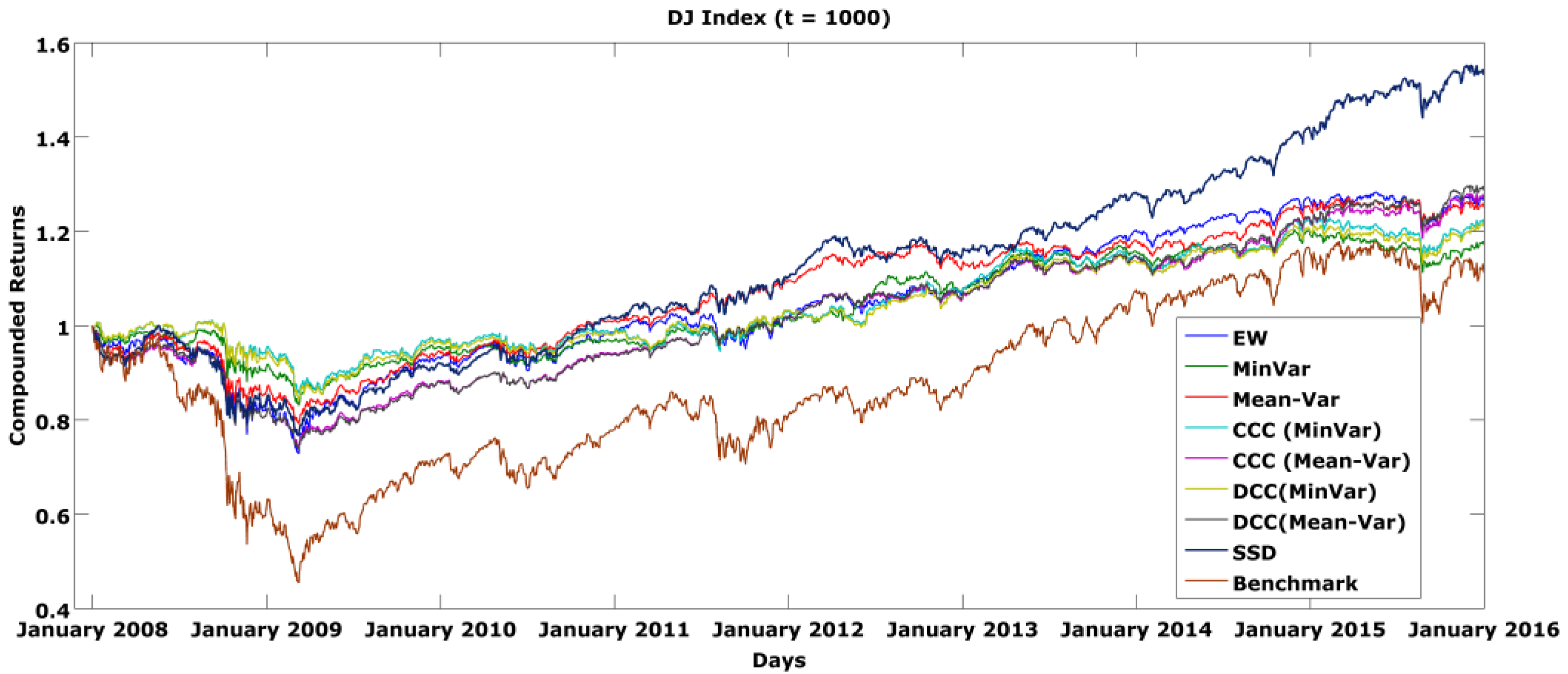
In Table 4 (DJ stocks, t = 1000), the SSD constrained portfolio has the highest T_R (1.5317) and Sh_R (0.9008).
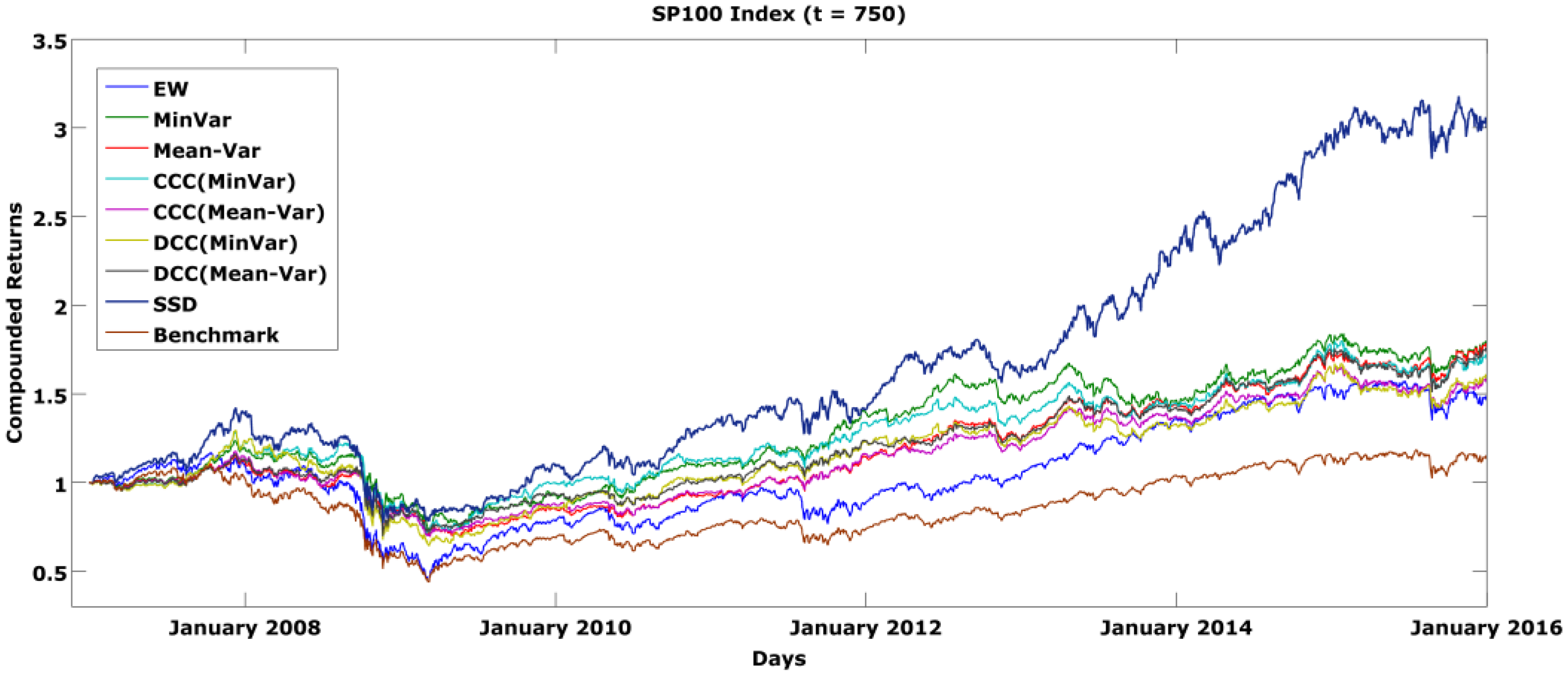
In Table 5 (S&P 100 stocks, t = 750), the SSD constrained portfolio has the highest T_R (3.0027) and Sh_R (0.9157).
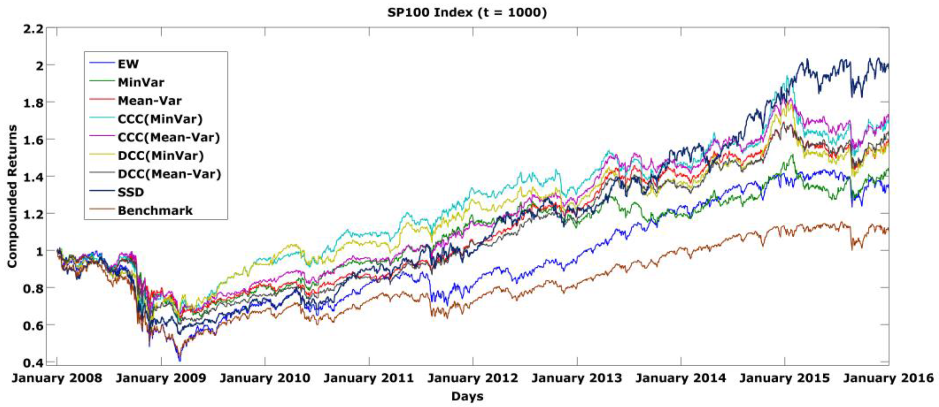
In Table 6 (S&P 100 stocks, t = 1000), the SSD constrained portfolio has the highest T_R (1.9756) and Sh_R (0.7110).
In 
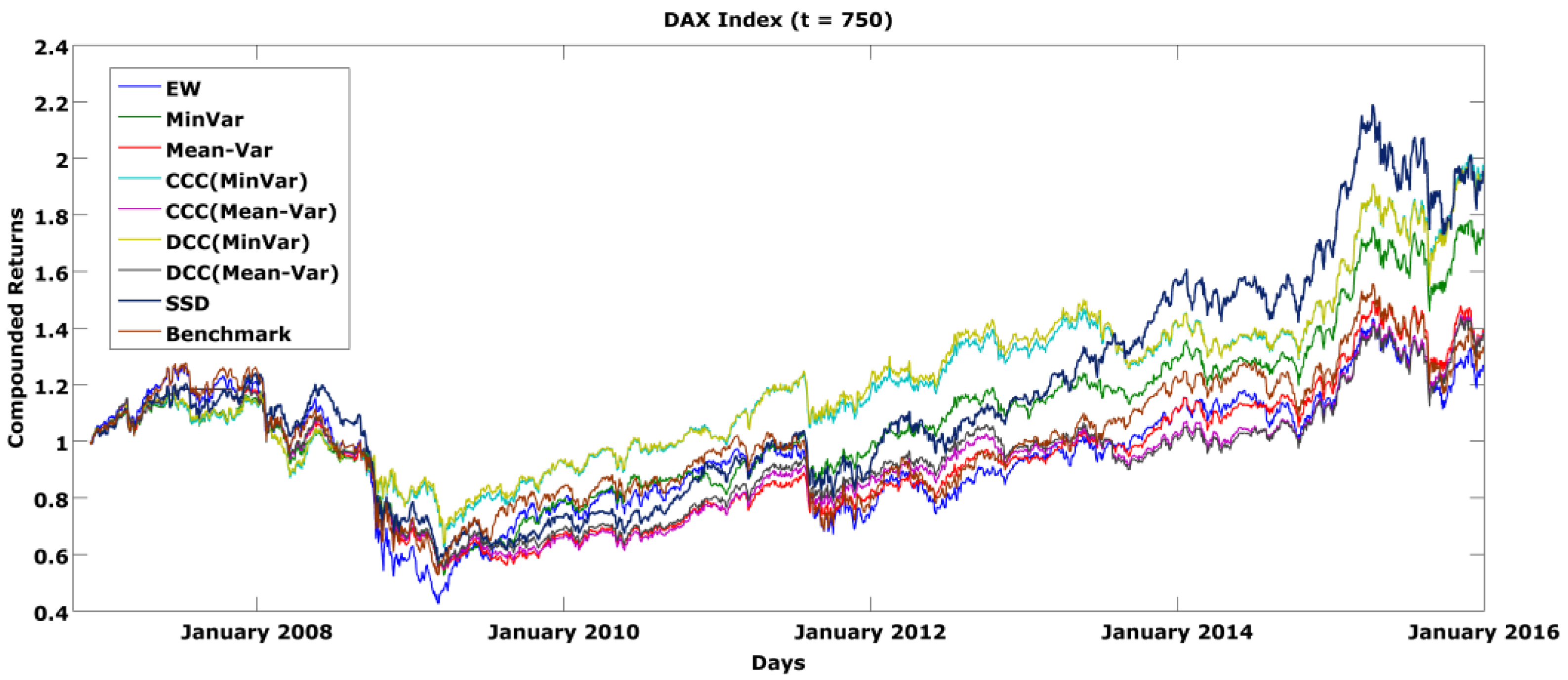
Table 7 (DAX stocks, t = 750), the SSD constrained portfolio has T_R (1.9364) higher than all considered portfolios, except CCC MinVar, and Sh_R (0.5164) higher than all considered portfolios, except CCC MinVar and DCC MinVar.
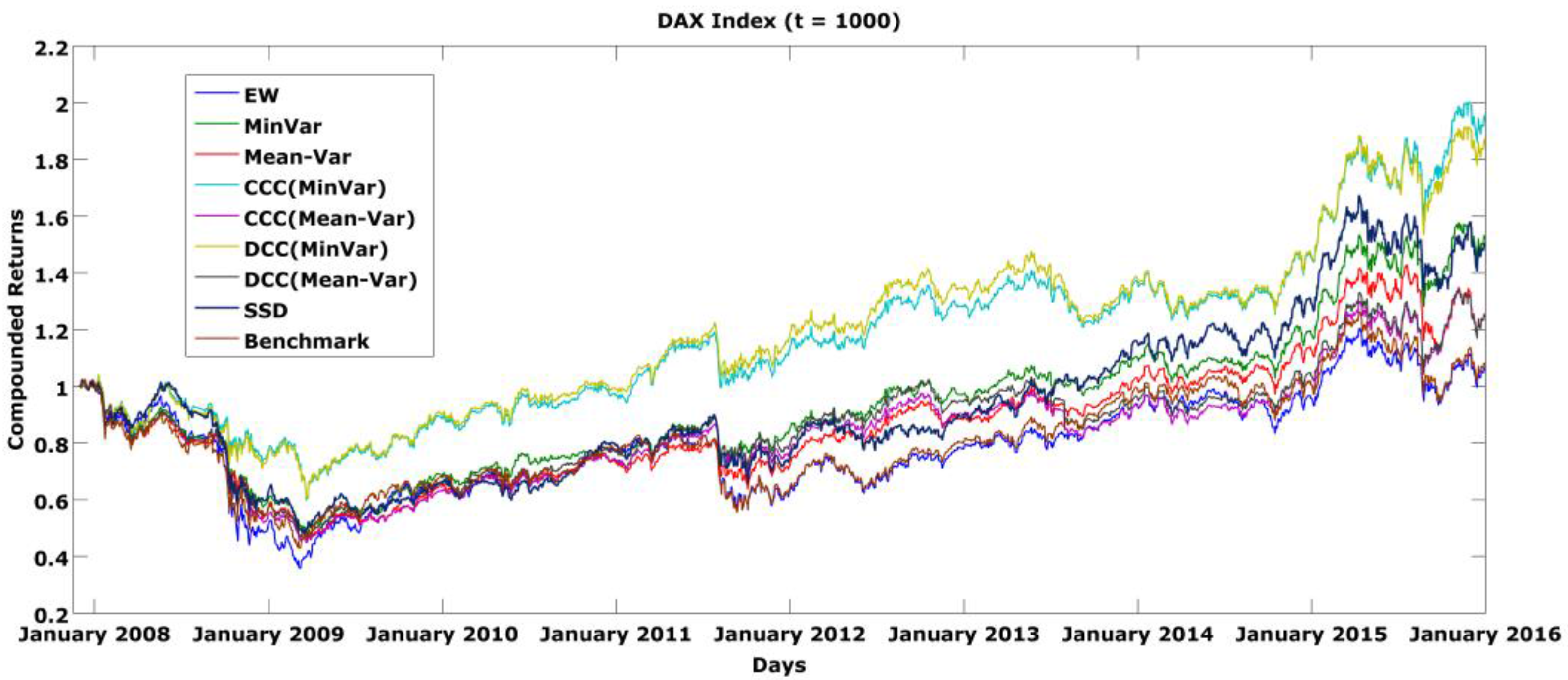
In Table 8 (DAX stocks, t = 1000), the SSD constrained portfolio has T_R (1.4897) and Sh_R (0.39520) higher than all considered portfolios, except MinVar, CCC MinVar and DCC MinVar.
Appendix A shows the weights of SSD constrained portfolios at the last month of the out-of-sample period and portfolio weights with all in-sample data. Appendix B shows company codes and names for the Dow Jones, SP500 and DAX indices.

4. Conclusions

This paper used Portfolio Safeguard (PSG) for portfolio optimization with SSD constraints. The algorithms are very efficient and can be run on a regular PC. The index portfolio optimization instances have 3046, 3020 and 3020 scenarios (daily returns) and 26, 29 and 90 variables, accordingly. The solution times are 0.27, 0.05 and 0.21 s for these instances. Another instance with 76 variables and 972 scenarios was optimized during 1.4 s. We have done out-of-sample simulations and compared SSD constrained portfolios with the minimum variance and mean-variance portfolios. The portfolios were constructed from the stocks of the DJ, S&P 100 and DAX indices. The SSD constrained portfolio demonstrated quite good out-of-sample performance and in the majority of cases had the highest compounded return and Sharpe ratio (among the considered portfolios). We think that SSD constrained optimization can be widely used in actual portfolio management, similar to mean-variance optimization.

Author Contributions

N. Fidan Keçeci wrote the paper and conducted the case study. V. Kuzmenko was involved in proving mathematical statements and in software development for the case study. S. Uryasev provided an overall guidance of the project.

Conflicts of Interest

The authors declare no conflict of interest.

Appendix A

Table A1. Weights of SSD constrained portfolios at the last month of the out-of-sample period and weights with all in-sample data. Stocks with zero positions for all periods (750, 1000 and 3020 days for DJ and S&P 100 and 750, 1000 and 3046 days for DAX) are skipped.
DJWeightsS&P 100WeightsDAXWeights
Code750 Days1000 days3020 DaysCODE750 Days1000 Days3020 DaysCode750 Days1000 Days3046 Days
AAPL000.2AAPL000.2ADS.DE000.075
DIS0.20.20.2ALL00.0280ALV.DE00.05550
HD0.20.20.2AMZN0.0210.0160.031BAYN.DE00.0660.2
MCD000.2BIIB000.086CON.DE0.20.20.2
MSFT0.20.20BMY0.01600DAI.DE0.0630.1320
NKE0.20.20.2CVS00.0040DB1.DE0.13700
UNH0.20.20DIS0.0860.1010DPW.DE00.20
GD0.04600DTE.DE0.200
GILD0.0630.1550.127FRE.DE0.20.20.2
HD0.0210.20SDF.DE000.125
LMT0.20.20.043IFX.DE0.200
LOW0.0010.0230MRK.DE00.14660.2
MCD000.113
MO0.1860.1720.2
MSFT0.05800
NKE0.20.0050.2
RTN0.0160.0960
SBUX0.04500
WBA0.04100

Appendix B

Table B1. DJ and DAX company codes and names.
DAXDJ
CodeNameCodeName
1EOAN.DEE.ON SEAAPLApple Inc.
2ADS.DEAdidas AGAXPAmerican Express Company
3ALV.DEAllianz SEBAThe Boeing Company
4BAS.DEBASF SECATCaterpillar Inc.
5BAYN.DEBayer AGCSCOCisco Systems, Inc.
6BEI.DEBeiersdorf AGCVXChevron Corporation
7BMW.DEBayerische Mot. Werke Aktienges.DDE. I. du Pont de Nemours and Company
8CBK.DECommerzbank AGDISThe Walt Disney Company
9CON.DEContinental AktiengesellschaftGEGeneral Electric Company
10DAI.DEDaimler AGGSThe Goldman Sachs Group, Inc.
11DB1.DEDeutsche Boerse AGHDThe Home Depot, Inc.
12DBK.DEDeutsche Bank AGIBMInt. Business Machines Corporation
13DPW.DEDeutsche Post AGINTCIntel Corporation
14DTE.DEDeutsche Telekom AGJNJJohnson & Johnson
15FME.DEFres. Med. Care AG & Co. KGAAJPMJPMorgan Chase & Co.
16FRE.DEFresenius SE & Co. KGaAKOThe Coca-Cola Company
17HEI.DEHeidelberg Cement AGMCDMcDonald’s Corp.
18SDF.DEK + S AktiengesellschaftMMM3M Company
19IFX.DEInfineon Technologies AGMRKMerck & Co. Inc.
20LHA.DEDeutsche Luft. AktiengesellschaftMSFTMicrosoft Corporation
21LIN.DELinde AktiengesellschaftNKENike, Inc.
22MRK.DEMerck KGaAPFEPfizer Inc.
23MUV2.DEMünchener R.G.A.PGThe Procter & Gamble Company
24SAP.DESAP SETRVThe Travelers Companies, Inc.
25SIE.DESiemens AktiengesellschaftUNHUnitedHealth Group Incorporated
26TKA.DEThyssenKrupp AGUTXUnited Technologies Corporation
27 VZVerizon Communications Inc.
28 WMTWal-Mart Stores Inc.
29 XOMExxon Mobil Corporation
Table B2. S&P 100 company codes and names.
CodeNameCodeName
1AAPLApple Inc.IBMInternational Business Machines
2ABTAbbott LaboratoriesINTCIntel Corporation
3ACNAccenture plcJNJJohnson & Johnson Inc.
4AIGAmerican International Group Inc.JPMJP Morgan Chase & Co
5ALLAllstate Corp.KOThe Coca-Cola Company
6AMGNAmgen Inc.LLYEli Lilly and Company
7AMZNAmazon.comLMTLockheed-Martin
8APAApache Corp.LOWLowe’s
9APCAnadarko Petroleum Corp.MCDMcDonald’s Corp.
10AXPAmerican Express Inc.MDLZMondelēz International
11BABoeing Co.MDTMedtronic Inc.
12BACBank of America CorpMETMetLife Inc.
13BAXBaxter International Inc.MMM3M Company
14BIIBBiogen IdecMOAltria Group
15BKBank of New YorkMONMonsanto
16BMYBristol-Myers SquibbMRKMerck & Co.
17BRK.BBerkshire HathawayMSMorgan Stanley
18CCitigroup Inc.MSFTMicrosoft
19CATCaterpillar Inc.NKENike
20CLColgate-Palmolive Co.NOVNational Oilwell Varco
21CMCSAComcast CorporationORCLOracle Corporation
22COFCapital One Financial Corp.OXYOccidental Petroleum Corp.
23COPConocoPhillipsPEPPepsiCo Inc.
24COSTCostcoPFEPfizer Inc.
25CSCOCisco SystemsPGProcter & Gamble Co
26CVSCVS CaremarkQCOMQualcomm Inc.
27CVXChevronRTNRaytheon Company
28DDDuPontSBUXStarbucks Corporation
29DISThe Walt Disney CompanySLBSchlumberger
30DOWDow ChemicalSOSouthern Company
21EBAYeBay Inc.SPGSimon Property Group, Inc.
32EMCEMC CorporationTAT&T Inc.
33EMREmerson Electric Co.TGTTarget Corp.
34EXCExelonTWXTime Warner Inc.
35FFord MotorTXNTexas Instruments
36FCXFreeport-McMoranUNHUnitedHealth Group Inc.
37FDXFedExUNPUnion Pacific Corp.
38FOXATwenty-First Century Fox, Inc.UPSUnited Parcel Service Inc.
39GDGeneral DynamicsUSBUS Bancorp
40GEGeneral Electric Co.UTXUnited Technologies Corp
41GILDGilead SciencesVZVerizon Communications Inc.
42GSGoldman SachsWBAWalgreens Boots Alliance
43HALHalliburtonWFCWells Fargo
44HDHome DepotWMTWal-Mart
45HONHoneywellXOMExxon Mobil Corp

References

  1. H. Markowitz. “Portfolio Selection.” J. Financ. 7 (1952): 77–91. [Google Scholar] [CrossRef]
  2. H.B. Mann, and D.R. Whitney. “On a Test of Whether one of Two Random Variables is Stochastically Larger than the Other.” Ann. Math. Stat. 18 (1947): 50–60. [Google Scholar] [CrossRef]
  3. E.L. Lehmann. “Ordered Families of Distributions.” Ann. Math. Stat. 26 (1955): 399–419. [Google Scholar] [CrossRef]
  4. H. Levy. Stochastic Dominance: Investment Decision Making under Uncertainty. Berlin, Germany: Springer, 2015. [Google Scholar]
  5. A. Muller, and D. Stoyan. Comparison Methods for Stochastic Models and Risks. Chichester, UK: John Wiley & Sons, 2002. [Google Scholar]
  6. M. Shaked, and J.G. Shanthikumar. Stochastic Orders and Their Applications. Boston, MA, USA: Academic Press, 1994. [Google Scholar]
  7. G.A. Whitmore, and M.C. Findlay, eds. Stochastic Dominance: An Approach to Decision-Making Under Risk. Lanham, MD, USA: Lexington Books, 1978.
  8. A. Lizyayev. “Stochastic dominance efficiency analysis of diversified portfolios: Classification, comparison and refinements.” Ann. Oper. Res. 196 (2012): 391–410. [Google Scholar] [CrossRef]
  9. W. Ogryczak, and A. Ruszczynski. “Dual Stochastic Dominance and Related Mean-Risk Models.” SIAM J. Optim. 13 (2002): 60–78. [Google Scholar] [CrossRef]
  10. D. Dentcheva, and A. Ruszczynski. “Optimization with Stochastic Dominance Constraints.” SIAM J. Optim. 14 (2003): 548–566. [Google Scholar] [CrossRef]
  11. T. Kuosmanen. “Efficient Diversification According to Stochastic Dominance Criteria.” Manag. Sci. 50 (2004): 1390–1406. [Google Scholar] [CrossRef]
  12. D. Dentcheva, and A. Ruszczynski. “Portfolio optimization with stochastic dominance constraints.” J. Bank. Financ. 30 (2006): 433–451. [Google Scholar] [CrossRef]
  13. G. Rudolf, and A. Ruszczynski. “Optimization Problems with Second Order Stochastic Dominance Constraints: Duality, Compact Formulations, and Cut Generation Methods.” SIAM J. Optim. 19 (2008): 1326–1343. [Google Scholar] [CrossRef]
  14. D. Dentcheva, and A. Ruszczynski. “Inverse stochastic dominance constraints and rank dependent expected utility theory.” Math. Program. 108 (2006): 297–311. [Google Scholar] [CrossRef]
  15. M. Kopa, and P. Chovanec. “A second-order stochastic dominance portfolio efficiency measure.” Kybernetika 44 (2008): 243–258. [Google Scholar]
  16. D. Dentcheva, and A. Ruszczynski. “Inverse cutting plane methods for optimization problems with second-order stochastic dominance constraints.” Optimization 59 (2010): 323–338. [Google Scholar] [CrossRef]
  17. D. Roman, K. Darby-Dowman, and G. Mitra. “Portfolio construction based on stochastic dominance and target return distributions.” Math. Program. Ser. B 108 (2006): 541–569. [Google Scholar] [CrossRef]
  18. C.I. Fabian, G. Mitra, D. Roman, and V. Zverovich. “An enhanced model for portfolio choice with SSD criteria: A constructive approach.” Quant. Financ. 11 (2011): 1525–1534. [Google Scholar] [CrossRef]
  19. C.I. Fabian, G. Mitra, and D. Roman. “Processing second-order stochastic dominance models using cutting-plane representations.” Math. Program. 130 (2011): 33–57. [Google Scholar] [CrossRef]
  20. American Optimal Decisions, Inc. “Portfolio Safeguard (PSG).” Available online: http://aorda.com/index.php/portfolio-safeguard/ (accessed on 31 December 2015).
  21. W. Ogryczak, and A. Ruszczynski. “From stochastic dominance to mean-risk models: Semideviations as risk measures.” Eur. J. Oper. Res. 116 (1999): 33–50. [Google Scholar] [CrossRef]
  22. “Case Study: Portfolio Optimization with Second-Order Stochastic Dominance Constraints.” Available online: http://www.ise.ufl.edu/uryasev/research/testproblems/financial_engineering/portfolio-optimization-with-second-orders-stochastic-dominance-constraints/ (accessed on 17 August 2016).
  23. Yahoo! “Finance.” Available online: https://www.finance.yahoo.com (accessed on 31 December 2015).
  24. MATLAB R2012b, Natick, Massachusetts, United States: The MathWorks, Inc., 2012.
  25. R.F. Engle, and K. Sheppard. Theoretical and Empirical Properties of Dynamic Conditional Correlation Multivariate GARCH. NBER Working Paper No. w8554; Cambridge, MA, USA: National Bureau of Economic Research, 2001. [Google Scholar]
  26. C. He, and T. Terasvirta. “An Extended Constant Conditional Correlation GARCH Model and Its Fourth-Moment Structure.” Econom. Theory 20 (2004): 904–926. [Google Scholar] [CrossRef]
  27. Y.K. Tse, and A.K.C. Tsui. “A Multivariate Generalized Autoregressive Conditional Heteroscedasticity Model with TimeVarying Correlations.” J. Bus. Econ. Stat. 20 (2002): 351–362. [Google Scholar] [CrossRef]
  28. R. Engle. “Dynamic Conditional Correlation: A Simple Class of Multivariate Generalized Autoregressive Conditional Heteroskedasticity Models.” J. Bus. Econ. Stat. 20 (2002): 339–350. [Google Scholar] [CrossRef]
  29. L. Bauwens, S. Laurent, and J.V. Rombouts. “Multivariate GARCH models: A survey.” J. Appl. Economy. 21 (2006): 79–109. [Google Scholar] [CrossRef]
  30. C. Alexander. Market Risk Analysis: Practical Financial Econometrics. Hoboken, NJ, USA: John Willey & Sons, 2008. [Google Scholar]
  31. “Kevin Sheppard Oxford-Man Institute of Quantitative Finance, Oxford, U.K. MFE Toolbox.” Available online: https://www.kevinsheppard.com/MFE_Toolbox (accessed on 12 October 2015).
  • 1American Optimal Decision (www.aorda.com), Gainesville, FL 32611, USA.
  • 2Deutsche Boerse AG (DB1.DE), Fresenius SE & Co. KGaA (FRE.DE), Infineon Technologies AG (IFX.DE) and Merck & Co. (MRK.DE) stock prices are adjusted for splits.
  • 3The CCC-GARCH and DCC-GARCH models are estimated by using MFE Toolbox for MATLAB software produced by Kevin Sheppard.
Figure 1. Compounded (on daily basis) returns of portfolios consisting of DJ stocks, t = 750. CCC, Constant Conditional Correlation; DCC, Dynamic Conditional Correlation.
Jrfm 09 00011 g001
Figure 2. Compounded (on daily basis) returns of portfolios consisting of DJ stocks, t = 1000.
Jrfm 09 00011 g002
Figure 3. Compounded (on daily basis) returns of portfolios consisting of S&P 100 stocks, t = 750.
Jrfm 09 00011 g003
Figure 4. Compounded (on daily basis) returns of portfolios consisting of SP100 stocks, t = 1000.
Jrfm 09 00011 g004
Figure 5. Compounded (on daily basis) returns of portfolios consisting of DAX stocks, t = 750.
Jrfm 09 00011 g005
Figure 6. Compounded (on daily basis) returns of portfolios consisting of DAX stocks, t = 1000.
Jrfm 09 00011 g006
Table 1. Expected yearly returns of portfolios. EW, Equally Weighted; MinVar, Minimum Variance; Mean-Var, Mean-Variance; SSD, Second-Order Stochastic Dominance.
PortfoliosDJIS&P 100DAX
EW0.040140.085090.09139
MinVar0.034190.087950.13362
Mean-Var0.083270.083270.08327
SSD0.087620.242500.17922
Benchmark0.043740.042870.08439
Table 2. Loading and solving times (in seconds) with PSG in the MATLAB environment.
DJIS&P 100DAX
ProblemLoadingSolvingLoadingSolvingLoadingSolving
SSD constrained (PSG code)2.110.121.390.191.800.11
MinVar (PSG riskprog)0.270.010.330.010.260.01
Mean-Var (PSG riskprog)0.380.010.440.020.380.01
Table 3. Yearly compounded returns, Total compounded Return (T_R) and Sharpe Ratio (Sh_R) for DJ stocks (t = 750).
Portfolios200720082009201020112012201320142015TRSh_R
EW1.05140.83221.11661.06111.02801.05611.12431.05011.00101.33000.5398
MinVar1.07120.91691.04451.01471.05491.04331.07641.02530.99321.25570.4736
Mean-Var1.06660.83441.06001.05651.07761.03931.04981.07281.0161.27710.5303
CCC MinVar1.0740.92850.99711.00851.05851.02951.07251.04291.01161.23630.4230
CCC Mean-Var1.08050.83121.04991.05571.07421.03611.0581.07221.05451.32520.5801
DCC MinVar1.07550.92091.01741.00761.06801.03101.07101.04751.01451.27250.4977
DCC Mean-Var1.08140.83941.06231.05581.07851.03731.06361.06901.05381.36490.6422
SSD1.12020.80231.08731.10371.01091.06401.08271.06661.04211.39610.5761
Benchmark1.05310.61571.15401.09581.03211.06521.25841.06880.96611.17150.1660
Table 4. Yearly compounded returns, Total compounded Return (T_R) and Sharpe Ratio (Sh_R) for DJ stocks (t = 1000).
Portfolios20082009201020112012201320142015TRSh_R
EW0.83221.11661.06111.02801.05611.12431.05011.00101.26500.4948
MinVar0.91321.04241.01621.04951.05831.07731.03090.98211.17190.3458
Mean-Var0.86141.09301.07241.08321.02781.05121.05641.00211.25090.5384
CCC MinVar0.95151.01681.01841.04441.04271.07001.05921.00061.21690.4356
CCC Mean-Var0.81291.08241.06921.08081.03821.08741.06571.03751.26920.5521
DCC MinVar0.94031.02361.01981.05131.02721.07191.05681.00751.20970.4303
DCC Mean-Var0.81341.07911.06951.08401.04091.08481.06711.04941.28660.5785
SSD0.84161.09141.10571.08481.04491.11491.10131.08361.53170.9008
Benchmark0.61571.15401.09581.03211.06521.25841.06880.96611.11240.1325
Table 5. Yearly compounded returns, Total compounded Return (T_R) and Sharpe Ratio (Sh_R) for S&P 100 stocks (t = 750).
Portfolios200720082009201020112012201320142015TRSh_R
EW1.09740.57951.22851.14900.97991.17361.32121.12180.95661.46330.3491
MinVar1.19680.77121.00441.19321.26491.04151.00661.22320.98821.77280.5230
Mean-Var1.11940.76860.98461.09791.23061.08741.15951.17581.03651.75880.5944
CCC MinVar1.23490.71551.12411.13931.17961.00301.08361.20310.97201.69660.4367
CCC Mean-Var1.14550.73691.03231.08611.22631.02461.15611.18120.96341.56440.4227
DCC MinVar1.23970.63301.09041.19721.19680.99361.09281.21680.97821.58440.3940
DCC Mean-Var1.12890.73631.11771.09271.21641.00401.14801.20901.00621.73120.5401
SSD1.39030.61631.27211.20171.07691.14891.43821.25421.02703.00270.9157
Benchmark1.02550.58031.15321.08460.98391.12401.26671.09580.99081.13190.1342
Table 6. Yearly compounded returns, Total compounded Return (T_R) and Sharpe Ratio (Sh_R) for S&P 100 stocks (t = 1000).
Portfolios20082009201020112012201320142015TRSh_R
EW0.57951.22851.1490.97991.17361.32121.12180.95661.33350.3054
MinVar0.77041.04171.17241.25980.95271.06141.19610.99291.42330.3610
Mean-Var0.78821.02451.07861.21111.12921.18721.16920.95131.57280.5141
CCC MinVar0.75131.26391.14791.22040.98311.12871.2590.90491.68170.4441
CCC Mean-Var0.76791.08361.15251.20241.09011.16221.22410.95511.70790.5720
DCC MinVar0.70061.31411.131.21880.96471.12271.25690.9011.55510.3810
DCC Mean-Var0.70671.06911.13311.22361.10161.17081.22560.97581.61570.5068
SSD0.62251.17751.21891.10211.21941.28111.18091.08761.97560.7110
Benchmark0.58031.15321.08460.98391.1241.26671.09580.99081.10380.1231
Table 7. Yearly compounded returns, Total compounded Return (T_R) and Sharpe Ratio (Sh_R) for DAX stocks (t = 750).
Portfolios200720082009201020112012201320142015TRSh_R
EW1.14760.50031.28871.16870.81191.25261.20341.02171.10131.25820.1883
MinVar1.11950.58651.16081.07421.14871.15911.15371.06981.24791.73280.5114
Mean-Var1.14170.56970.99061.1521.05351.15991.19061.0751.15041.38240.3366
CCC MinVar1.10790.70951.13881.10071.14391.14571.06971.04521.31731.95580.6235
CCC Mean-Var1.13730.58820.95041.17631.11121.12421.07021.09141.21951.37290.3126
DCC MinVar1.11230.71851.12191.09651.18611.13461.04661.04291.30181.93580.6118
DCC Mean-Var1.13340.59930.97641.16611.10191.11051.04071.10021.22201.36850.2998
SSD1.21250.60670.96581.23350.99801.28001.36731.07851.14491.93640.5164
Benchmark1.20820.55551.18911.14110.81811.26711.24141.01231.06561.32130.2248
Table 8. Yearly compounded returns, Total compounded Return (T_R) and Sharpe Ratio (Sh_R) for DAX stocks (t = 1000).
Portfolios20082009201020112012201320142015TRSh_R
EW0.50031.28871.16870.81191.25261.20341.02171.10131.05610.0864
MinVar0.59591.1471.07141.1481.15411.13711.07471.27721.51770.4489
Mean-Var0.56741.13641.13330.97931.23331.16671.09711.10361.24780.2632
CCC MinVar0.76751.14491.09591.15871.14231.06781.06561.32611.93550.6753
CCC Mean-Var0.54291.15341.17251.03321.17961.03761.08021.23371.24470.2435
DCC MinVar0.75611.17861.10321.1831.15051.02811.06071.26191.85200.6315
DCC Mean-Var0.56881.15661.16471.02491.19961.01881.07921.19391.24270.2429
SSD0.61651.04761.21010.93541.20221.3021.12011.14831.48970.3952
Benchmark0.55551.18911.14110.81811.26711.24141.01231.06561.07180.1042

