
Decomposed Driving Factors of Carbon Emissions and Scenario Analyses of Low-Carbon Transformation in 2020 and 2030 for Zhejiang Province


1
Institute of Land Science and Property, School of Public Affairs, Zhejiang University, Hangzhou 310058, China
2
Laboratory of Rural-Urban Construction Land Economical and Intensive Use, Ministry of Land and Resources, Beijing 100812, China
3
Institute of Agricultural Remote Sensing and Information Technology Application, College of Environmental and Resource Sciences, Zhejiang University, Hangzhou 310058, China
4
School of Public Policy and Administration Department of Public Administration, Xi’an JiaoTong University, Xi’an 710049, China
*
Author to whom correspondence should be addressed.
Energies 2017, 10(11), 1747; https://doi.org/10.3390/en10111747
Submission received: 9 September 2017
/
Revised: 16 October 2017
/
Accepted: 26 October 2017
/
Published: 31 October 2017
(This article belongs to the Special Issue Lessons from the Evaluation of Existing Emission Trading Schemes)
Abstract
:Climate change has gained widespread attention, and the rapid growth of the economy in China has generated a considerable amount of carbon emissions. Zhejiang Province was selected as a study area. First, the energy-related carbon emissions from 2000 to 2014 were accounted for, and then the Logarithmic Mean Divisia Index (LMDI) decomposition model was applied to analyse the driving factors underlying the carbon emissions. Finally, three scenarios (inertia, comparative decoupling and absolute decoupling) for 2020 and 2030 were simulated based on the low-carbon city and Human Impact Population Affluence Technology (IPAT) models. The results showed (1) carbon emissions increased by 1.66 times from 2000 to 2014, and trends of carbon emissions were used to divide the study period into three phases (rapid, medium growth and slow decrease phases, with annual growth rates of 12.60%, 4.77% and −1.24%, respectively); (2) the energy intensity effect from 2000–2011 inhibited carbon emissions but was exceeded by the economic output effect, which increased emissions, whereas the energy intensity effect from 2011–2014 outweighed the economic output effect; (3) the scenario analyses revealed that both the comparative and absolute decoupling scenarios would remain consistent with the carbon emissions boundaries in 2020 and 2030, but the comparative decoupling scenario was more reasonable for sustainable development. In addition, appropriate design of emission trading scheme could help to achieve the comparative decoupling by financial incentives.
1. Introduction
Climate change has received widespread attention because it threatens human survival. Approximately 63% of the gaseous radiative force that contributes to climate change is carbon [1]; thus, most of the international community has prioritized reducing carbon emissions and promoting low-carbon economic transitions. The economic growth in many developing countries, such as China and India, has occurred via extensive, environmentally unfriendly practices that required considerable energy consumption. The rapid growth of the population and economy in China has been closely associated with the excessive consumption of fossil fuels and generated large amounts of carbon emissions that accounted for 23% of the global energy consumption and 23.4% of the global carbon emissions in 2014 [2]. Increasing attention and pressure has been drawn to the Chinese government regarding these large amounts of carbon emissions. As a result, at the United Nations Climate Change conference held in Copenhagen in 2009, China promised that by 2020, the carbon dioxide emissions per unit of gross domestic product (GDP) would decrease by 40–45% compared with those in 2005. In 2016, the Paris Climate Accord was signed, and the Chinese government promised that China’s carbon emissions would peak in 2030 and carbon dioxide emissions per unit GDP would decrease by 60–65% compared with those in 2005. In order to achieve these ambitious targets in the wake of steady economic growth, a balance and coordination must be struck between economic growth and emission reductions while achieving low-carbon cities. Thus, there is a focal point on determining sustainable development modes of ensuring rapid economic growth while reducing carbon emissions levels.
The key to developing polices that reduce carbon emissions is to analyse the influencing factors and driving mechanisms underlying changes in carbon emissions from the relationships between industrial structure and carbon emissions [1,3,4,5], transportation and carbon emissions [6,7,8,9,10], building forms and carbon emissions [11,12,13], urban planning and carbon emissions [14,15,16], etc. Economic growth and population scale contribute greatly to China’s carbon emissions [17]. Using the Autoregressive Distributed Lag (ARDL) method and Factor Decomposition Model (FDM), only a unidirectional Granger causality was observed between urbanization and energy consumption from 1978 to 2008 in China [18]. A time series approach was used to explore the relationships among GDP, energy consumption and carbon emissions, and energy use in the Gulf Cooperation Council countries [19], European Economic and Monetary Union (EMU) countries [20], Israel [21], and Association of Southeast Asian Nations (ASEAN)-6 countries [22]. Feng performed an analysis of five regions in China (Shanghai, Guangdong, Heilongjiang, Henan and Gansu) and found that before the reform and opening-up policy, the dominating driving forces underlying increases in carbon emissions had changed from the growth of the population (1963–1965), to the affluence of the population (1966–1975), to changes in industrial structure (1952–1957, 1958–1962 and 1976–1978), whereas, after 1978, emissions intensity began to slow down relative to carbon emissions growth [23]. Moreover, several studies have compared the differences between the influencing factors for carbon emissions in different Chinese regions: urbanization had a larger impact on carbon emissions in western China and economic growth led to a more obvious influence in eastern China [24]. Yu applied improved fuzzy clustering and Shapley value decomposition models and found that per capita, the added value of secondary industry was the main factor for carbon emissions growth in Shanxi Province, Jiangsu Province and Hubei Province, whereas population growth was the main factor in Beijing City [25]. Additionally, several studies have explored the emissions embodied in the trade between regions; for example, nearly one fourth of global carbon emissions have been related to production exported from countries; thus, international trade has been viewed as a potential area to lower global emissions, with overseas imports accounting for 29–39% of the carbon footprint (CF) in Australia [26] and 40% of the CF in Xiamen City, China [27]. In China, 48% of carbon emissions associated with goods consumed in Chongqing City and more than 70% of the carbon emissions associated with Beijing, Shanghai and Tianjin were generated outside of their city boundaries [28]. An analysis of China–U.S. trade [29], China–UK trade [30], China–Japan trade [31] and China–Australia trade [32] showed that China’s international trade has had significant effects on global carbon emissions.
Local low-carbon scenario creations have been forecast in several cities, such as in Kyoto [33], Bangkok [34] , Shanghai [35] and Beijing [36]. Scenario analysis is an effective method of simulating carbon emissions resulting from different technology processes and policies in the future, and this method could contribute to the creation of an appropriate pathway to low-carbon development. The scenario is a forecast of future situations based on the original state description and future policies, and it includes indicators of possible developmental trends to facilitate policy adjustments. Comparing scenario settings could provide for a deep analysis of possible states in different trends, which could provide decision-making references for the selection of future development opportunities. For example, Wang combined nonlinear grey multivariable models with scenario analyses to forecast carbon emissions related to fossil energy consumption from 2014 to 2020 in China in three schemes that showed economic growth at low, medium, and high speeds [37]; Chen used Human Impact Population Affluence Technology (IPAT) to predict carbon emissions and water consumption in Dalian City in 2020 under different industrial structure scenarios within low-carbon goals and water constraints, and the results indicated that carbon emissions in the scenario with high-output value would be lowered by 8.5% compared with that of the baseline scenario [38]; Mi applied a structural decomposition analysis (SDA) that was used to extend an IPAT model to explore the key drivers (population, efficiency, production structure, consumption patterns and consumption volume) of China’s carbon emissions changes from 2005 to 2012, and the results indicated that global financial crisis had influenced the determinants of Chinese carbon emissions changes largely [39]; Liimatainen used a Delphi method approach to forecast the carbon emissions of Finnish road freight transport in 2030 under six scenarios based on different levels of economic development and found that carbon emissions in the maximum reduction scenario would represent a decrease of 74% from the 2010 level [40]; and Wang used a Stochastic Impacts by Regression on Population, Affluence, and Technology (STIRPAT) model to discuss low-carbon development in Minhang District, Shanghai and found that the best scenario would be achieved under high rates of affluence growth and energy intensity reduction along with medium rates of population growth and urbanization levels [41].
Although several studies have forecast whether China or Chinese regions could achieve the target carbon reduction emissions in 2020 [42,43,44,45], few studies have compared emissions reduction scenarios in 2020 and 2030. In addition, most analyses of carbon emission scenarios have considered only the carbon emissions intensity reduction target (carbon emissions per unit GDP) and ignored other targets, such as the carbon emissions boundary. Moreover, carbon emissions research from a regional perspective is important and could promote the achievement of China’s reduction targets. In this study, Zhejiang Province was selected as an example, and the Logarithmic Mean Divisia Index (LMDI) decomposition model was applied to analyse the driving factors of total carbon emissions. The carbon emissions under the three scenarios for 2020 and 2030 were simulated based on the models of the low-carbon city and IPAT, and the per capita carbon emissions for the three scenarios were also discussed in relation to whether they could achieve the carbon emission boundaries for 2020 and 2030.
2. Methodology and Data
2.1. Study Area and Data Source
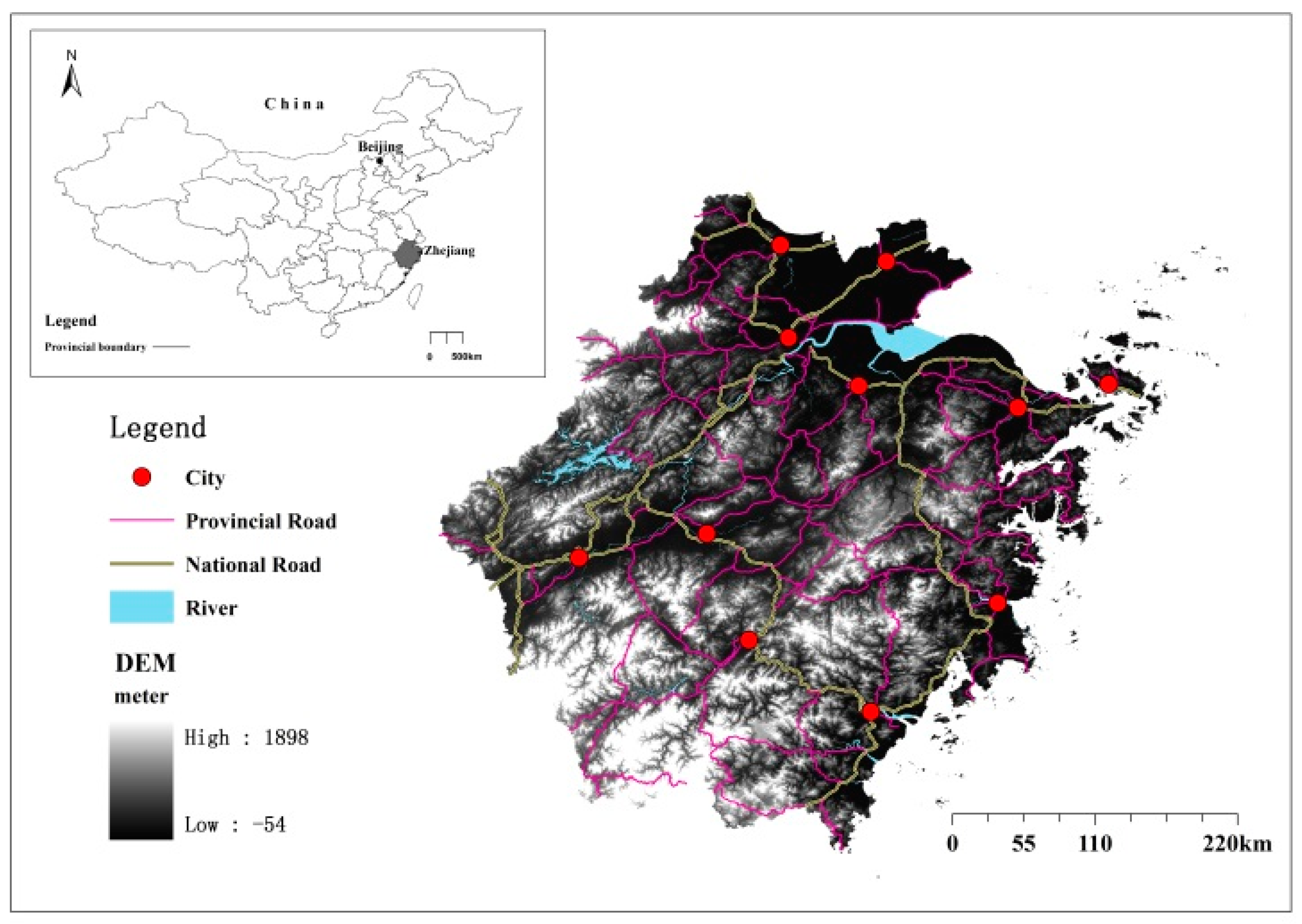
Located in the southeast coastal region of China (in Figure 1), the total land area of Zhejiang Province is 105,400 km2, and the province includes two sub-provincial cities (Hangzhou and Ningbo) and nine prefecture-level cities [46]. Zhejiang Province experienced rapid urbanization and industrialization at an urbanization rate of 64% in 2014, which has exceeded the national average by 11%. At the end of 2014, Zhejiang’s GDP per capita climbed to 73,312.81 yuan (approximately $11,825 USD), which was fourth among the 34 provincial-level administrative units in China.
However, such rapid urbanization and industrialization occurred at the expense of considerable resource consumption, such as fossil energy, which led to a high level of carbon emissions, thereby promoting global warming to a certain extent. The daily temperature in Zhejiang rose higher than 35 °C in 2001–2011 and increased by 8.49 days (in rural areas) and 12.01 days (in urban areas) compared with that of 1971–2000 [47]. With the promulgation of the National Medium and Long-Term Science and Technology Development Plan Outline of China (2006–2020) and the 13th Five-Year low-carbon development plan in the province of Zhejiang, the development of Zhejiang’s low-carbon city must be discussed.
Data on the population, GDP and primary energy consumption from 2000 to 2014 were collected from the Zhejiang Statistical Yearbooks and China Energy Statistical Yearbooks.
2.2. Estimation of Energy-Related Carbon Emissions
We calculated the carbon emissions of energy consumption based on the Intergovernmental Panel on Climate Change (IPCC ) Guidelines [48] as follows:
where Eitrepresents the ith type of fuel in the tth year and LCVi, CFit and Oi represent the lower calorific value, the carbon emissions factors, and the oxidation rate of fuel type i, respectively. The details of lower calorific value, carbon emissions factors and oxidation rate have been reported in previous literature [49,50].
2.3. IPAT and LMDI Decomposition Models
The IPAT model was reformulated as the Kaya identity, and it was first proposed by Ehrlich and Holdren [51] to analyse the environmental influence of different countries based on three key driving forces: population size (P), affluence (A, per capita consumption or production) and technology (T, impact per unit of economic activity, or all variations other than population and affluence). The IPCC also regarded this model as the basis for calculations, projections, and scenarios for greenhouse gases (GHGs) in 1996:
where I is the environmental load, P is the population, A is the affluence and T is the technology level. Based on the object of the study, the basic model is extended such that C (total carbon emissions) represents the environmental load indicator of I, P represents the total population size, G represents gross domestic product (GDP), E represents the total energy consumption; g represents the per capita GDP, e represents the energy structure and f represents the energy carbon intensity.
This model assumes that major changes in energy use technology do not occur in the short term and that carbon emission coefficients of each type of energy are relatively constant.
If C0 represents the carbon emission in the base year, the annual growth rate of GDP per capita is , the growth rate of population is , the rate of energy structure adjustment is , and the change rate of energy carbon intensity is , then the carbon emissions in target year (T) is as follows:
The LMDI originates from the Kaya identity [52], which explored the relationship between carbon emissions and population, GDP, and energy intensity. The Kaya identity was improved by the index decomposition analysis method and there was a large amount of research on the index decomposition method [53,54,55,56,57]. Compared with various index decomposition analyses, the LMDI method was deemed more appropriate because of its ease of use, adaptability, theoretical foundation and other desirable properties in the analysis [58].
The LMDI decomposition model is based on the extended Kaya decomposition method as follows:
where , , , and .
3. Results
3.1. Changes and Comparison of Carbon Emissions
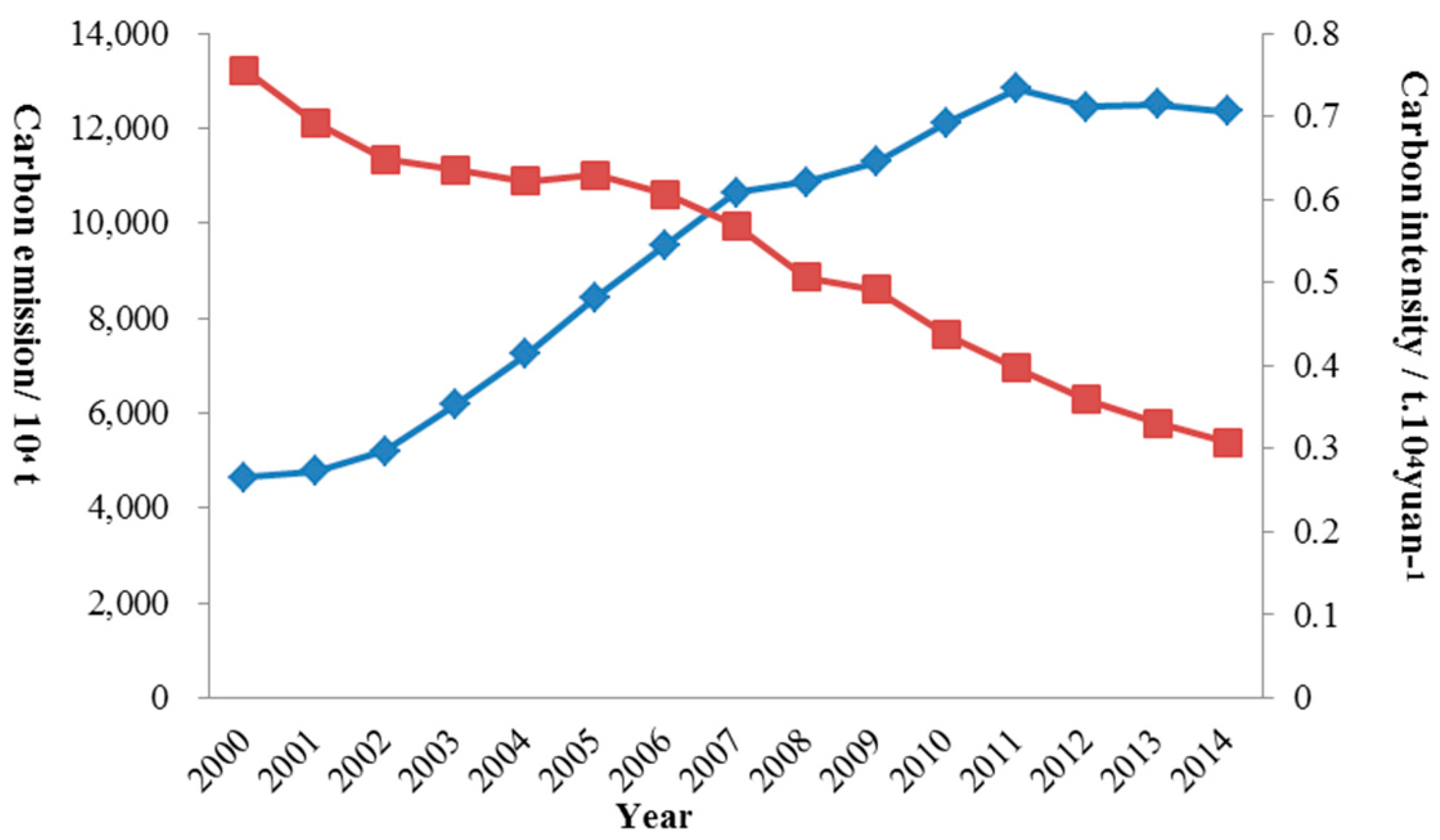
The changes in carbon emissions and carbon intensity (defined as the carbon emissions divided by GDP) are shown in Figure 2.
In the study period from 2000 to 2014, the total carbon emissions increased by 1.66 times, and the span can be divided into three phases (2000–2007, 2007–2011 and 2011–2014) according to the trends. In the first two periods, the carbon emissions tended to increase, although the annual growth rate varied between them, with carbon emissions presenting rapid growth in the first period at an annual growth rate of 12.60%, while the annual growth rate decreased in the second period to 4.77%. In the last period, the total carbon emissions began to show a decreasing trend, with the annual rate decreasing by 1.24%. Although the global financial crisis occurred in 2008, the total carbon emissions did not decrease immediately because the change in carbon emissions resulted from economic operations while social investments lagged behind. After 2011, the Zhejiang government promoted the strategic adjustment of the economic structure and stressed the quality of economic growth rather than its speed, which resulted in the decline of the total carbon emissions.
The carbon intensity decreased by 59.30% from 2000 to 2014 at an annual decreasing rate of 6.21%. Compared with the annual decreasing rate of other countries’ carbon emission intensities, Zhejiang’s annual rate was close to the annual declining rates in the emerging economy country of Brazil, which presented an annual declining rate of 5.09% [59], and it was much higher than that in certain industrialized countries, such as Britain (4.20%) and France (4.17%) during their most rapid declining rates in 10 years [59].
3.2. Influencing Factors for Carbon Emissions
The LMDI decomposition model was used to quantitatively analyse the factors influencing annual carbon emissions from 2000 to 2014 from the perspectives of economic growth, population size, energy intensity and energy structure (Table 1).
Economic output (GDP per capita) was the most important contributing factor, and it presented an incremental effect on the growth of carbon emissions in the study period. The accumulated effect reached 13,518.79 × 104 t and accounted for 175.08% of the change in total carbon emissions. GDP per capita increased by 4.56 times and total carbon emissions increased by 1.66 times, which indicated that economic growth was largely dependent on carbon emissions. The accumulation trend of the economic growth effect could be divided into three periods: 2000–2008, 2008–2011 and 2011–2014. From 2000 to 2008, the accumulation of the economic growth effect increased at an annual rate of 49.63%, which was much larger than that of the periods from 2008–2011 (13.17%) and 2011–2014 (3.68%). The investment scale in fixed assets in Zhejiang increased rapidly in the period from 2000–2008 at an annual increasing rate of more than 20%, thus exceeding the growth rate of GDP by a large margin. During this period, a large number of high energy consumption enterprises were placed into production and promoted energy consumption. Moreover, after China joined the WTO in 2001, Zhejiang Province entered a period of rapid industrialization, with the proportion of heavy industries showing a large increase from 45.99% in 2001 to 58.5% in 2008 and the development of heavy industries and their huge energy consumptions driving the rapid growth of carbon emissions. Due to the severe overcapacity of the industry, the growth rate of the per capita GDP in Zhejiang decreased sharply, resulting in a decrease of annual growth rate of accumulated economic growth effect.
In terms of the demographic effect, population growth had a positive effect on carbon emissions growth, although the incremental effect was less than that of per capita GDP. The accumulated demographic effect accounted for approximately 16.63% of the total carbon emissions. As population increases, carbon emissions grow rapidly because of increases in energy demand. According to Birdsall’s study [60], population and income growth leads to the additional consumption of resources and energy because of an increasing demand for goods and services. In addition, based on research and analyses of the migrant population of Zhejiang, the floating population in Zhejiang accounted for 21.7% of the entire resident population in 2010, 71.4% of which was young adults. Because of the relatively low educational level of these young adults, their primary areas of employment were dominated by secondary industries and service industries, which explained why the demographic changes had only an incremental effect on carbon emissions. In the process of urbanization in Zhejiang Province, the demographic trends included large-scale population migration from rural areas to big cities or from economically underdeveloped western China to Zhejiang Province. Thus, the demographic effect would have a large impact on carbon growth in Zhejiang and population growth must be controlled to maintain sustainable development.
The energy intensity effect was the most important factor for limiting carbon emissions increases, and the associated accumulated effects during the study period declined by 6945.77 × 104 t and accounted for approximately −89.95% of the total carbon emissions. Although the declining rate of the accumulated energy intensity effect slowed to 8.89% from 2008 to 2009, because of the global financial crisis, it recovered rapidly, which indicated that the energy-saving emissions reduction targets proposed by the 11th Five-Year plan and the energy saving and emission reduction plan of the 12th Five-Year had long-term influences on limiting carbon emissions via the adoption of more efficient energy use technologies and more advanced production technologies.
In terms of the energy structure effect, the accumulated impact of the energy structure effect on carbon emissions was unstable, and compared with that of the energy intensity effect, much weaker. These findings were related to Chinese energy consumption characteristics, which were dominated by coal; thus, limiting carbon emissions by optimizing the internal structures of fossil energy use was impossible in the short term. From 2001 to 2005, the energy structure effect had roughly inhibiting effects on carbon emission growth, which indicated that during a period of economic optimism, the government could promote energy use technologies and carbon emission reduction technologies to achieve energy alternatives, regardless of carbon emission growth. In addition, from 2006 to 2009, the energy structure had a positive effect on carbon emissions. The global economic crisis had an effect on China’s economic growth and technological progress, which led to the reuse of energy sources with high carbon emissions. After 2009, the energy structure effect presented an incremental effect on limiting the growth of carbon emissions, which reached a peak value at –135.41 × 10⁴ t in 2014, thus accounting for –1.75% of the total carbon emissions change.
3.3. Scenario Description and Simulation
3.3.1. Scenario Settings in 2020 and 2030
Inertia scenario: In this scenario, economic growth would still be the major target for social development, and the government would take measures for energy conservation and carbon emissions reduction sufficient to continue the present energy policy but without a stricter reduction policy than before. Thus, population growth, per capita GDP growth rate, energy intensity and energy structure coefficient would change annually at the average level for 2000–2014 by 1.17%, 13.21%, 6.04% and 1.22‰, respectively.
Comparative decoupling scenario: a low-carbon scenario under the integration of energy safety, sustainable development and low-carbon measures. In this scenario, economic growth would not be set as the primary target and the per capita GDP growth rate would drop to the level of 7.8%, which is less than the average level of the per capita GDP growth rate from 2010–2014 (8.8%). In addition, the energy intensity presented a phased corresponding change: from 2015 to 2020, it decreased annually by 6.5% through the low-carbon transformation of technology, and this rate was higher than the average level of change from 2000–2014 (6.04%); and from 2020 to 2030, its decreasing rate accelerated by 7.0%, which was higher than the level of change from 2013–2014 (6.52%). In addition, the average population growth reached 2% because of a universal two-child policy, and the energy structure coefficients reached the following targets: in 2020, non-fossil energy accounted for 20% of the primary energy, the proportion of coal consumption to primary energy consumption dropped to 42.8% and the proportion of natural gas consumption reached approximately 10%.
Absolute decoupling scenario: an enhanced low-carbon scenario in which the Zhejiang government makes active efforts to mitigate climate change in the last ten years of 2020 to 2030. From 2015 to 2020, the parameters were the same as that in the comparative decoupling scenario. However, from 2020 to 2030, the government will pay more attention to the transformation of economic development to a low-carbon mode at the expense of slowing down economic growth. Thus, we set the scenario indicators as follows: annual per capita GDP growth rate would drop to 4.50% if we assumed GDP growth at the low speed of 6.5%, which was the national bottom line in the 13th Five-Year. In addition, the average population growth remained at 2%, and the energy structure coefficient reached the following targets: in 2030, non-fossil energy accounted for 30% of the primary energy, the proportion of coal consumption to primary energy consumption dropped to 35% and the proportion of natural gas consumption reached approximately 15%.Table 2 lists the key variables considered in the analysis and used to highlight the scenario development: population growth rate, per capita GDP growth rate, energy intensity growth rate and energy structure growth rate. Table 2 shows the scenario settings for the carbon emissions of Zhejiang Province in 2020 and 2030. Chen and Zhu presented three aspects of theory as plans A, B and C [61]. Plan A is a historic way of development, where economic growth and urban development maintain the same pace as in traditional way and effective measures are not enacted to reduce emissions. Plan B is an ideal development mode that originates from Brown’s book [62]. In Plan B, economic growth is completely decoupled from carbon emission (which usually occurs when industrialization is completed and urbanization reaches a certain level with high living standards and social welfare) Plan C is the sustainable mode where carbon emissions would increase at first and then decrease [63]. Then, three scenarios are categorized further based on the elasticity coefficient between carbon emission and per capita GDP growth rate that is used to evaluate whether a city is developing on a low-carbon basis [61,64]: (1) For the inertia scenario of Plan A, the elasticity coefficient between carbon emissions growth and per capita GDP growth is more than 0.5. As for Zhejiang province, the average values of elasticity coefficient between carbon emissions growth and per capita GDP growth are 0.78 in the 10th Five-Year Plan period from 2001–2005 and 0.67 in the 11th Five-Year Plan period from 2006–2010; (2) for the comparative decoupling of Plan C, the elasticity coefficient is less than 0.5; and (3) for the absolute decoupling of Plan B, the elasticity coefficient is 0 or less than 0.
3.3.2. Scenario Simulation of Carbon Emission in 2020 and 2030
Three scenarios for carbon emissions in 2020 and 2030 are possible based on the IPAT model (in Table 2). In the inertia scenario, the rapid growth of carbon emissions would be driven by traditional extensive economic development, and the per capita GDP would reach 2.10 and 7.19 times that of the base year (2014). Moreover, in this scenario, the energy intensity decreased gradually (as it does historically) to 0.69 times and 0.37 times the value of the base years. As a result, the carbon emissions in the inertia scenario would be 1.35 times the value of those in the comparative decoupling and absolute decoupling scenarios by 2020 and 2.25 and 3.14 times the value of comparative decoupling and absolute decoupling scenarios by 2030, respectively. Economic growth in the comparative decoupling scenario was relatively slower than that in the inertia scenario and changed by 1.57 and 3.33 times the per capita GDP value of the base years in 2020 and 2030, respectively. In addition, the energy intensity rate would decrease more rapidly by 0.67 and 0.32 times that of the base year by 2020 and 2030, respectively. The industrial structure of Zhejiang is expected to be upgraded and the promotion of energy-saving industry would lead to gradual improvements. Compared with the comparative decoupling scenario, economic growth would be reduced by a large margin in the absolute decoupling scenario during the final period of 2020–2030. As a result, the per capita GDP would be 2.43 times that of the base year by 2030. In addition, carbon emissions in the comparative decoupling scenario would be 1.39 times the value of the absolute decoupling scenario by 2030.
In the inertia scenario, the carbon emissions in 2020 and 2030 would reach 1.54 times and 3.14 times that of 2014, reaching 19,038.41 × 104 t and 38,818.57 × 104 t, respectively. Carbon emissions would grow by 7.46% annually with an elasticity coefficient of 0.57. In the comparative decoupling scenario, Zhejiang’s carbon emissions reached their peak in 2030 and carbon emissions in 2020 and 2030 would be 1.14 times and 1.39 times that of 2014, reaching 14,093.37 × 104 t and 17,235.54 × 104 t. In this scenario, the carbon emissions growth would be controlled at an average rate of 2.21% with an elasticity coefficient of 0.28 from 2014–2020 and at an average rate of 2.03% with an elasticity coefficient of 0.26 from 2020–2030, indicating that it is a comparative decoupling scenario. The absolute decoupling scenario enacted higher requirements than the comparative decoupling scenario. In this scenario, during the period from 2020–2030, the government will adopt mandatory emissions reduction policies, and Zhejiang’s carbon emissions in 2030 will be at the same level as that in 2014, thus representing a decrease to 12,362.60 × 104 t. The elasticity coefficient for 2030 is less than 0, which belongs to the absolute decoupling scenario. The carbon emissions intensity dropped in all three scenarios, and in the inertia scenario, it would decrease to 0.31 tC/104 yuan and 0.17 tC/104 yuan by 2020 and 2030, respectively, thereby reducing the emissions intensity by 65.90% and 81.70% compared with the levels of 2005, respectively. Thus, for Zhejiang Province, China's emission reduction commitments (relative emission reductions of carbon intensity) in the Copenhagen of 40–45% could be easily realized by 2020 and that in Paris agreement of 60–65% could be realized by 2020. However, the carbon emissions boundary should be considered in any low-carbon plan. According to the Paris Agreement, increases of global temperature by 2050 are supposed to be controlled to within 2 degrees, better within 1.5 degrees. According to the estimate by Hoekstra and Wiedmann [65], the carbon emissions boundary will be approximately 18 × 109 and 25 × 109 t·a−1, and with global population growth from 7 billion to almost 10 billion in 2050, the per capita carbon emissions should be controlled to less than 2.5 t·a−1. In the inertia scenario, the per capita carbon emissions would reach 3.21 t·a−1 and 5.84 t·a−1 in 2020 and 2030, respectively, which far exceed the per capita carbon emissions boundary. The per carbon emissions boundary could be met in both the comparative decoupling scenario and absolute decoupling scenario: in the comparative decoupling scenario, the per capita carbon emission would increase to 2.27 t·a−1 in both 2020 and 2030, whereas in the absolute decoupling scenario, the per capita carbon emission would reach 1.62 in 2030.
4. Discussion
The results indicate that the economic output per capita GDP effect was the main factor that drove carbon emissions and the energy intensity effect was the main factor that inhibited carbon emissions, which was consistent with previous research. Rapid economic growth caused a rising demand for energy products, although economic growth could also contribute to decreasing energy intensity via industrial structure adjustments and cleaner technology development. Our study showed that, in Zhejiang Province from 2000 to 2011, the energy intensity effect inhibiting carbon emissions was exceeded by an economic output effect, which increased carbon emissions, whereas from 2011 to 2014, the driving effect of economic output effect on carbon emissions was outweighed by the curbing effects of energy intensity because the economic and technological development stage of the region determined whether the combined effect of energy intensity and economic output could reduce carbon emissions. Because Zhejiang is an important province in the manufacturing and export economy, its economic growth was highly dependent on foreign countries, and its degree of dependence on foreign countries was close to 70% in 2010, which resulted in the province being heavily affected by international economic prosperity and the supply and demand of the international market. After the international financial crisis, a forced mechanism and industry transfer opportunity occurred, which allowed Zhejiang Province to eliminate and transfer the relative surplus capacity of traditional industries and labour-intensive manufacturing industries through the domestic industry gradient to other provinces. Thus, improving the quality of economic development via a moderate economic growth rate and higher energy intensity and technological progress were key objectives. Moreover, energy structures had little effect on limiting carbon emissions because of the high proportion of coal consumption used during Zhejiang Province’s economic development (which was still more than 70% in 2014). It should be noted that the energy structure effects were positive for carbon emissions growth in 2003, which was related to the rapid increase of industrial output and demand for energy products as well as to the income growth of residents caused by the acceleration of urbanization in China after 2001. Such changes led to a high proportion of coal consumption. In addition, a forum on the development of strategic emerging industries convened by Premier Wen Jiabao in 2009 contributed to the development of advanced and new technology and the optimization of the energy structure. For example, several subsidies were provided to develop wind power and solar power projects. As a result, the energy structure effects limiting carbon emissions experienced a sharp increase after 2009, although this was relatively low compared with the energy intensity effect. However, industrial adjustments lagged behind the demand of economic development, which explains why the total carbon emissions decreased after 2011.
To study China’s Zhejiang Province more realistically, the analysis should be extended to 2030, which represents the government’s peak carbon emissions target. In addition, setting the parameters of the model is helpful for considering more policy factors, such as a universal two-child policy. Several studies have focused on whether China could achieve the carbon emissions reduction target (relative emission reductions for carbon intensity) of 40–45% by 2020, whereas few studies have discussed the emissions reduction target in 2030 and carbon emissions boundaries. In the inertia scenario, the carbon emission intensity in 2020 decreased by 65.90% compared with that in 2005, which exceeded the new reduction emission targets promised by Chinese government according to the Paris agreement; thus, its per capita carbon emissions outweighed the boundary. Therefore, this scenario does not represent an ideal development scenario. To some extent, future plans for energy conservation and emissions reductions should consider various carbon emission boundaries, such as the per capita boundary, urbanization level boundary and so forth. The absolute decoupling scenario which presented an obvious carbon emission reduction in 2030 compared with that of other scenarios was based on the rapid decrease of economic growth rate from 2020 to 2030, with a growth rate of GDP per capita below 5%. As a result, GDP per capita of Zhejiang province in the absolute decoupling scenario in 2030 (2.7 × 10⁴ dollar, $) would be far away from targets of Yangtze River Delta economic development in 2030 that would be close to current level of the most developed countries(4 × 10⁴ dollar, $). On the other hand, China’s economy is gradually developing under the stewardship of an authoritarian government and not a free-market one. According to the economic growth targets of 12th Five-Year (2011–2015) Plan and 13th Five-Year (2016–2020) Plan of Zhejiang province that set annual growth rates of GDP at 8% and 7.5%, a growth rate of GDP per capita below 5% in the absolute decoupling scenario may not reach the targets Zhejiang’s 14th (2021–2025) and 15th (2026–2030) Plan although these two plans had not been formulated by the government. Thus, the absolute decoupling scenario would not be adapted to the current stage of development in Zhejiang. As to the comparative decoupling scenario, GDP per capita of Zhejiang province in 2030 (3.7 × 10⁴ dollar, $) would be close to the current level of the most developed countries and economic growth would not decrease by a large margin. As a result, the process of modernization and urbanization would not be hindered in the comparative decoupling scenario.
Traditional emission reduction policies of administrative orders would put high pressure of emission reduction on enterprises and emission trading scheme could help to reduce the mitigation cost for the whole economy through market mechanism. Moreover, central and western regions that are less economically developed in China could benefit from selling the excessive emissions trading quotas to eastern regions and eastern regions could also have more space to develop urbanization and modernization further. Interprovincial emission reduction quota trading could be beneficial to all the provinces, but each province may acquire different benefit under different equity criteria. Zhou found that interprovincial emission reduction quota trading could decrease emission abatement cost by more than 40% and criteria of carbon emissions and population would be relatively fairer criteria [66]. Thus, China would consider an emission trading scheme as a cost-effective way to achieve low carbon targets in the future as well as a policy instrument to transfer wealth across regions. There have been seven pilots at provincial and city levels in China (Beijing, Tianjin, Shanghai, Chongqing, Hubei, Guangdong and Shenzhen) that cover a wide range of different economic circumstances and the forthcoming national emission trading scheme would be established in late 2017. Although Zhejiang isn’t a pilot, there are some specific advantages in establishing a mature carbon emission trading market: Zhejiang province, as a most developed region in China, has mature internet and e-commerce markets and an efficient administrative system, which are advantages in establishing a relatively mature carbon emission market in 2020 according to the Plan of Emissions Trading Scheme in Zhejiang Province [67]. Compared with an inertia scenario in our study, energy intensities in the both comparative and absolute decoupling scenario would decrease by a large margin in 2020 and 2030. Currently, Zhejiang's energy structure has been dominated by coal (52.4% in 2016). Efficiency improvement will play an important role in low carbonization because it is difficult to find more space for further substitution of coal and coking products. In addition, efficiency improvements could be motivated and competitiveness of manufacturers could be improved in turn by financial incentive through appropriate carbon trading. For example, carbon quotas could be bought from low-carbon emission industries by high-carbon emission industries, which would bring more development space for both of them. Guangdong ׳s carbon emission trading scheme indicates that more sectors involved in emissions trading scheme could reduce the GDP loss and increase the economic outputs compared to that without emission trade scenarios [68], which supports the idea that appropriate design of emission trading schemes are economically efficient ways for carbon mitigation in China. In addition, economic effects of emissions trading scheme would be largely dependent on economic growth. In a comparative decoupling scenario, GDP growth would be slower from 2020 to 2030, which may lead to more climates policy-induced welfare loss because 0.5 percentage points lower growth would cause welfare loss in 2030 by nearly 0.5 percentage points [69]. As a developing country, China’s social welfare still needs to be improved by economic development and economic growth is still the first priority currently.
Thus, the comparative decoupling scenario was relatively reasonable for low-carbon development in the future for Zhejiang Province. The elasticity ratios of our study were smaller when compared with that of Chen’s scenario simulation of Shanghai [61]. Chen designed the parameters based on the period from 2000–2009, whereas our study referenced variations in the indicators for the period of 2000–2014. The economic structure was greatly optimized and policies of energy conservation and emission reduction were implemented more strictly in the period from 2000–2014. For example, the State Council in China considered the energy-saving emissions reduction rates when evaluating the performance of local officials.
5. Conclusions
We applied the LMDI decomposition model to analyse the driving factors underlying the total carbon emissions in terms of the economic output effect, demographic effect, energy intensity effect and energy structure effects for the period of 2000 to 2014 in Zhejiang Province, China. We then simulated the carbon emissions under three scenarios (inertia, comparative decoupling and absolute decoupling) for 2020 and 2030 based on the low-carbon city and IPAT models and then discussed whether carbon emissions under the three scenarios exceeded the carbon emissions boundary:
- (1)
- Total carbon emissions increased by 1.66 times from 2000 to 2014, and this period can be divided into three phases according to the trends: 2000–2007, 2007–2011 and 2011–2014. In the first two periods, the carbon emission tended to increase, but the annual growth rate varied, with carbon emissions presenting a rapid growth trend from 2000–2007 at an annual growth rate of 12.60% and then showing a medium annual growth rate from 2007–2011 at 4.77%. In the last period from 2011–2014, the total carbon emissions began to show a slow decreasing trend at an annual rate of 1.24%.
- (2)
- The economic output effect of the per capita GDP was the main factor that drove carbon emissions, whereas energy intensity effect was the main factor that inhibited emissions. In the period from 2000–2011, the energy intensity effect inhibiting carbon emissions was exceeded by the economic output effect, which increased carbon emissions; in the period from 2011–2014, the driving impact on carbon emissions of economic output effect was outweighed by the inhibiting impact of the energy intensity effect.
- (3)
- The results of the scenario analyses show that the carbon emissions in the inertia scenario would be 1.35 times the value of that in the comparative decoupling and absolute decoupling scenarios by 2020, whereas it would be 2.25 and 3.14 times the value of comparative decoupling and absolute decoupling scenarios by 2030, respectively.
- (4)
- According to the carbon emission boundary proposed by Hoekstra and Wiedmann (per capita carbon emission should be controlled to less than 2.5 t·a−1), only the comparative decoupling scenario and the absolute decoupling scenario would achieve the carbon emissions boundaries in both 2020 and 2030. The scenario analysis revealed that although both China’s commitment of the Copenhagen emission reduction targets and the recent Paris agreement targets could be reached in the inertia scenario, the per capita carbon emissions would exceed the carbon emissions boundary. Moreover, the comparative decoupling scenario was more reasonable than the absolute decoupling scenario because the latter scenario would delay the process of modernization and urbanization in Zhejiang. Appropriate design of emissions trading schemes could help to achieve the comparative decoupling scenario through motivating efficiency improvements and improving competitiveness of manufacturers in turn by financial incentives.
Acknowledgments
We thank the following for their financial support for this project: the National Key Research and Development Program of China (Grant No. 2016YFD0201200); the National Natural Science Foundation of China (Grant No. 41771244); the key project of Zhejiang Provincial Education Department (Z201121260); and the Fundamental Research Funds for the Central Universities.
Author Contributions
Yan Li developed the original idea and contributed to the conceptual framework. Yan Li and Chuyu Xia wrote the paper and were responsible for data collection, process and analysis. Yanmei Ye, Zhou Shi and Jingming Liu provided guidance and improving suggestions. All authors have read and approved the final manuscript.
Conflicts of Interest
The authors declare no conflict of interest.
References
- Wang, Q.; Li, R.; Jiang, R. Decoupling and Decomposition Analysis of Carbon Emissions from Industry: A Case Study from China. Sustainability 2016, 8, 1059. [Google Scholar] [CrossRef]
- BP Statistical Review of World Energy Market. Available online: http://www.bp.com/content/dam/bp/pdf/energy-economics/statistical-review-2015/bpstatistical-review-of-world-energy-2015-full-report.pdf (accessed on 14 June 2016).
- Zhang, X.; Zhao, Y.; Sun, Q.; Wang, C. Decomposition and Attribution Analysis of Industrial Carbon Intensity Changes in Xinjiang, China. Sustainability 2017, 9, 459. [Google Scholar] [CrossRef]
- Wang, S.; Li, Q.; Fang, C.; Zhou, C. The relationship between economic growth, energy consumption, and CO2 emissions: Empirical evidence from China. Sci. Total Environ. 2016, 542, 360–371. [Google Scholar] [CrossRef] [PubMed]
- Wu, R.; Zhang, J.; Bao, Y.; Lai, Q.; Tong, S.; Song, Y. Decomposing the Influencing Factors of Industrial Sector Carbon Dioxide Emissions in Inner Mongolia Based on the LMDI Method. Sustainability 2016, 8, 661. [Google Scholar] [CrossRef]
- Zhu, X.; Li, R. An Analysis of Decoupling and Influencing Factors of Carbon Emissions from the Transportation Sector in the Beijing-Tianjin-Hebei Area, China. Sustainability 2017, 9, 722. [Google Scholar] [CrossRef]
- Dong, J.; Deng, C.; Li, R.; Huang, J. Moving Low-Carbon Transportation in Xinjiang: Evidence from STIRPAT and Rigid Regression Models. Sustainability 2016, 9, 24. [Google Scholar] [CrossRef]
- Andrade, C.E.S.D.; D’Agosto, M.D.A. The Role of Rail Transit Systems in Reducing Energy and Carbon Dioxide Emissions: The Case of The City of Rio de Janeiro. Sustainability 2016, 8, 150. [Google Scholar] [CrossRef]
- Wright, L.; Fulton, L. Climate change mitigation and transport in developing nations. Transp. Rev. 2005, 25, 691–717. [Google Scholar] [CrossRef]
- He, D.; Meng, F.; Wang, M.Q.; He, K. Impacts of urban transportation mode split on CO2 emissions in Jinan, China. Energies 2011, 4, 685–699. [Google Scholar] [CrossRef]
- Hirokawa, K.H.; Pohrib, A.M. The Role of Green Building in Climate Change Adaptation. In Research Handbook On Climate Adaptation Law; Albany Law School: New York, NY, USA, 2012. [Google Scholar]
- Sun, B.; Luh, P.B.; Jia, Q.-S.; Jiang, Z.; Wang, F.; Song, C. Building energy management: Integrated control of active and passive heating, cooling, lighting, shading, and ventilation systems. IEEE Trans. Autom. Sci. Eng. 2013, 10, 588–602. [Google Scholar] [CrossRef]
- Xu, P.; Chan, E.H. ANP model for sustainable Building Energy Efficiency Retrofit (BEER) using Energy Performance Contracting (EPC) for hotel buildings in China. Habitat Int. 2013, 37, 104–112. [Google Scholar] [CrossRef]
- Ho, C.S.; Matsuoka, Y.; Simson, J.; Gomi, K. Low carbon urban development strategy in Malaysia—The case of Iskandar Malaysia development corridor. Habitat Int. 2013, 37, 43–51. [Google Scholar] [CrossRef] [Green Version]
- Fong, W.K.; Matsumoto, H.; Ho, C.S.; Lun, Y.F. Energy consumption and carbon dioxide emission considerations in the urban planning process in Malaysia. Plan. Malays. J. 2008, 6, 99–123. [Google Scholar]
- Lehmann, S.; Zaman, A.U.; Devlin, J.; Holyoak, N. Supporting urban planning of low-carbon precincts: Integrated demand forecasting. Sustainability 2013, 5, 5289–5318. [Google Scholar] [CrossRef]
- Wang, F.; Wang, C.; Su, Y.; Jin, L.; Wang, Y.; Zhang, X. Decomposition Analysis of Carbon Emission Factors from Energy Consumption in Guangdong Province from 1990 to 2014. Sustainability 2017, 9, 274. [Google Scholar] [CrossRef]
- Liu, Y. Exploring the relationship between urbanization and energy consumption in China using ARDL (autoregressive distributed lag) and FDM (factor decomposition model). Energy 2009, 34, 1846–1854. [Google Scholar] [CrossRef]
- Magazzino, C. The relationship between real GDP, CO2 emissions, and energy use in the GCC countries: A time series approach. Cogent Econ. Financ. 2016, 4, 1152729. [Google Scholar] [CrossRef]
- Magazzino, C. Is per capita energy use stationary? Panel data evidence for the EMU countries. Energy Explor. Exploit. 2016, 34, 440–448. [Google Scholar] [CrossRef]
- Magazzino, C. Economic growth, CO2 emissions and energy use in Israel. Int. J. Sustain. Dev. World Ecol. 2015, 22, 89–97. [Google Scholar] [CrossRef]
- Magazzino, C. A panel VAR approach of the relationship among economic growth, CO2 emissions, and energy use in the ASEAN-6 countries. Int. J. Energy Econ. Policy 2014, 4, 546–553. [Google Scholar]
- Feng, K.; Hubacek, K.; Guan, D. Lifestyles, technology and CO2 emissions in China: A regional comparative analysis. Ecol. Econ. 2009, 69, 145–154. [Google Scholar] [CrossRef]
- Liu, Y.; Yan, B.; Zhou, Y. Urbanization, economic growth, and carbon dioxide emissions in China: A panel cointegration and causality analysis. J. Geogr. Sci. 2016, 26, 131–152. [Google Scholar] [CrossRef]
- Yu, S.; Wei, Y.-M.; Wang, K. Provincial allocation of carbon emission reduction targets in China: An approach based on improved fuzzy cluster and Shapley value decomposition. Energy Policy 2014, 66, 630–644. [Google Scholar] [CrossRef]
- Chen, G.; Wiedmann, T.; Hadjikakou, M.; Rowley, H. City carbon footprint networks. Energies 2016, 9, 602. [Google Scholar] [CrossRef]
- Lin, J.; Hu, Y.; Cui, S.; Kang, J.; Ramaswami, A. Tracking urban carbon footprints from production and consumption perspectives. Environ. Res. Lett. 2015, 10, 054001. [Google Scholar] [CrossRef]
- Feng, K.; Hubacek, K.; Sun, L.; Liu, Z. Consumption-based CO2 accounting of China’s megacities: The case of Beijing, Tianjin, Shanghai and Chongqing. Ecol. Indic. 2014, 47, 26–31. [Google Scholar] [CrossRef]
- Xu, M.; Allenby, B.; Chen, W. Energy and air emissions embodied in China−US trade: Eastbound assessment using adjusted bilateral trade data. Environ. Sci. Technol. 2009, 43, 3378–3384. [Google Scholar] [CrossRef] [PubMed]
- Li, Y.; Hewitt, C. The effect of trade between China and the UK on national and global carbon dioxide emissions. Energy Policy 2008, 36, 1907–1914. [Google Scholar] [CrossRef]
- Liu, X.; Ishikawa, M.; Wang, C.; Dong, Y.; Liu, W. Analyses of CO2 emissions embodied in Japan–China trade. Energy Policy 2010, 38, 1510–1518. [Google Scholar] [CrossRef]
- Chen, G.; Wiedmann, T.; Wang, Y.; Hadjikakou, M. Transnational city carbon footprint networks–Exploring carbon links between Australian and Chinese cities. Appl. Energy 2016, 184, 1082–1092. [Google Scholar] [CrossRef]
- Gomi, K.; Shimada, K.; Matsuoka, Y. A low-carbon scenario creation method for a local-scale economy and its application in Kyoto city. Energy Policy 2010, 38, 4783–4796. [Google Scholar] [CrossRef]
- Phdungsilp, A. Integrated energy and carbon modeling with a decision support system: Policy scenarios for low-carbon city development in Bangkok. Energy Policy 2010, 38, 4808–4817. [Google Scholar] [CrossRef]
- Li, L.; Chen, C.; Xie, S.; Huang, C.; Cheng, Z.; Wang, H.; Wang, Y.; Huang, H.; Lu, J.; Dhakal, S. Energy demand and carbon emissions under different development scenarios for Shanghai, China. Energy Policy 2010, 38, 4797–4807. [Google Scholar] [CrossRef]
- Zhang, L.; Feng, Y.; Chen, B. Alternative scenarios for the development of a low-carbon city: A case study of Beijing, China. Energies 2011, 4, 2295–2310. [Google Scholar] [CrossRef]
- Wang, Z.; Ye, D. Forecasting Chinese carbon emissions from fossil energy consumption using nonlinear grey multivariable models. J. Clean. Prod. 2017, 142, 600–612. [Google Scholar] [CrossRef]
- Chen, L.; Xu, L.; Xu, Q.; Yang, Z. Optimization of urban industrial structure under the low-carbon goal and the water constraints: A case in Dalian, China. J. Clean. Prod. 2016, 114, 323–333. [Google Scholar] [CrossRef]
- Zhifu, M.; Jing, M.; Dabo, G.; Yuli, S.; Zhu, L.; Yutao, W.; Kuishuang, F.; Yi-Ming, W. Pattern changes in determinants of Chinese emissions. Environ. Res. Lett. 2017, 12, 074003. [Google Scholar]
- Liimatainen, H.; Kallionpää, E.; Pöllänen, M.; Stenholm, P.; Tapio, P.; McKinnon, A. Decarbonizing road freight in the future—Detailed scenarios of the carbon emissions of Finnish road freight transport in 2030 using a Delphi method approach. Technol. Forecast. Soc. Chang. 2014, 81, 177–191. [Google Scholar] [CrossRef]
- Wang, M.; Che, Y.; Yang, K.; Wang, M.; Xiong, L.; Huang, Y. A local-scale low-carbon plan based on the STIRPAT model and the scenario method: The case of Minhang District, Shanghai, China. Energy Policy 2011, 39, 6981–6990. [Google Scholar] [CrossRef]
- Yi, W.; Zou, L.; Guo, J.; Wang, K.; Wei, Y. How can China reach its CO2 intensity reduction targets by 2020? A regional allocation based on equity and development. Energy Policy 2011, 39, 2407–2415. [Google Scholar] [CrossRef]
- Wang, R.; Liu, W.; Xiao, L.; Liu, J.; Kao, W. Path towards achieving of China’s 2020 carbon emission reduction target—A discussion of low-carbon energy policies at province level. Energy Policy 2011, 39, 2740–2747. [Google Scholar] [CrossRef]
- Liu, L.; Zong, H.; Zhao, E.; Chen, C.; Wang, J. Can China realize its carbon emission reduction goal in 2020: From the perspective of thermal power development. Appl. Energy 2014, 124, 199–212. [Google Scholar] [CrossRef]
- Sun, W.; Meng, M.; He, Y.; Chang, H. CO2 Emissions from China’s Power Industry: Scenarios and Policies for 13th Five-Year Plan. Energies 2016, 9, 825. [Google Scholar] [CrossRef]
- Xia, C.; Li, Y.; Ye, Y.; Shi, Z. An Integrated Approach to Explore the Relationship Among Economic, Construction Land Use, and Ecology Subsystems in Zhejiang Province, China. Sustainability 2016, 8, 498. [Google Scholar] [CrossRef]
- Yang, X.; Chen, F.; Zhu, W.-P.; Teng, W.-P. Urbanization effects on observed changes in summer extreme heat events over Zhejiang province, East china. J. Trop. Meteorol. 2015, 21, 720–726. [Google Scholar] [CrossRef]
- Zhejiang Statistical Bureau. Zhejiaang Statistical Yearbook 2014, 1st ed.; Chinese Statistical Publishing House: Beijing, China, 2014; pp. 2–9. [Google Scholar]
- Mi, Z.; Wei, Y.-M.; Wang, B.; Meng, J.; Liu, Z.; Shan, Y.; Liu, J.; Guan, D. Socioeconomic impact assessment of China’s CO2 emissions peak prior to 2030. J. Clean. Prod. 2017, 142, 2227–2236. [Google Scholar] [CrossRef]
- Mi, Z.; Zhang, Y.; Guan, D.; Shan, Y.; Liu, Z.; Cong, R.; Yuan, X.-C.; Wei, Y.-M. Consumption-based emission accounting for Chinese cities. Appl. Energy 2016, 184, 1073–1081. [Google Scholar] [CrossRef]
- Ehrlich, P.R.; Holdren, J.P. Impact of population growth. Science 1971, 171, 1212–1217. [Google Scholar] [CrossRef] [PubMed]
- Kaya, Y. Impact of Carbon Dioxide Emission Control on GNP Growth: Interpretation of Proposed Scenarios. In Intergovernmental Panel on Climate Change/Response Strategies; Working Group: Washington, DC, USA, 1989; Available online: http://ci.nii.ac.jp/naid/10021966297/ (accessed on 14 June 2016).
- Wu, Y.; Shen, J.; Zhang, X.; Skitmore, M.; Lu, W. The impact of urbanization on carbon emissions in developing countries: A Chinese study based on the U-Kaya method. J. Clean. Prod. 2016, 135, 589–603. [Google Scholar] [CrossRef]
- Wang, C.; Wang, F.; Zhang, H.; Ye, Y.; Wu, Q.; Su, Y. Carbon emissions decomposition and environmental mitigation policy recommendations for sustainable development in Shandong province. Sustainability 2014, 6, 8164–8179. [Google Scholar] [CrossRef]
- Dong, J.-F.; Wang, Q.; Deng, C.; Wang, X.-M.; Zhang, X.-L. How to Move China toward a Green-Energy Economy: From a Sector Perspective. Sustainability 2016, 8, 337. [Google Scholar] [CrossRef]
- Deng, M.; Li, W.; Hu, Y. Decomposing industrial energy-related CO2 emissions in Yunnan province, China: Switching to low-carbon economic growth. Energies 2016, 9, 23. [Google Scholar] [CrossRef]
- Reuter, M.; Patel, M.K.; Eichhammer, W. Applying ex-post index decomposition analysis to primary energy consumption for evaluating progress towards European energy efficiency targets. Energy Effic. 2017, 1–20. [Google Scholar] [CrossRef]
- Ang, B.W. Decomposition analysis for policymaking in energy: Which is the preferred method? Energy Policy 2004, 32, 1131–1139. [Google Scholar] [CrossRef]
- Zhiqiang, Z.; Jingjing, Z.; Jiansheng, Q. An Analysis of the Trends of Carbon Emission Intensity and Its Relationship with Economic Development for Major Countries. Adv. Earth Sci. 2011, 8, 861–869. [Google Scholar]
- Birdsall, N. Another Look at Population and Global Warming; World Bank Publications: Washington, DC, USA, 1992; pp. 4–8. [Google Scholar]
- Chen, F.; Zhu, D. Theoretical research on low-carbon city and empirical study of Shanghai. Habitat Int. 2013, 37, 33–42. [Google Scholar] [CrossRef]
- Growing Demand for Soybeans Threatens Amazon Rainforest: Plan B Updates. Available online: http://www.earthpolicy.org/index.php?/plan_b_updates/2009/update86 (accessed on 21 July 2016).
- Zhu, D.; Zang, M.; Zhu, Y. Model C: The Strategic Choice for China’s Circular Economic Development. China Popul. Resour. Environ. 2005, 6, 8–12. [Google Scholar]
- Chen, F.; Zhu, D. Research on the Content, Models and Strategies of Low Carbon Cities. Urban Plan. Forum 2009, 4, 7–13. [Google Scholar]
- Hoekstra, A.Y.; Wiedmann, T.O. Humanity’s unsustainable environmental footprint. Science 2014, 344, 1114–1117. [Google Scholar] [CrossRef] [PubMed]
- Zhou, P.; Zhang, L.; Zhou, D.Q.; Xia, W.J. Modeling economic performance of interprovincial CO2 emission reduction quota trading in China. Appl. Energy 2013, 112, 1518–1528. [Google Scholar] [CrossRef]
- Plan of Emissions Trading Scheme. Available online: http://www.zj.gov.cn/art/2016/7/14/art_12461_284181.html (accessed on 14 June 2017).
- Wang, P.; Dai, H.-C.; Ren, S.-Y.; Zhao, D.-Q.; Masui, T. Achieving Copenhagen target through carbon emission trading: Economic impacts assessment in Guangdong Province of China. Energy 2015, 79, 212–227. [Google Scholar] [CrossRef]
- Hübler, M.; Voigt, S.; Löschel, A. Designing an emissions trading scheme for China—An up-to-date climate policy assessment. Energy Policy 2014, 75, 57–72. [Google Scholar] [CrossRef]
Figure 1.
Location of the study area.

Figure 2.
Changes in carbon emissions and carbon intensity (blue line: carbon emissions; red line: carbon intensity).
Figure 2.
Changes in carbon emissions and carbon intensity (blue line: carbon emissions; red line: carbon intensity).

Table 1.
Results of the Logarithmic Mean Divisia Index (LMDI) Decomposition.
| Year | ∆C | ∆Cp_effect | ∆Cg_effect | ∆Cf_effect | ∆Ce_effect |
|---|---|---|---|---|---|
| 2000 | -- | -- | -- | -- | -- |
| 2001 | 133.17 | 49.03 | 498.38 | −408.82 | −5.42 |
| 2002 | 550.67 | 99.73 | 1201.31 | −746.91 | −3.46 |
| 2003 | 1525.62 | 199.27 | 2257.32 | −937.94 | 6.98 |
| 2004 | 2598.40 | 298.21 | 3443.35 | −1131.22 | −11.95 |
| 2005 | 3799.22 | 408.71 | 4556.27 | −1136.65 | −29.10 |
| 2006 | 4891.70 | 546.65 | 5840.56 | −1515.87 | 20.36 |
| 2007 | 6012.80 | 699.48 | 7378.61 | −2106.82 | 41.53 |
| 2008 | 6226.35 | 787.90 | 8369.35 | −2981.03 | 50.13 |
| 2009 | 6655.24 | 896.84 | 8979.71 | −3245.92 | 24.61 |
| 2010 | 7477.22 | 1182.36 | 10,560.07 | −4228.54 | −36.68 |
| 2011 | 8193.59 | 1246.11 | 12,130.55 | −5131.18 | −51.90 |
| 2012 | 7811.21 | 1244.62 | 12,453.31 | −5827.00 | −59.72 |
| 2013 | 7854.18 | 1277.47 | 13,125.31 | −6454.01 | −94.58 |
| 2014 | 7721.50 | 1283.89 | 13,518.79 | −6945.77 | −135.41 |
Table 2.
Scenario analysis of carbon emissions in 2020 and 2030.
| Variables | Year | Inertia Scenario | Comparative Decoupling Scenario | Absolute Decoupling Scenario |
|---|---|---|---|---|
| Carbon emission (2014 = 1) | 2020 | 1.54 | 1.14 | 1.14 |
| 2030 | 3.14 | 1.39 | 0.99 | |
| Population growth rate (%) | 2020 | 1.17 | 2.00 | 2.00 |
| 2030 | 1.17 | 2.00 | 2.00 | |
| Per capita GDP growth rate (%) | 2020 | 13.12 | 7.80 | 7.80 |
| 2030 | 13.12 | 7.80 | 4.50 | |
| Energy intensity growth rate (%) | 2020 | −6.04 | −6.50 | −6.50 |
| 2030 | −6.04 | −7.00 | −7.00 | |
| Energy structure growth rate (‰) | 2020 | −1.22 | −2.21 | −2.21 |
| 2030 | −1.22 | −2.21 | −5.30 | |
| Carbon emissions growth rate (%) | 2020 | 7.46 | 2.21 | 2.21 |
| 2030 | 7.46 | 2.03 | −1.40 | |
| Elasticity coefficient | 2020 | 0.57 | 0.28 | 0.28 |
| 2030 | 0.57 | 0.26 | −0.31 |
© 2017 by the authors. Licensee MDPI, Basel, Switzerland. This article is an open access article distributed under the terms and conditions of the Creative Commons Attribution (CC BY) license (http://creativecommons.org/licenses/by/4.0/).
Share and Cite
MDPI and ACS Style
Xia, C.; Li, Y.; Ye, Y.; Shi, Z.; Liu, J. Decomposed Driving Factors of Carbon Emissions and Scenario Analyses of Low-Carbon Transformation in 2020 and 2030 for Zhejiang Province. Energies 2017, 10, 1747. https://doi.org/10.3390/en10111747
AMA Style
Xia C, Li Y, Ye Y, Shi Z, Liu J. Decomposed Driving Factors of Carbon Emissions and Scenario Analyses of Low-Carbon Transformation in 2020 and 2030 for Zhejiang Province. Energies. 2017; 10(11):1747. https://doi.org/10.3390/en10111747
Chicago/Turabian StyleXia, Chuyu, Yan Li, Yanmei Ye, Zhou Shi, and Jingming Liu. 2017. "Decomposed Driving Factors of Carbon Emissions and Scenario Analyses of Low-Carbon Transformation in 2020 and 2030 for Zhejiang Province" Energies 10, no. 11: 1747. https://doi.org/10.3390/en10111747
Note that from the first issue of 2016, this journal uses article numbers instead of page numbers. See further details here.