Heat Transfer Characteristics and Prediction Model of Supercritical Carbon Dioxide (SC-CO2) in a Vertical Tube
by
 ,
,
Can Cai
1,2,3, 
Xiaochuan Wang
1,2,3,*,
Shaohua Mao
4,
Yong Kang
1,2,3,
Yiyuan Lu
1,2,3,
Xiangdong Han
1,2,3 and
Wenchuan Liu
1,2,3 1
Key Laboratory of Hydraulic Machinery Transients, Ministry of Education, Wuhan University, Wuhan 430072, China
2
Hubei Key Laboratory of Waterjet Theory and New Technology, Wuhan University, Wuhan 430072, China
3
School of Power and Mechanical Engineering, Wuhan University, Wuhan 430072, China
4
China Ship Development and Design Center, Wuhan 430072, China
*
Author to whom correspondence should be addressed.
Energies 2017, 10(11), 1870; https://doi.org/10.3390/en10111870
Submission received: 24 October 2017
/
Revised: 10 November 2017
/
Accepted: 12 November 2017
/
Published: 15 November 2017
(This article belongs to the Special Issue Mathematical and Computational Modeling in Geothermal Engineering)
Abstract
:Due to its distinct capability to improve the efficiency of shale gas production, supercritical carbon dioxide (SC-CO2) fracturing has attracted increased attention in recent years. Heat transfer occurs in the transportation and fracture processes. To better predict and understand the heat transfer of SC-CO2 near the critical region, numerical simulations focusing on a vertical flow pipe were performed. Various turbulence models and turbulent Prandtl numbers (Prt) were evaluated to capture the heat transfer deterioration (HTD). The simulations show that the turbulent Prandtl number model (TWL model) combined with the Shear Stress Transport (SST) k-ω turbulence model accurately predicts the HTD in the critical region. It was found that Prt has a strong effect on the heat transfer prediction. The HTD occurred under larger heat flux density conditions, and an acceleration process was observed. Gravity also affects the HTD through the linkage of buoyancy, and HTD did not occur under zero-gravity conditions.
1. Introduction
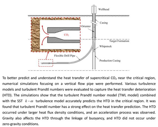
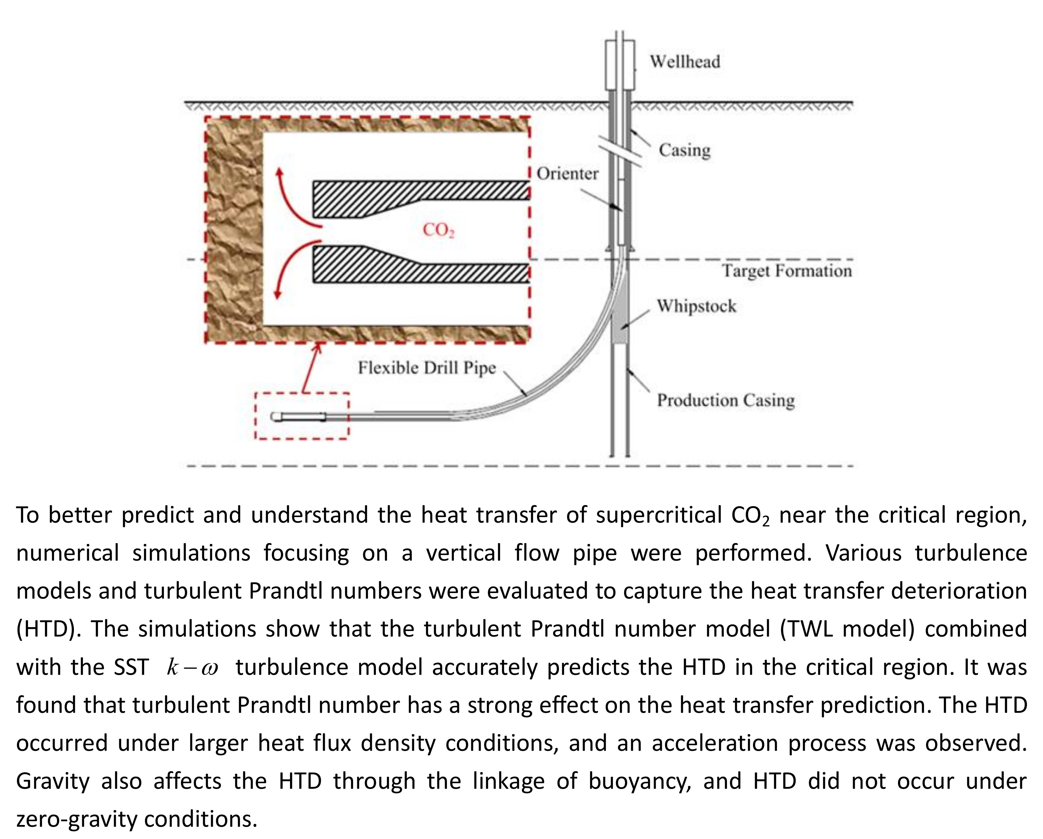
Shale gas is a type of unconventional natural gas that is found trapped within shale formations. In 2000, shale gas only accounted for 1% of U.S. natural gas production, but fifteen years later, it accounted for nearly 50% [1]. The boom of shale gas production is mainly due to the wide use of hydraulic fracturing, a well-stimulation technique in which rock is fractured by a pressurized fluid (primarily water containing sand or other proppants suspended with the aid of thickening agents) [2,3,4]. However, more and more studies have argued that hydraulic fracturing may raise a number of environmental problems: (1) a large amount of water is required for one shale gas well [5]; (2) more than 20 types of additives are added in the injection water, such as hydrochloric or muriatic acid, gelling agents, and chemical modifiers, which may contaminate groundwater [6,7]; (3) large-scale water disposal via deep re-injection has been linked to trigger seismicity that results in low-level earthquakes [8,9,10]; (4) other issues include accidental chemical spills, waste disposal, air pollution, and the land footprint of drilling activities [11]. Economic pressures and environmental targets drive people to use new methods to exploit shale gas. Recently, the use of supercritical carbon dioxide (SC-CO2) instead of water to drilling and fracture shale has been proposed (Figure 1), whereby liquid CO2 from a bulk supply would be pumped through the high-pressure tube using a high pressure plunger pump. The results of experiments have demonstrated that supercritical carbon dioxide (SC-CO2) jets will cut hard shale, marble and granite at much lower pressure than water [12].
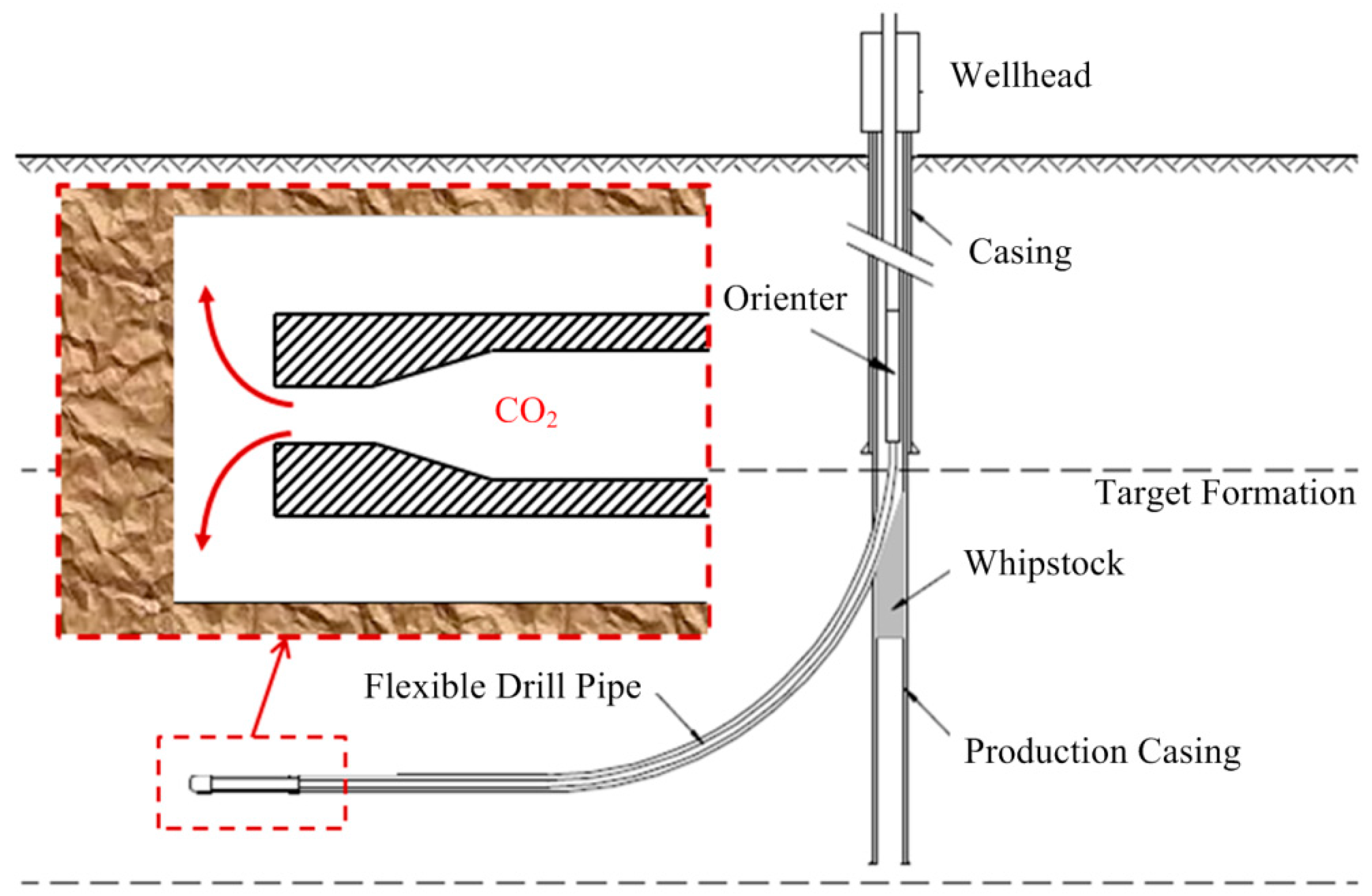
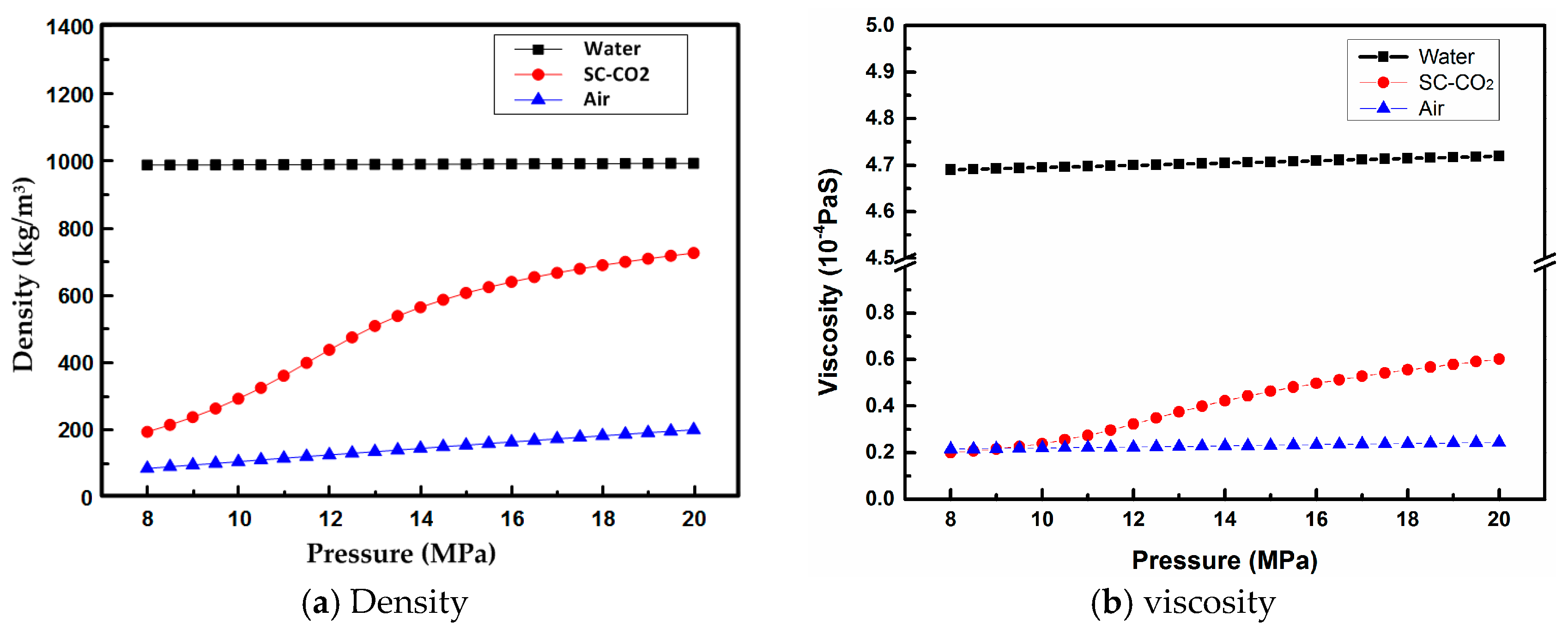
However, different from traditional drilling mud and fracturing fluid, the SC-CO2 play ultimately characteristics in the wellbore due to the variation of carbon dioxide (CO2) properties. The physical properties of carbon dioxide are shown in Figure 2. Like other supercritical fluids, SC-CO2 has the unique properties of a gas-like viscosity and a liquid-like density [13,14]. The high density helps SC-CO2 to break rock like water does, while the low viscosity could decrease the dissipation of energy from the nozzle to the rock [15,16,17]. Additionally, the high diffusivity allows SC-CO2 to enter deep fractures and pores and transmit the fluid static pressure, which is helpful to improve the rock-erosion efficiency [18,19,20]. Middleton et al. [21] outlined the potential advantages of SC-CO2 to exploit shale gas: (1) increased shale gas production through additional fractures and reduced flow blocking and desorption; (2) reduced types and amounts of additives, thereby reducing the contamination to groundwater; and (3) reduced or eliminated water requirements, thereby reducing re-injection and the frequency of low-level earthquakes.
The thermal and cooling pretreatments are required before SC-CO2 is injected into the formation. After the SC-CO2 is injected into the shale formation, a series of heat transfers occur in the rockshaft due to the subterranean heat. The unique physical properties of the SC-CO2 make the heat transfer process very complex, making it necessary to further study the heat transfer of SC-CO2.
In general, there are three different types of heat transfer for supercritical fluids: normal heat transfer, intensified heat transfer and heat transfer crisis. Normal heat transfer [22,23] occurs far from the critical point regions with a predictable heat transfer coefficient. Intensified heat transfer [24] occurs when heat flux is very low, and a local peak value of the heat transfer coefficient exists near the pseudo-critical point. When the heat flux is relatively higher and mass flow rate is relatively smaller, a heat transfer crisis occurs [25,26]. Due to the multi-type of heat transfer for supercritical fluids, many scholars have studied SC-CO2 heat transfer. Wood and Smith [27] found that when the average temperature of CO2 was greater than the pseudo-critical temperature, the CO2 velocity profile in the vertical tube became smooth, and the distribution was in an “M” shape. Shiralkar and Griffith [28] discussed the SC-CO2 heat transfer in a radical tube with diameters of 0.32 mm and 0.64 mm, which led to a twisted temperature curve. Adebiyi and Hall [29] concluded that gravity and buoyancy were closely related to the CO2 heat transfer. Gungor and Winterton [30] determined that when the mass flow rate increased or the experimental pressure decreased, the thermal conductivity of CO2 correspondingly increased. When the average temperature was greater than the pseudo-critical temperature under operating pressure conditions, the thermal conductivity of CO2 decreased. Polyakov [31] reviewed the mathematical model and solution method of heat transfer under supercritical pressure conditions. Liao and Zhao [32] analyzed the effects of diameter on the Nusselt number of heat transfer in laminar flow. Yoon et al. [33] found that under cooling conditions, the heat transfer coefficient reached its maximum and then gradually decreased. A pressure increase caused the maximum of CO2 heat transfer coefficient to decrease. Under all operating conditions, the increase of the mass flow rate also increased the heat transfer coefficient. Kim et al. [34] researched the effects of the cross-sectional shape on the heat transfer of Fi dioxide. Du et al. [35] concluded that turbulent models were closely related to the heat transfer. Yang et al. [36] discussed the effects of an inclined angle on the heat transfer of SC-CO2. The results showed that the heat transfer coefficient in the horizontal tube were greater than the ones in other inclined angles. Peeters et al. [37] concluded that the thermal development length was closely related to the Peclet number, the dimensionless number and the inlet temperature. Some scholar focus on problem of the heat transfer deterioration of supercritical fluid. Koshizuka et al. analyzed deterioration phenomena in heat transfer to supercritical water based on a parabolic solver for steady-state equations in nu-z two dimensions, a k-ε model for turbulence [38]. Grabezhnaya and Kirillov [39] analyzed the relations for technical calculations of the normal heat transfer in a rising water flow under supercritical pressure (SCP) and compared with recent experimental results. Urbano and Nasuti [40] considered the influence of deterioration of forced convection heat transfer for channel flows of supercritical fluids. Wen and Gu [41] investigated the heat transfer deterioration (HTD) in supercritical water flowing through vertical tube by numerical method. The heat transfer crisis in channel was also investigated by other scholar due to looking forward the characteristics of heat transfer [25,26].
Despite such rewarding developments in the heat transfer of SC-CO2, there is still a relevant degree of uncertainty in the prediction stage that arises from the lack of reliable and universal methods to predict the heat transfer deterioration (HTD). In the present work, a validated prediction method has been proposed to facilitate the near critical heat transfer investigation. Matlab (R2017b, The MathWorks Inc., Natick, MA, USA) codes have been programmed to first calculate the properties of carbon dioxide near its critical point. Then, both the prediction abilities of the constant Pr and the variable Prandtl number model with different turbulence models have been evaluated. Based on the simulation results, the gravity and buoyancy effects on the vertical tube heat transfer of carbon dioxide were investigated.
2. Numerical Methods
2.1. Real Gas Model
The simulation results are strongly dependent on the equation of state (EOS), which shows the relationship between the density, the pressure and the temperature. Since the high-pressure liquid and supercritical regions are the main concern of this work, the Span and Wagner (SW) EOS was used because it is considered to be the most accurate EOS for CO2 and is used as a benchmark for other models [42].
The dimensionless form of the Helmholtz energy [43] can be expressed the sum of as two parts: the ideal-gas behavior and the residual fluid behavior:
The ideal-gas behavior part [42] is given as the following formula:
The residual fluid behavior part is given as:
where:
A simplified empirical equation was obtained by optimizing Equation (3):
2.2. Governing Equations
SC-CO2 was treated as a pseudo-fluid in the current mode. The continuity equation, momentum equation and energy equation are as follows:
2.3. Turbulent Model
2.3.1. Standard k-ε Turbulent Model
The standard k-ε turbulent model is given by Launder and Spalding [44], and is widely applied to engineering fields. The turbulent kinetic energy equation and turbulent dissipation rate equation are as follows:
where ,, align these equations.
2.3.2. Realizable k-ε Turbulent Model
The realizable k-ε turbulent model [45] fully considers the effects of rotation and curvature:
where .
2.3.3. SST k-ω Turbulent Model
The SST k-ω turbulent model [46] integrates the advantages of the standard k-ε turbulent model and the standard k-ω turbulent model:
where .
2.4. Variable Turbulent Prandtl Number Model
The reveals the effects of the fluid physical properties on the heat transfer and is defined by:
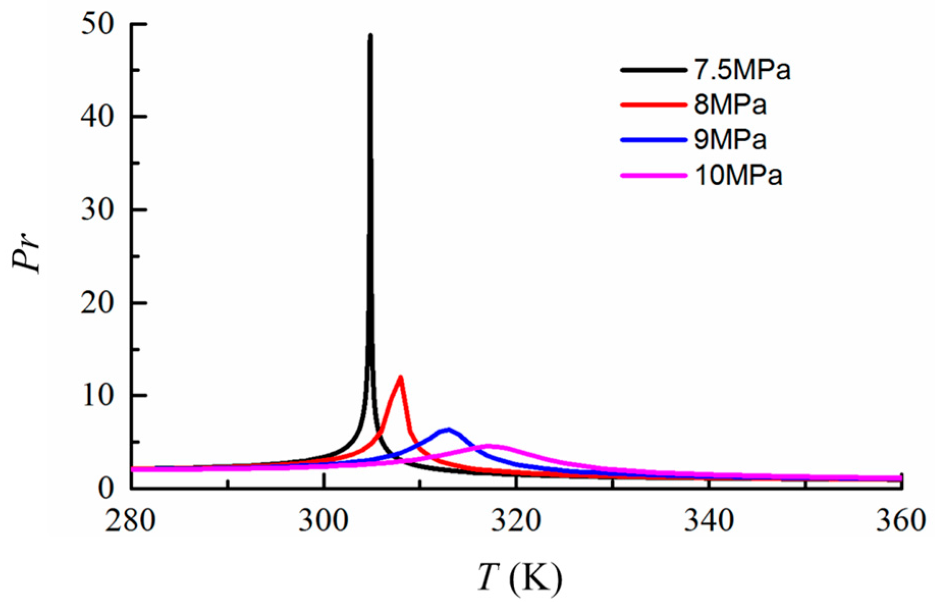
A constant of 0.85 is used, which is the most commonly used value in previous CFD simulations. However, in a supercritical fluid heat transfer, e.g., SC-CO2, experiences large Pr variations in the pseudo critical temperature region (Figure 3). The constant Pr model is questionable to show its rationality in predicting the supercritical fluid heat transfer, especially in HTD cases.
3. Numerical Simulation Setup
3.1. GeometryModel
3.2. Grid Independence Tests
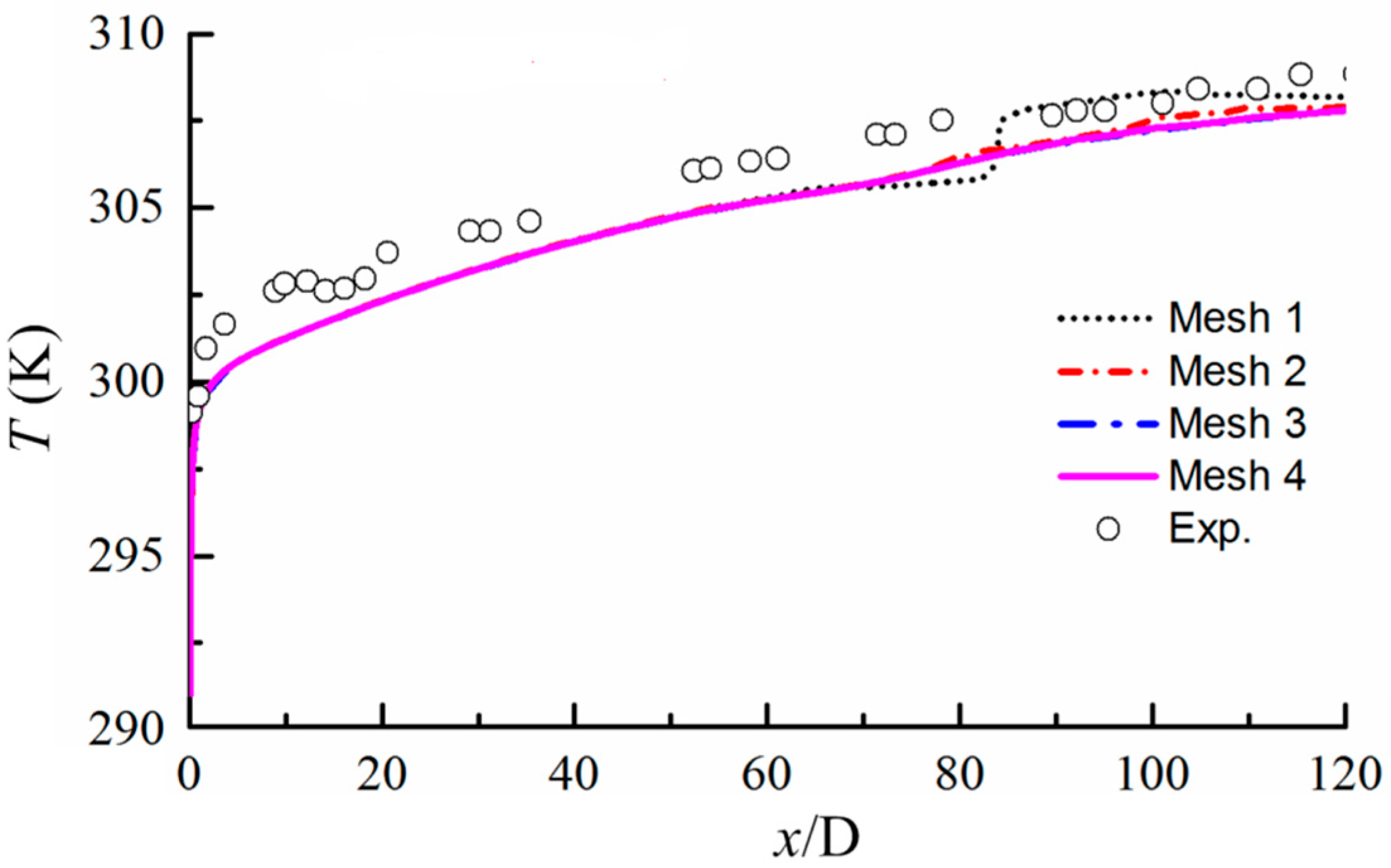
A structured mesh was employed to discretize the computational domain. To verify the independence of the meshes, the wall temperature variation along the axial direction was studied with four different numbers of discrete meshes, as shown in Table 1.
The four different program of structured mesh was compared as following table. Different nodes in the axial and radial direction were distributed in the simulating model. Then the model obtained different number of meshes. The results indicated that when x/D is less than 60, the simulated results of Mesh Program 1 are in good agreement with experimental results. When x/D is greater than 60, for Mesh 1, there is a sudden increase of the tube wall temperature. However, for Mesh Program 2, Mesh Program 3 and Mesh Program 4, the simulated results are in good agreement with experimental results [49], as shown in Figure 5. Thus, a moderate mesh, Mesh 3, was employed to simulate heat transfer in the vertical tube.
3.3. Boundary Conditions
At the inlet, the mass flow rate is 564.32 kg/s, and the outlet was set as the pressure outlet. The boundary conditions were same as the experimental condition conducted [49]. The SIMPLEC algorithm is employed to solve the coupled equations of velocity and pressure, and the QUICK algorithm is employed to solve the energy equation. All residuals are less than 10−5.
4. Results and Discussion
4.1. Model Verification
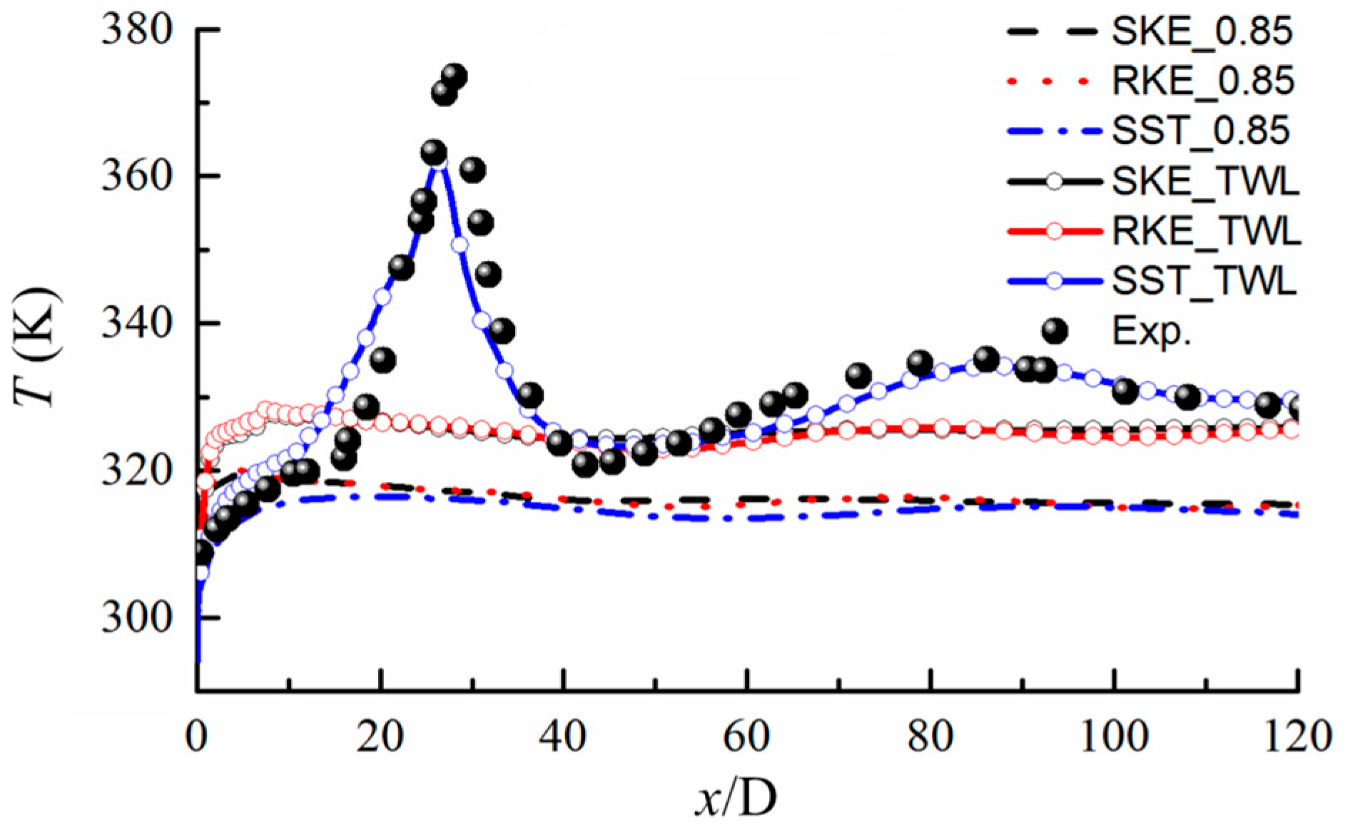
According to the Weinberg’s experimental results, the HTD occured at the heat flux density of 56.7 kW/m2. To select the appropriate model to predict the heat transfer near the critical region, the case with a heat flux density of 56.7 kW/m2 was performed and the comparisons were presented in the Figure 6. It was found that the TWL model with the SST k-ω turbulent model showed greater agreements for the variation tendency of the temperature in the tube wall and the peak value.
4.2. HTD Mechanism and Prt Effects in the Simulation
To deeply understand the effects of the Pr on the prediction of the HTD as well as the HTD mechanism of the supercritical fluid, it is useful to analyze the radial distributions of the predicted key parameters (axial velocity, density, turbulent kinetic energy and turbulent viscosity) in the region near the wall with different Pr models.
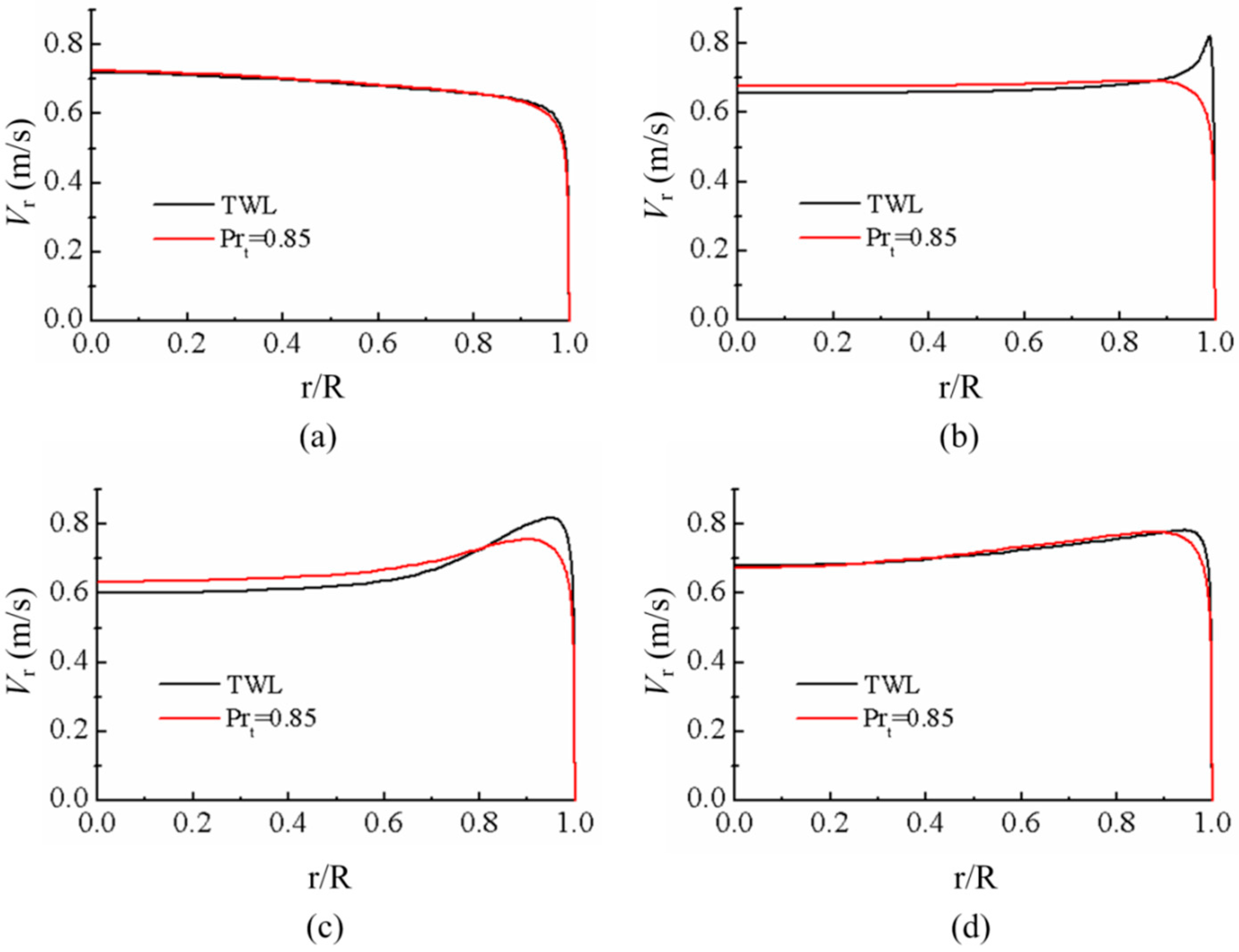
4.2.1. Effects of Pr on the Axial Velocity
When x/D = 13, the distribution of the axial velocity under two different conditions is the same. The section with x/D = 26 is the most intense heat transfer region, and the distribution of the axial velocity has a manifest difference, as shown in Figure 7. In the near wall region, the axial velocity, which is predicted by the TWL model, has one obvious peak. This finding shows that the fluid velocity near the wall increases quickly and then decreases gradually in the radial direction. The distribution appears as an “M”, which coincides with experimental results [27]. The variations of the velocity with Pr = 0.85 does not give an “M” distribution, while the axial velocity with x/D = 39 does. For TWL model, the acceleration process near the wall is more intense, and the prediction value near the axis is less than with the constant model (Prt = 0.85). When x/D = 79, the numerical results of the two models are much closer, and the acceleration process of the axial velocity predicted by the TWL model is more intense.
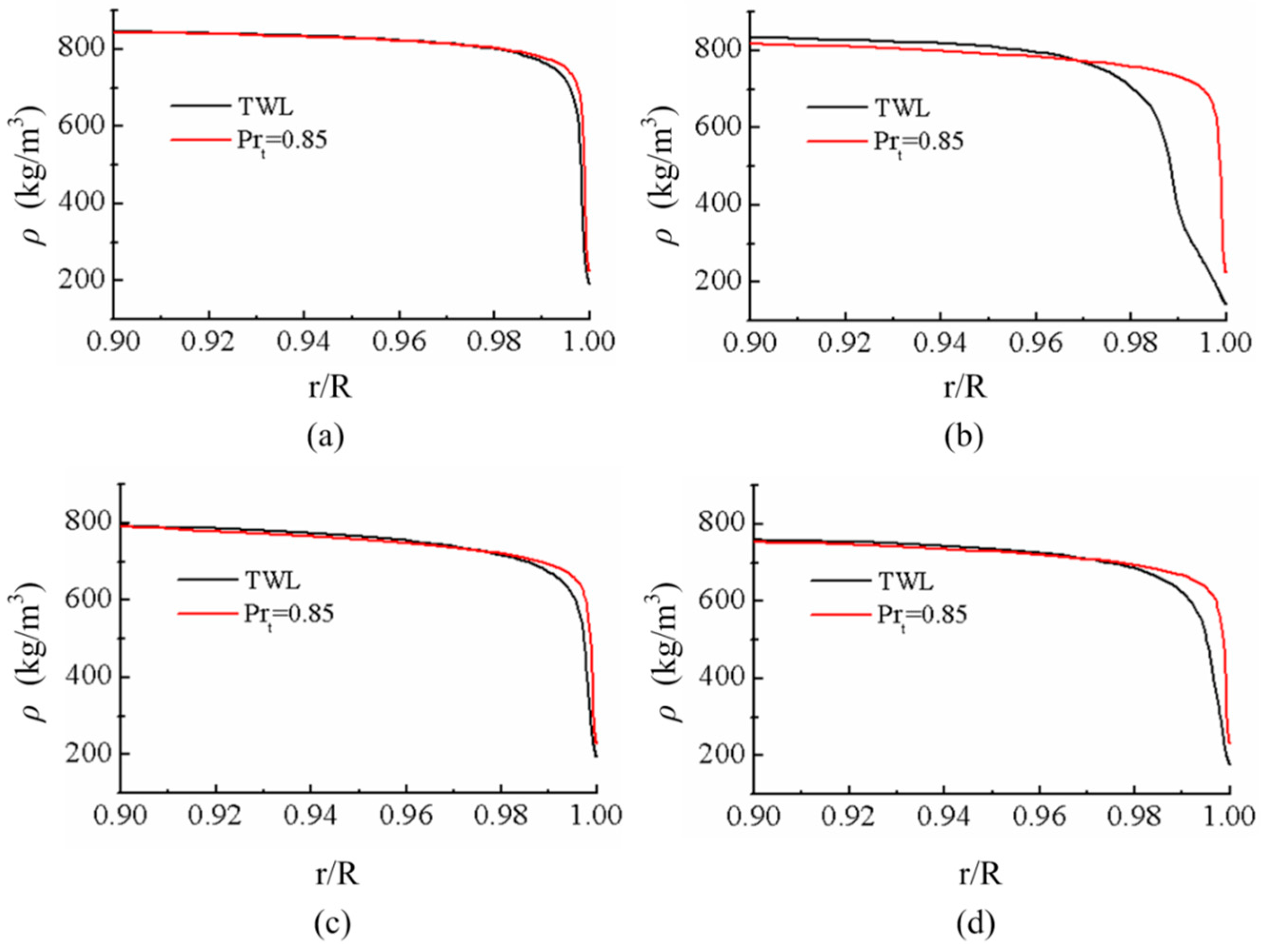
4.2.2. Effects of Pr on the Density
As shown in Figure 8, when x/D = 13, 39 and 79, variations of the density in the region far from the wall are identical. Numerical results of the TWL model are less than the constant model (Prt = 0.85) in the near wall region because the density decreases as the temperature increases. This finding shows that the numerical results of temperature are higher than the constant model. In the most serious heat transfer crisis region (x/D = 26), the numerical results of the two different models has obvious differences. For the TWL model, variations in the density in the near wall region are twisted, which coincides with experimental results given by Shiralkar et al. [45]. For the constant model, the results are similar with other sections. In the heat transfer crisis region (x/D = 79) for the TWL model, the density variation rate is smoother than in the constant model, which indicates the temperature gradient is lower than in the constant model.
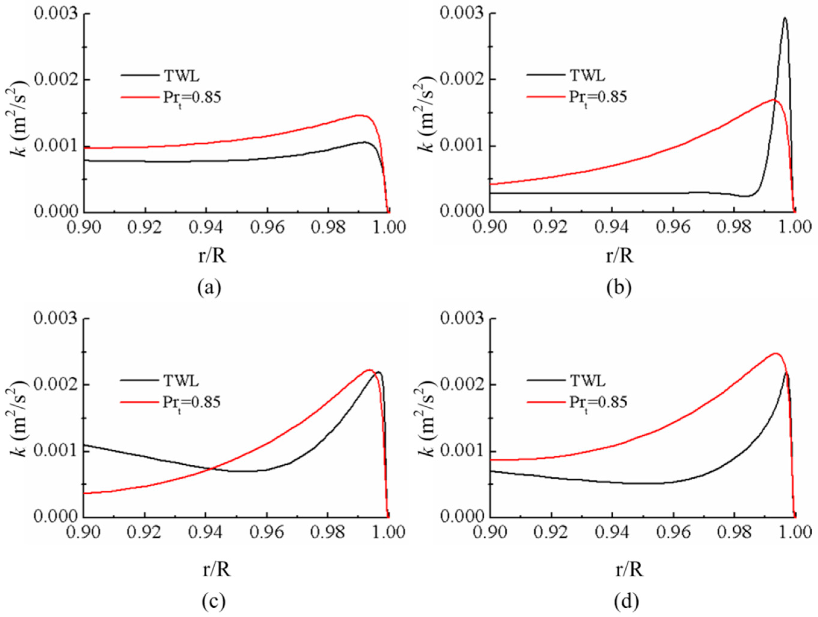
4.2.3. Effects of Pr on the Turbulent Kinetic Energy
In the heat transfer crisis region, one larger turbulent kinetic energy peak value calculated by the TWL model exists in the near wall region, which decreases quickly in axial direction. See the Figure 9, this finding shows that in the heat transfer crisis region, the turbulence converts into laminar flow, which is a key cause of the heat transfer crisis. For the constant model, the turbulent kinetic energy in different sections is identical, and the values in the normal heat transfer region are larger than in the TWL model.
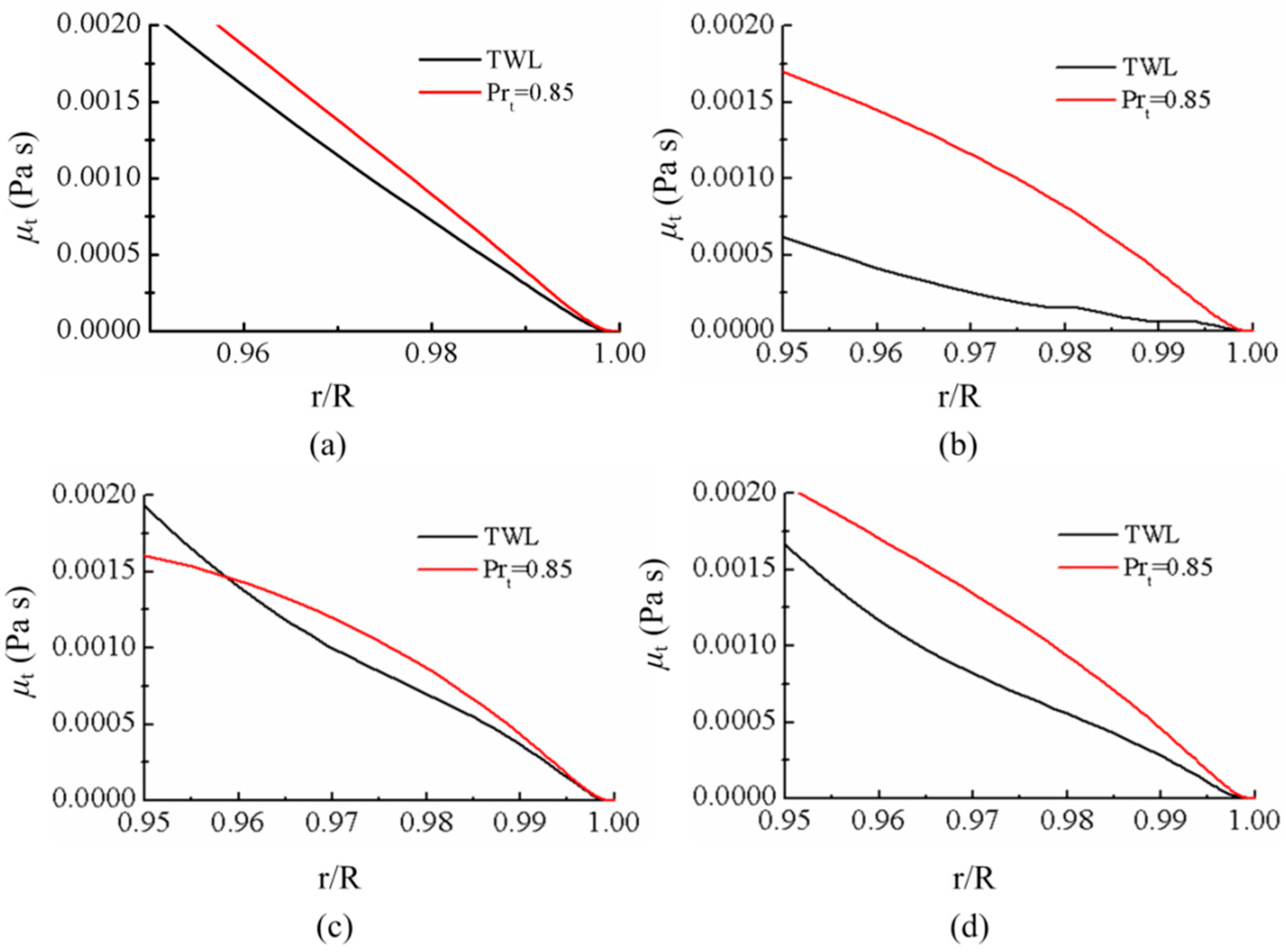
4.2.4. Effects of the Pr on the Turbulent Viscosity
In a given section, the turbulent viscosity grows gradually with the increase in the wall distance. For the TWL model, the numerical results in the region near the wall are lower than in the constant model. In heat transfer crisis region, the difference in the numerical results is manifest. When x/D = 26 (see Figure 10b), the predicted value from the TWL model is lower than in the constant model. The decrease in the turbulent viscosity decreases both the turbulent mixing and heat transfer of the fluid, which allows the local wall temperature to increase, causing the heat transfer crisis. In the given pressure, with the increasing temperature, the carbon dioxide viscosity and turbulent viscosity ratio decrease, as shown in Figure 10. In the heat transfer crisis region, the numerical results of the TWL model are much lower than in the constant model.
4.3. Effects of Heat Flux on Heat Transfer
Based on the SST k-ω turbulent model with the TWL model, the heat flux density is changed to determine its effect on the heat transfer. In the experiment, the inlet mass flow rate is 564.32 kg/m2s, the temperature is 287.15 K, and the pressure is 7.58 MPa. The heat flux densities are 10.1 kW/m2, 30.9 kW/m2, 40.5 kW/m2, 51.9 kW/m2 and 56.7 kW/m2. The heat transfer crisis and heat transfer enhancement are closely related to the heat flux and mass flow rate. Therefore, the q/G is employed to research the effects of heat flux on the heat transfer.
4.3.1. HTD Identification
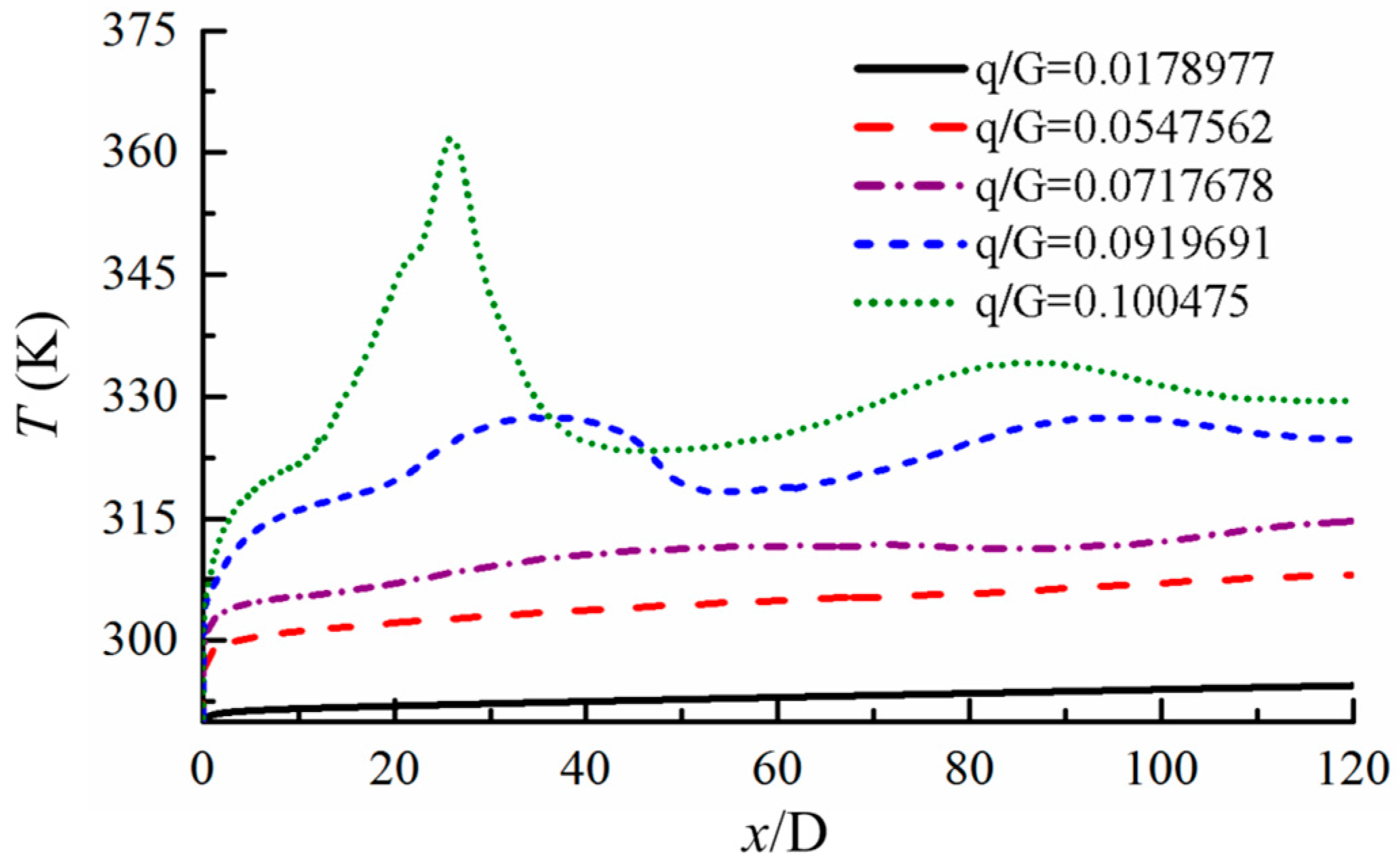
With the increasing heat flux, the heat transfer of the supercritical carbon dioxide shows the obvious variation law (Figure 11). When q is relatively much smaller, the pseudo-critical temperature does not appear. In the axial direction, the wall temperature increases smoothly. As q increases, the increase of tube wall temperature at the inlet tube is more obvious. Then, the distribution of the tube wall temperature is parallel to the smaller heat flux condition, such as q/G = 0.0178977 and q/G = 0.0547562. As q increases further, the temperature does not increase linearly. When q/G = 0.0919691, one local peak value appears and the heat transfer crisis occurs. When q/G is greater than 0.1, the local peak value is much larger, and the heat transfer crisis region is much closer to the inlet of tube. The local peak value moves forward as q increases. Therefore, q has a substantial influence on the heat transfer law of SC-CO2. When the pressure and inlet temperature are constant, an increase in q could weaken the heat transfer to cause a crisis. When this happens, the local wall temperature peak value increases as q increases and appears ahead of the crisis.
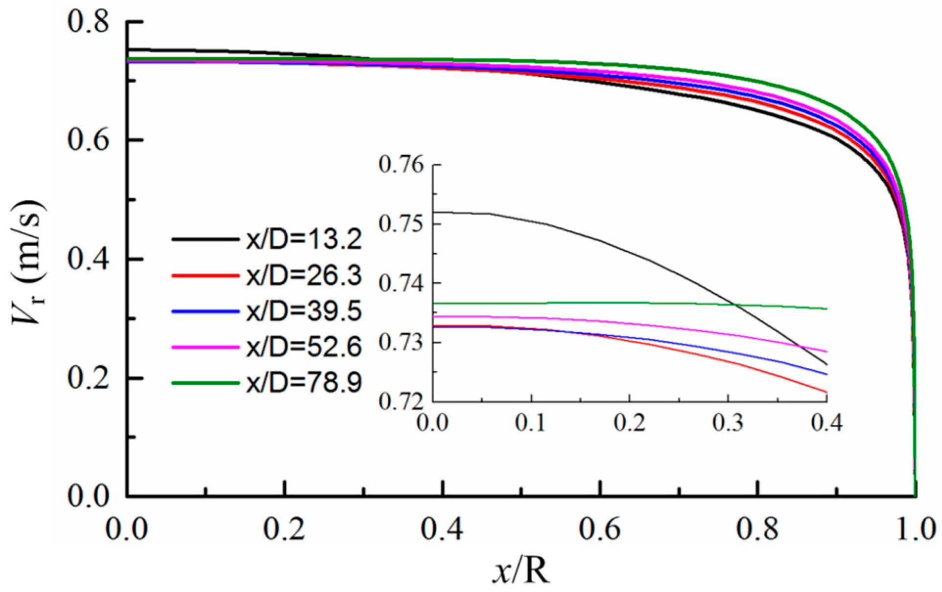
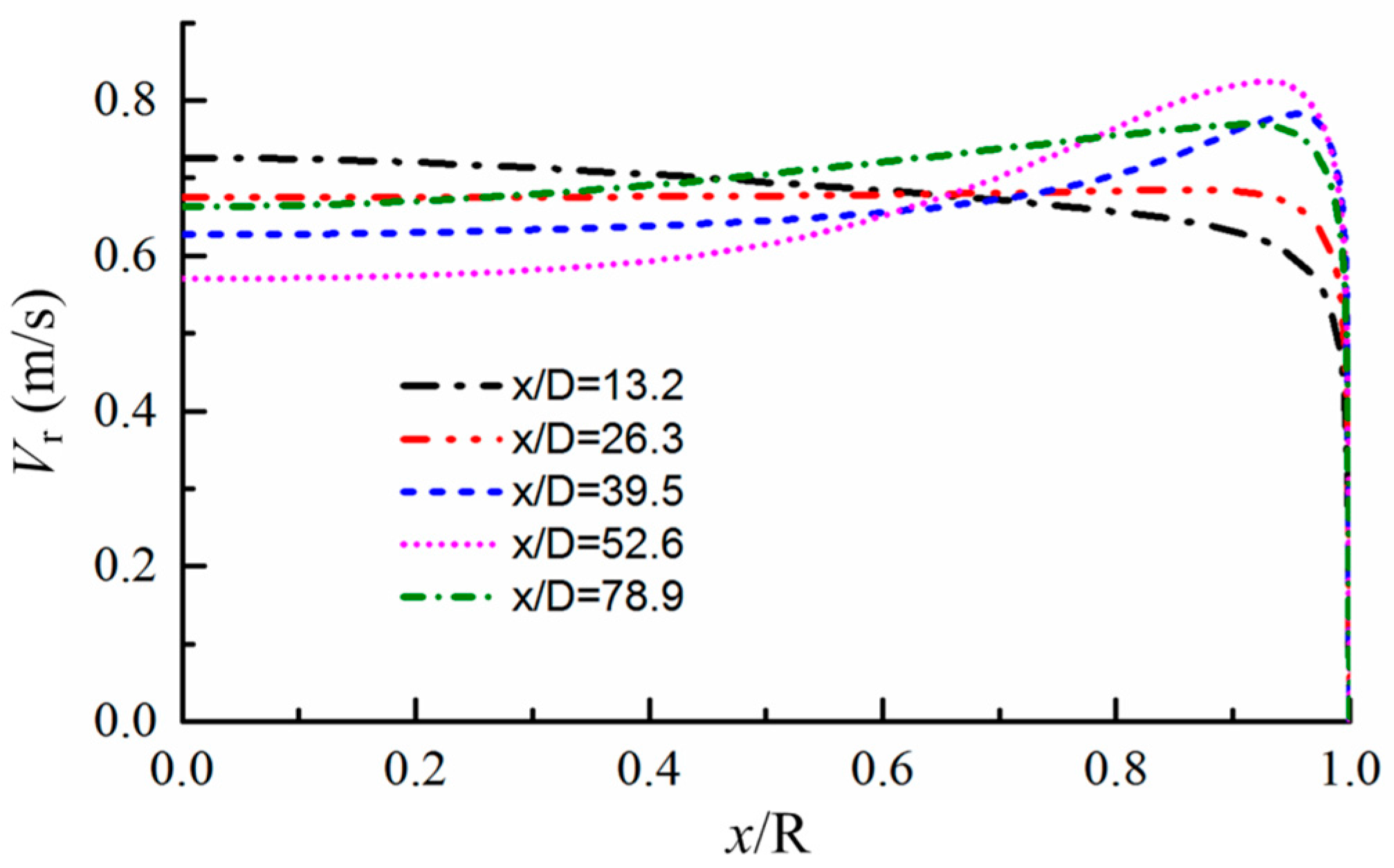
Figure 12 shows the distribution of the axial velocity under smaller heat flux densities over one normal heat transfer period. The velocity distribution far from the wall region is smooth. When x/D = 78.9, the velocity in the center of the tube is constant. Figure 13 gives the distribution of the axial velocity the when heat transfer crisis happens. Before it happens, the velocity distribution appears as a “hat”, and when the crisis occurs, the distribution changes to an “M”.
4.3.2. Effects of Heat Flux on HTD
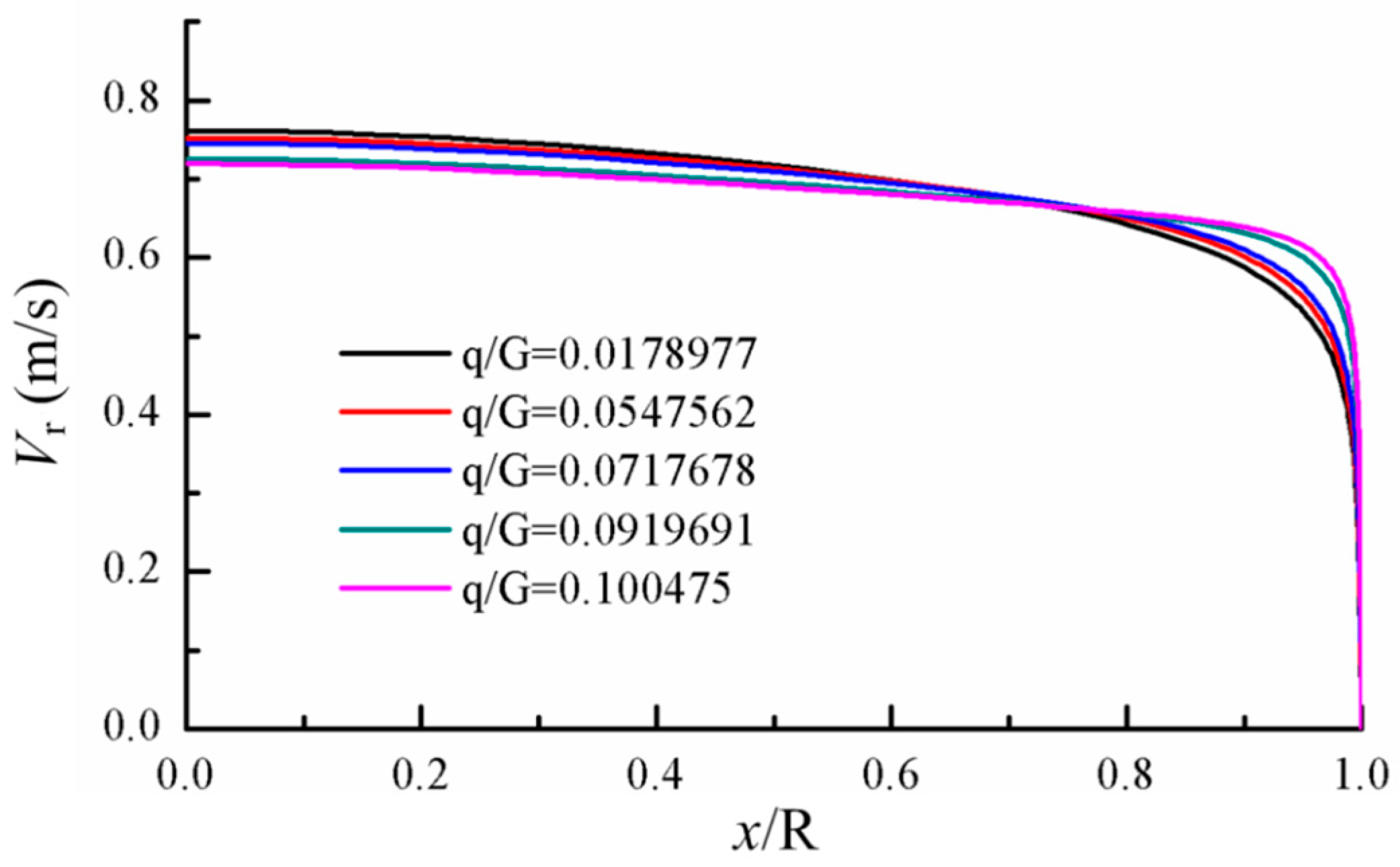
Distributions of the axial velocity, turbulent kinetic energy and turbulent viscosity with x/D = 13.2 are shown in Figure 14, Figure 15 and Figure 16, respectively. In this section, heat transfer does not occur. Therefore, the distribution of the axial velocity, turbulent kinetic energy and turbulent viscosity with different q values have the same variation trend. As q grows, the turbulent kinetic energy and turbulent viscosity near the wall gradually decrease. The distribution of the axial velocity in the radial direction is a typical velocity distribution of forced convection tubes. Near the wall, the velocity gradient is very large, and in the main flow area, distribution of velocity is smooth.
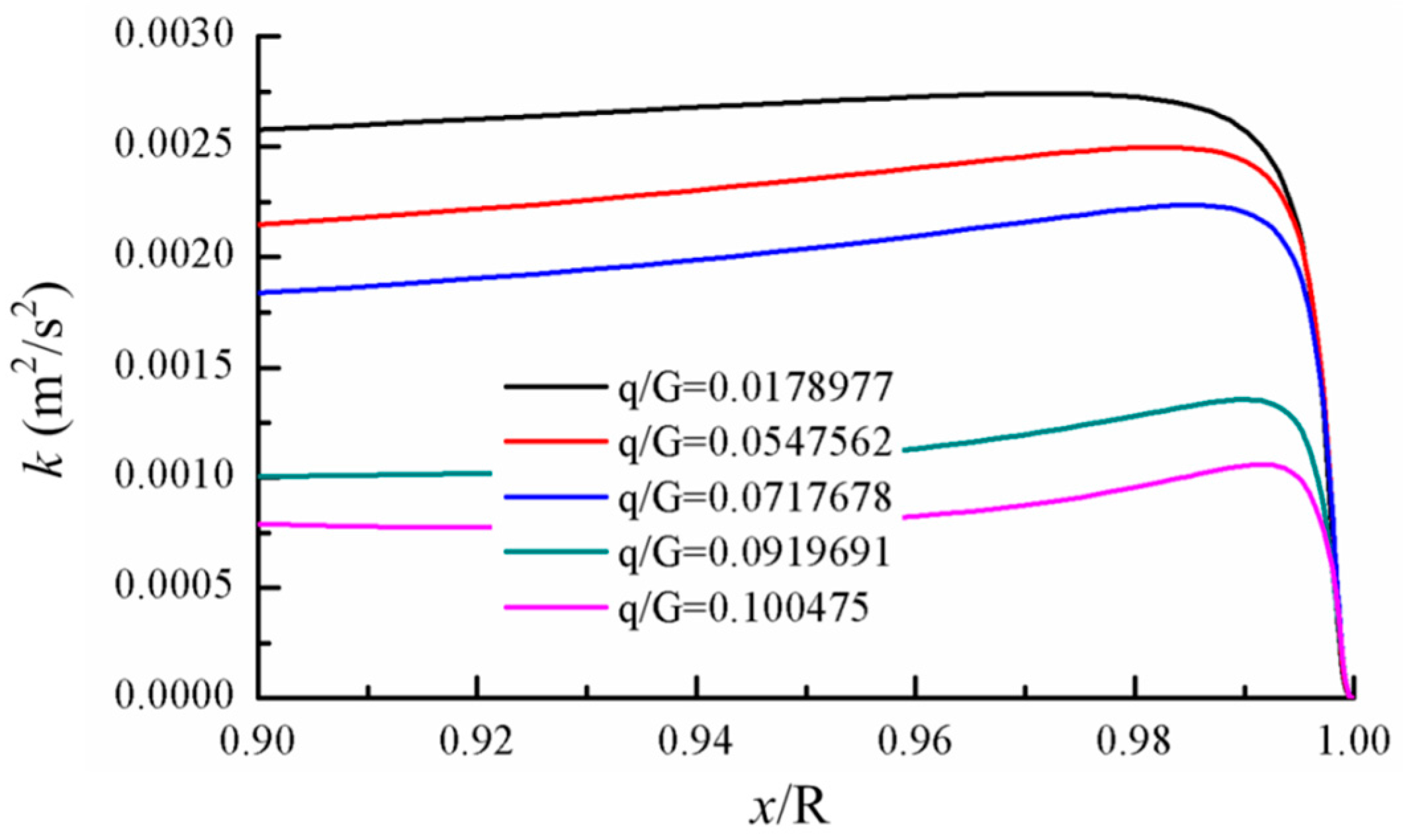
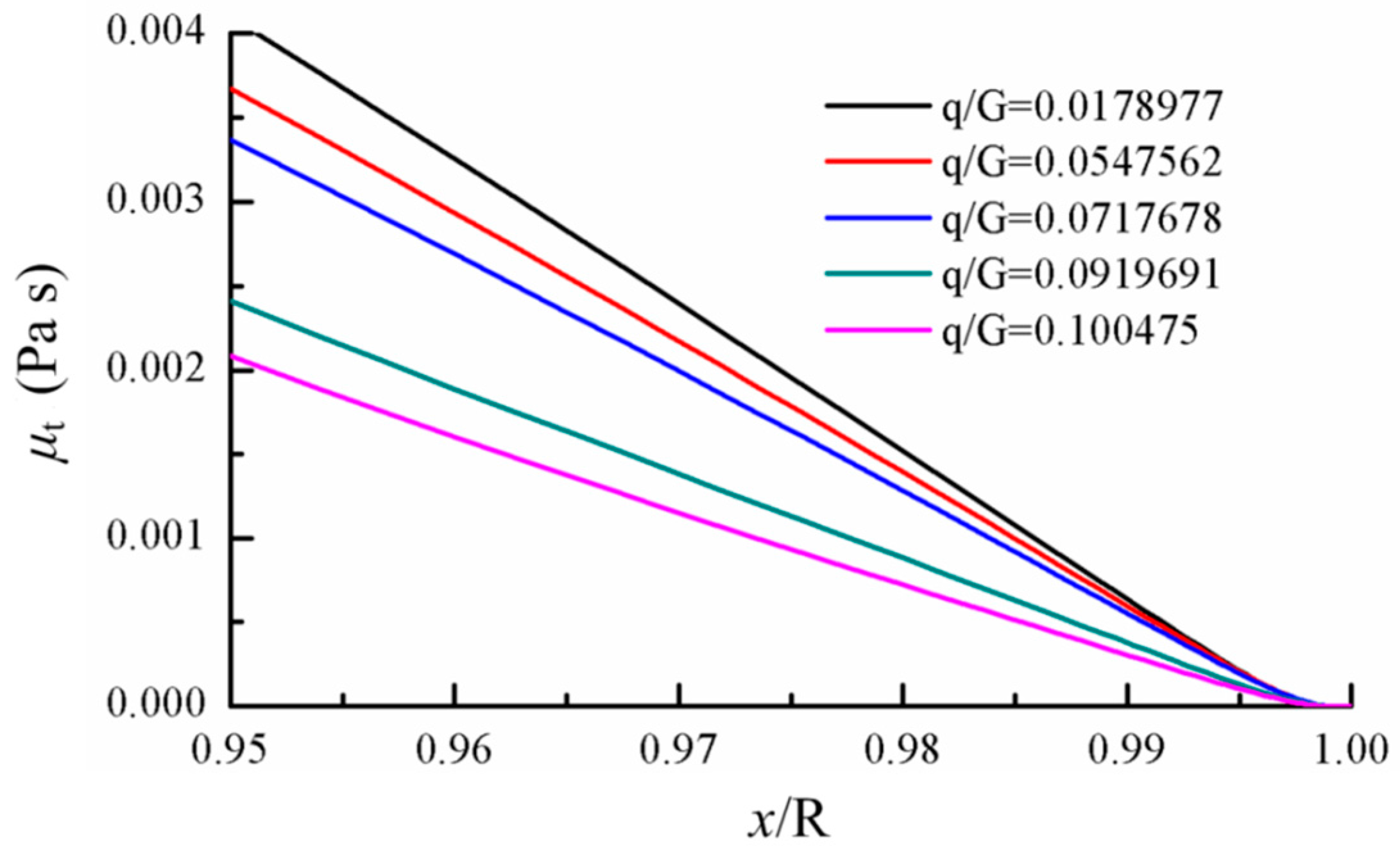
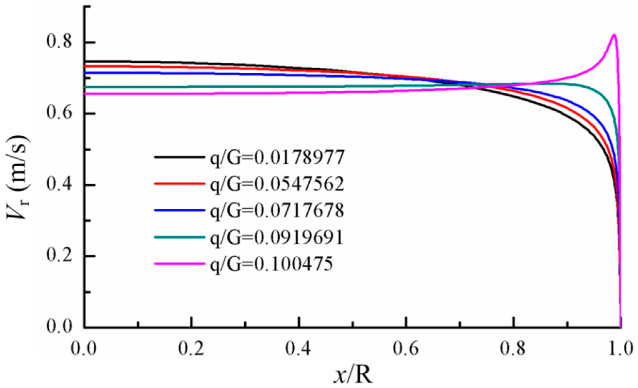
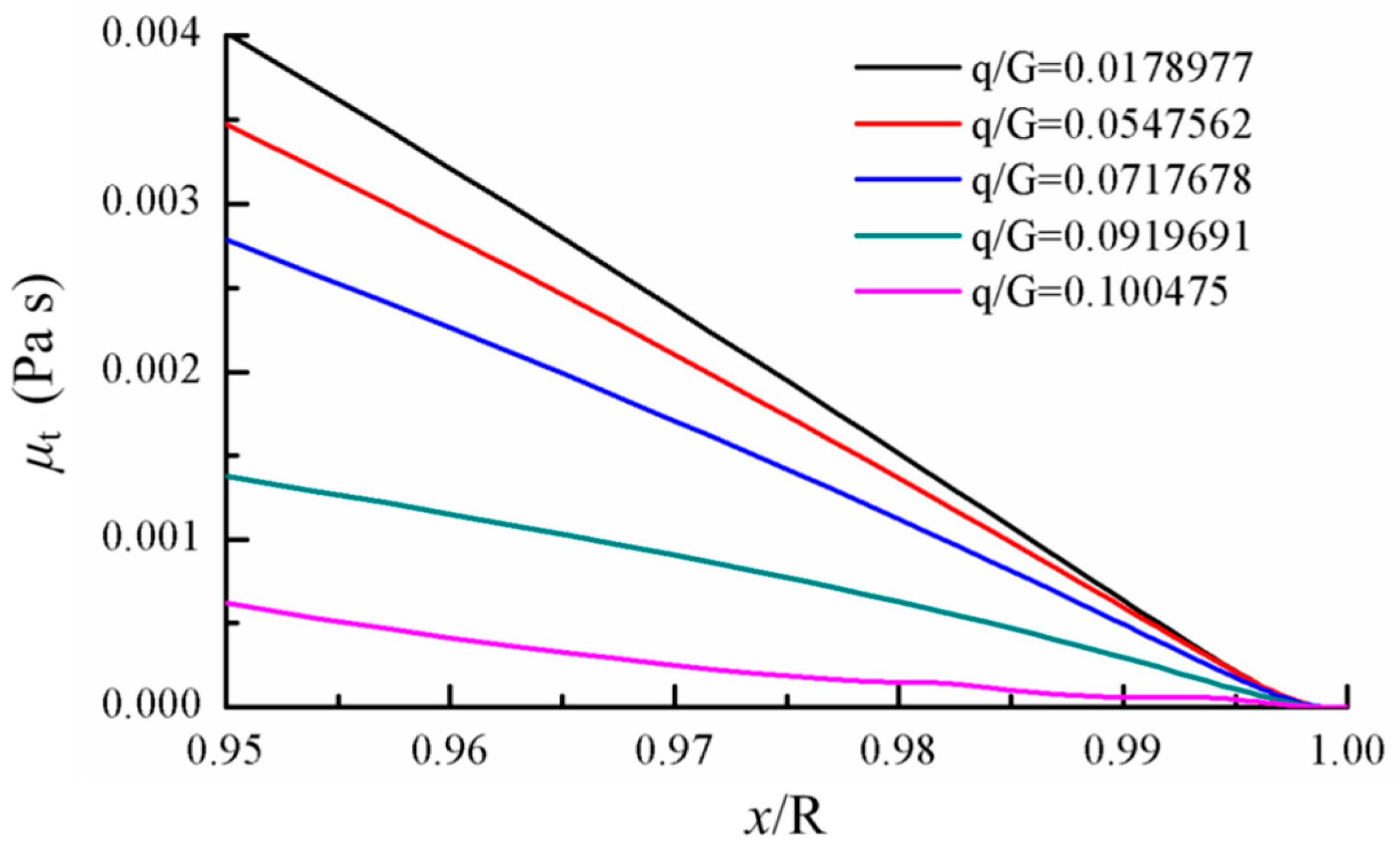
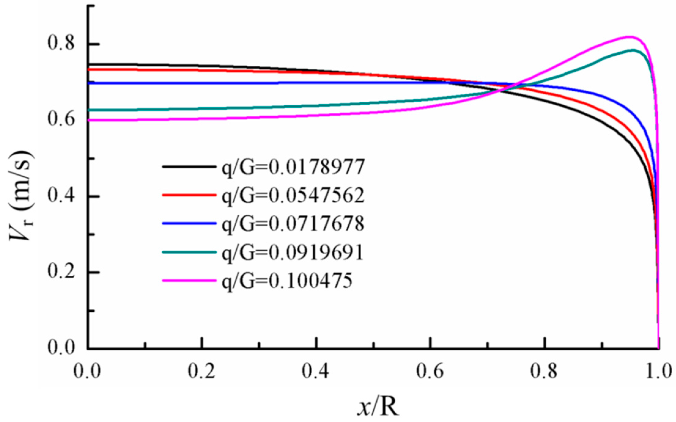
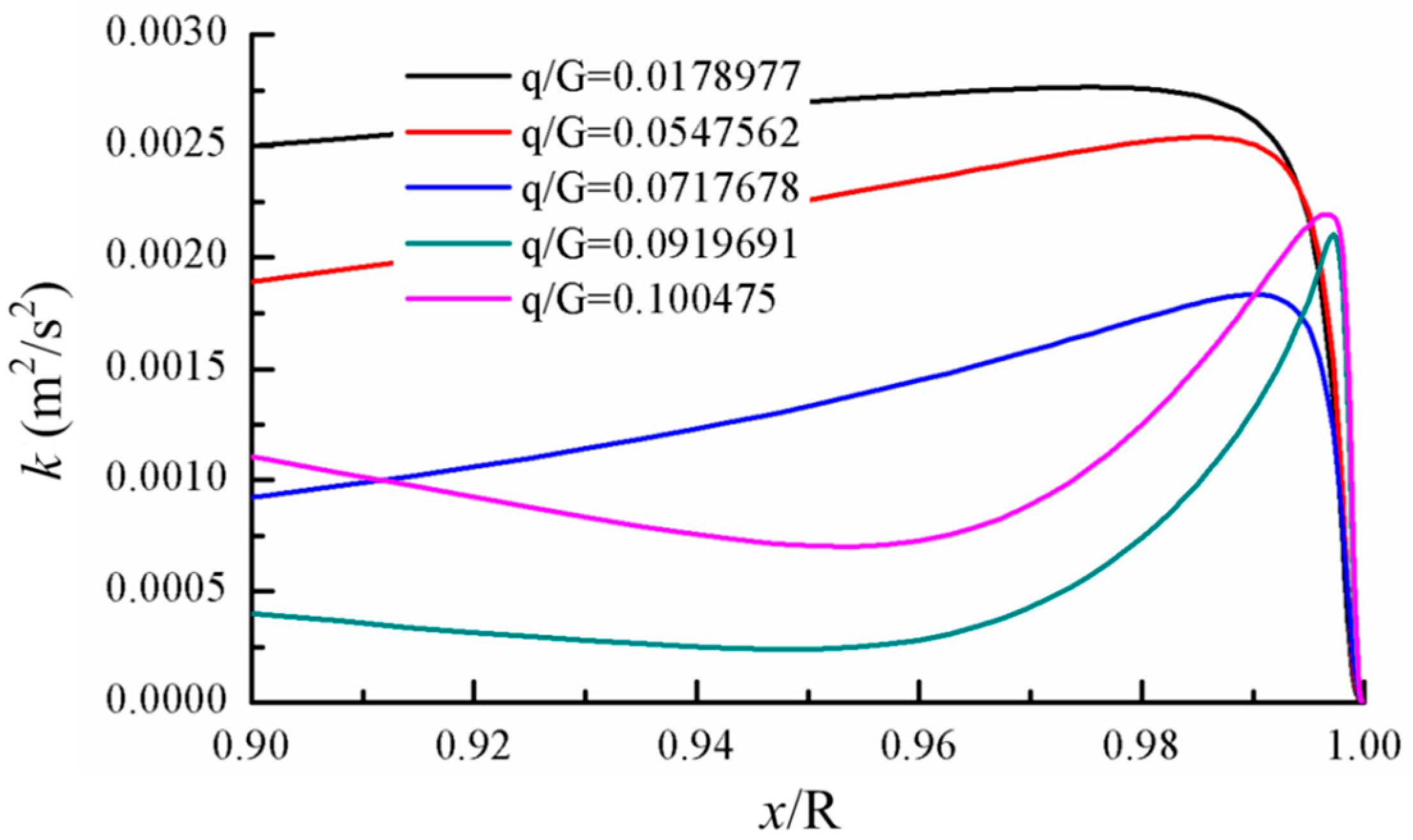
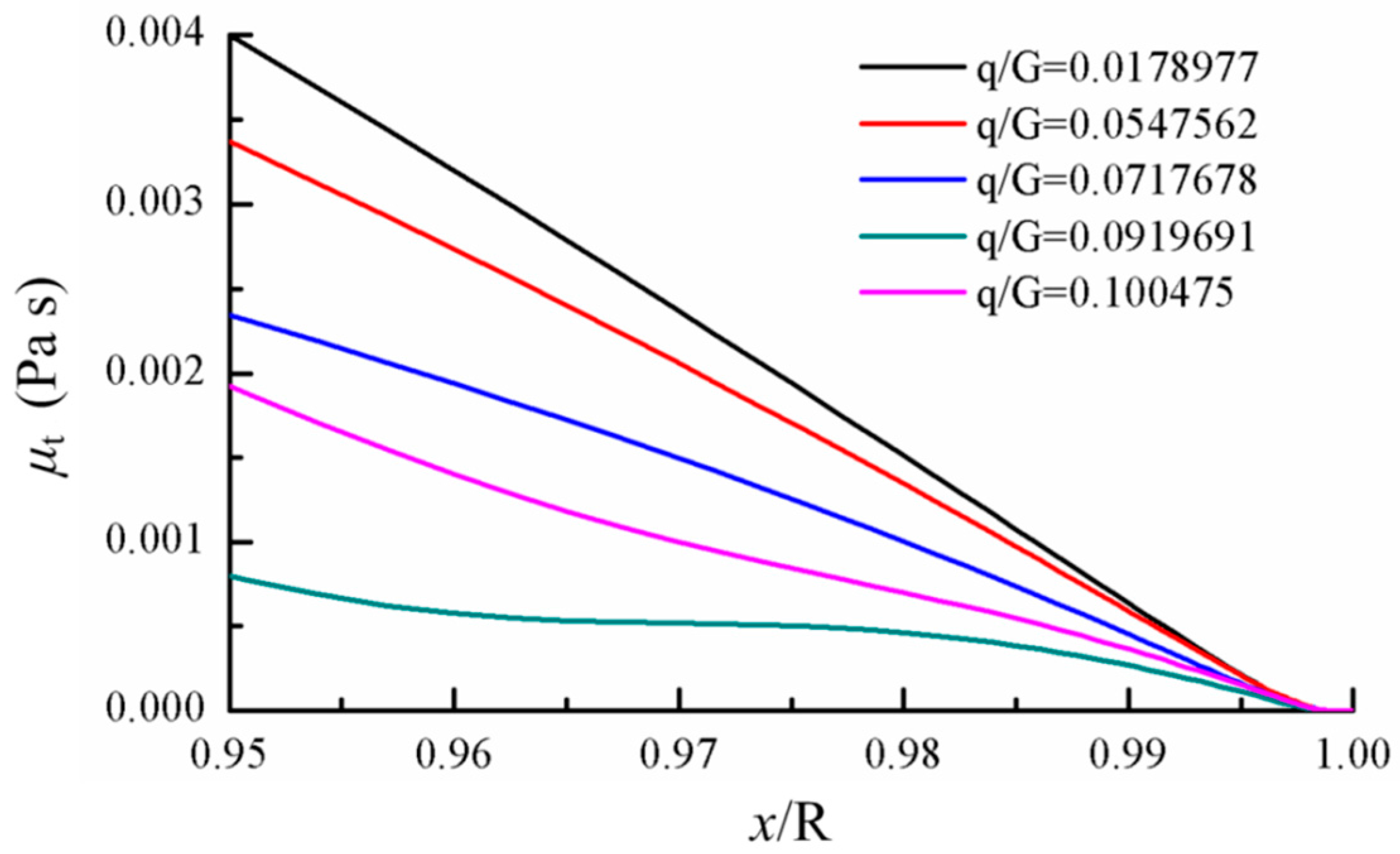
When x/D = 26.3, the local temperature peak value appears when q/G = 0.100475 and when heat transfer occurs. In this case, the axial velocity gradient near the wall is maximized and a greater peak value exists (Figure 17). In the main flow region, the velocity gradually decreases. The distribution of the axial velocity under smaller heat flux densities has the same variation tendency. In this section, the turbulent kinetic energy near the wall when q/G = 0.10047 grows rapidly to its maximum and then decreases rapidly (Figure 18). However, the turbulent kinetic energy in the other conditions does not have this distribution. The distribution of the turbulent viscosity has a similar tendency. As shown in Figure 19, under the heat transfer crisis conditions, the turbulent viscosity significantly decreases. Under normal heat transfer conditions, the distribution of the turbulent viscosity is similar with the section x/D = 13.2.
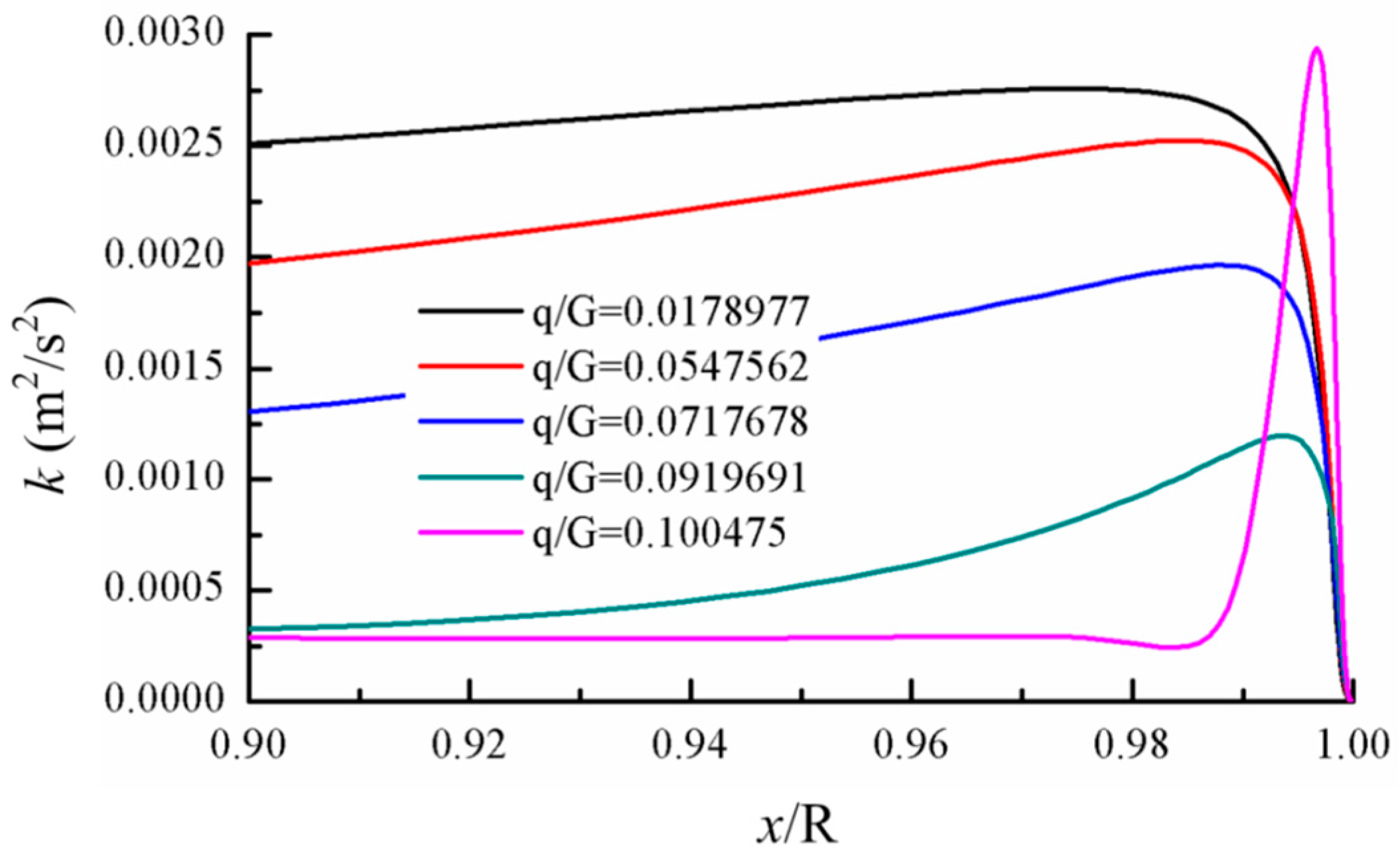
Figure 20 indicated that the distribution of the axial velocity in the section with x/D = 39.5 appears as an “M” due to the effects of heat transfer when q/G = 0.0919691. However, the turbulent kinetic energy near the wall increases rapidly, and then decreases, while the turbulent viscosity significantly decreases (Figure 21). When q/G = 0.091969, heat transfer occurs, but the crisis is weakened, the wall temperature decreases from its peak value to the normal value, and the velocity peak value in the wall decreases. Variation of the turbulent kinetic energy near the wall is smooth, and the turbulent viscosity increases again (Figure 22).
4.4. Effects of Gravity on Heat Transfer Near the Critical Point
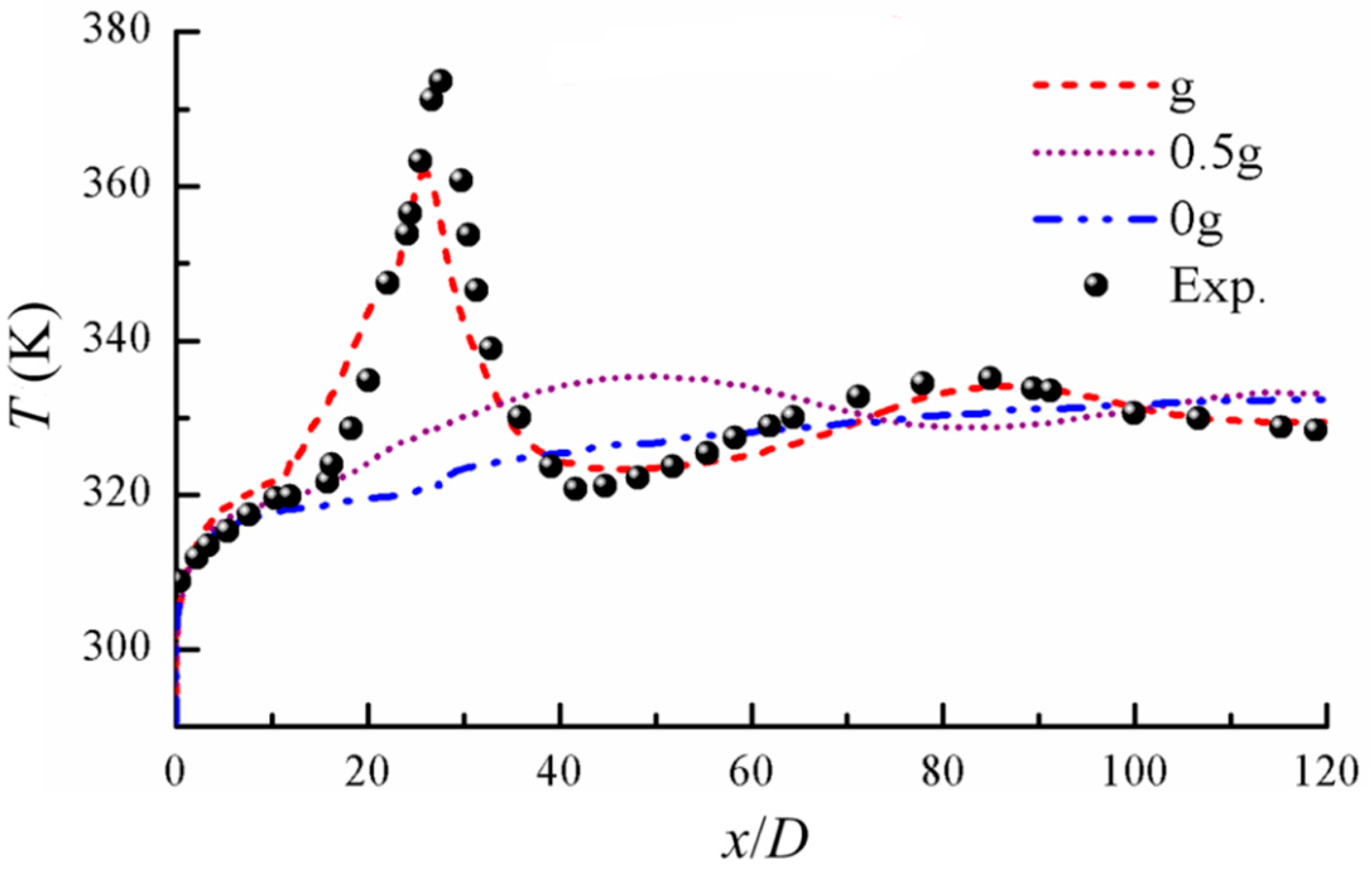
The gravity is changed to explore its effects on the heat transfer near the critical point. As shown in Figure 23, in the experiment, the heat flux density is 56.7 kW/m2, the inlet mass flow rate is 564.32 kg/m2·s and the inlet temperature is 287.15 K. The gravity values include full gravity (1.0 g), half gravity (0.5 g) and zero gravity (0.0 g). Under full gravity conditions, the numerical results are in good agreement with the experimental results. Under half gravity conditions, the local wall temperature peak value decreases dramatically and moves towards the downstream of the vertical tube. Under zero gravity conditions, an obvious local wall temperature peak value does not exist. At the inlet, the wall temperature rises quickly. When x/D is greater than 10 D, the temperature rises smoothly as the heating distance increases. Therefore, under this condition, gravity has a considerable influence on the numerical results. The buoyancy caused by gravity has a close relation with the heat transfer, which is in accordance with theoretical results [50].
4.4.1. Effects of Gravity on the Axial Velocity
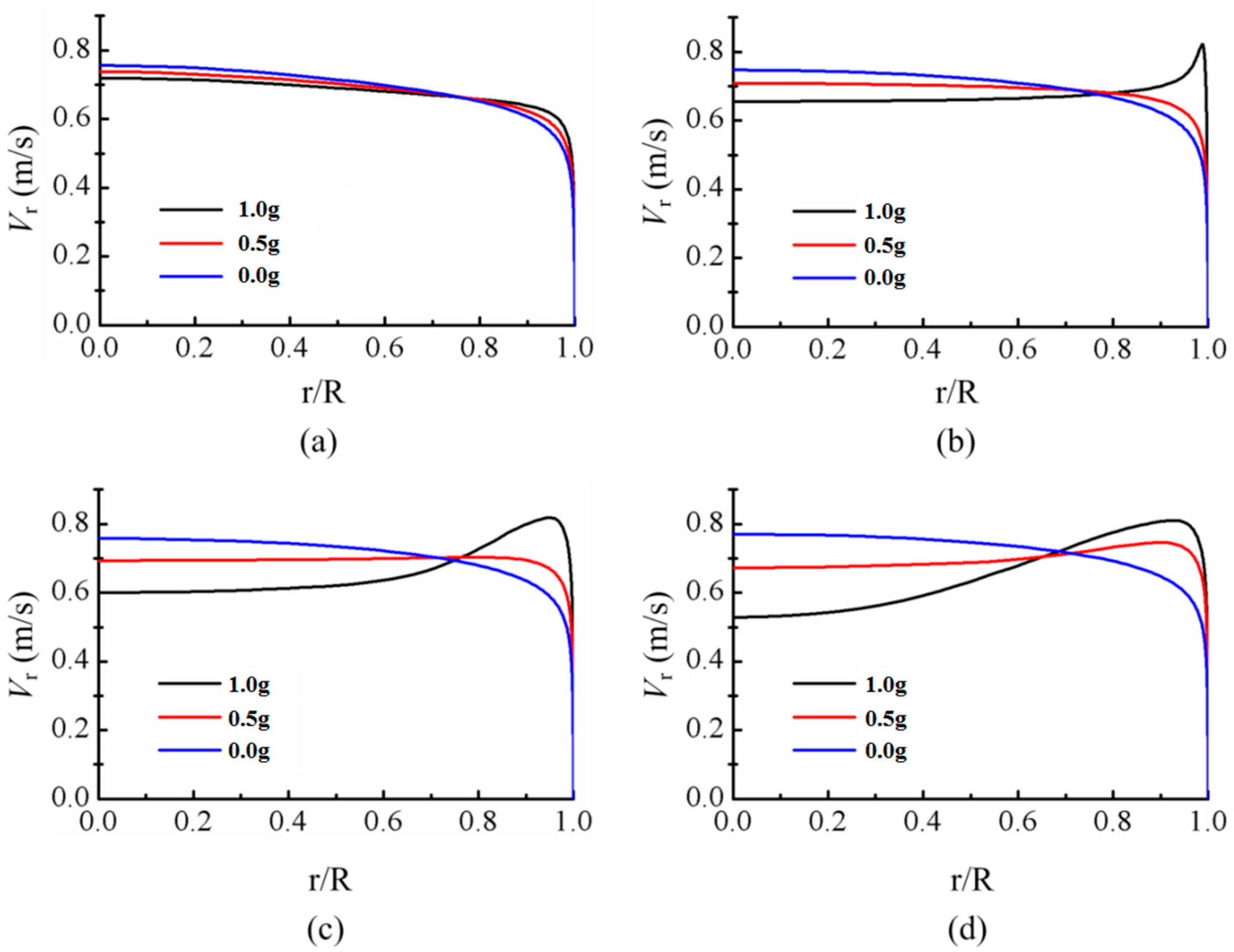
Compared the results of axial velocity and analyzed the influence of gravity from Figure 24. When x/D = 13 (Figure 24a), under the three different gravity conditions, the distribution of the axial velocity is identical to the full development velocity in the tube. In the section with x/D = 26 and under full gravity conditions (Figure 24b), fluid near the wall accelerates locally. As gravity grows, the velocity distribution in the center of the tube is smooth with a gradually decreasing value. In the section with x/D = 39 and under zero gravity conditions (Figure 24c), the velocity distribution remains unchanged. Under half gravity conditions, the velocity in the center of tube is constant. Under full gravity conditions, the local velocity peak value near the wall begins to decrease. In the section with x/D = 53 and under half zero gravity and full gravity conditions (See Figure 24d), the maximum velocity exists near the wall, and the distribution appears as an “M”. Therefore, the buoyancy, which is caused by gravity, influences the velocity distribution to change the heat transfer of supercritical carbon dioxide.
4.4.2. Effects of Gravity on the Turbulent Kinetic Energy
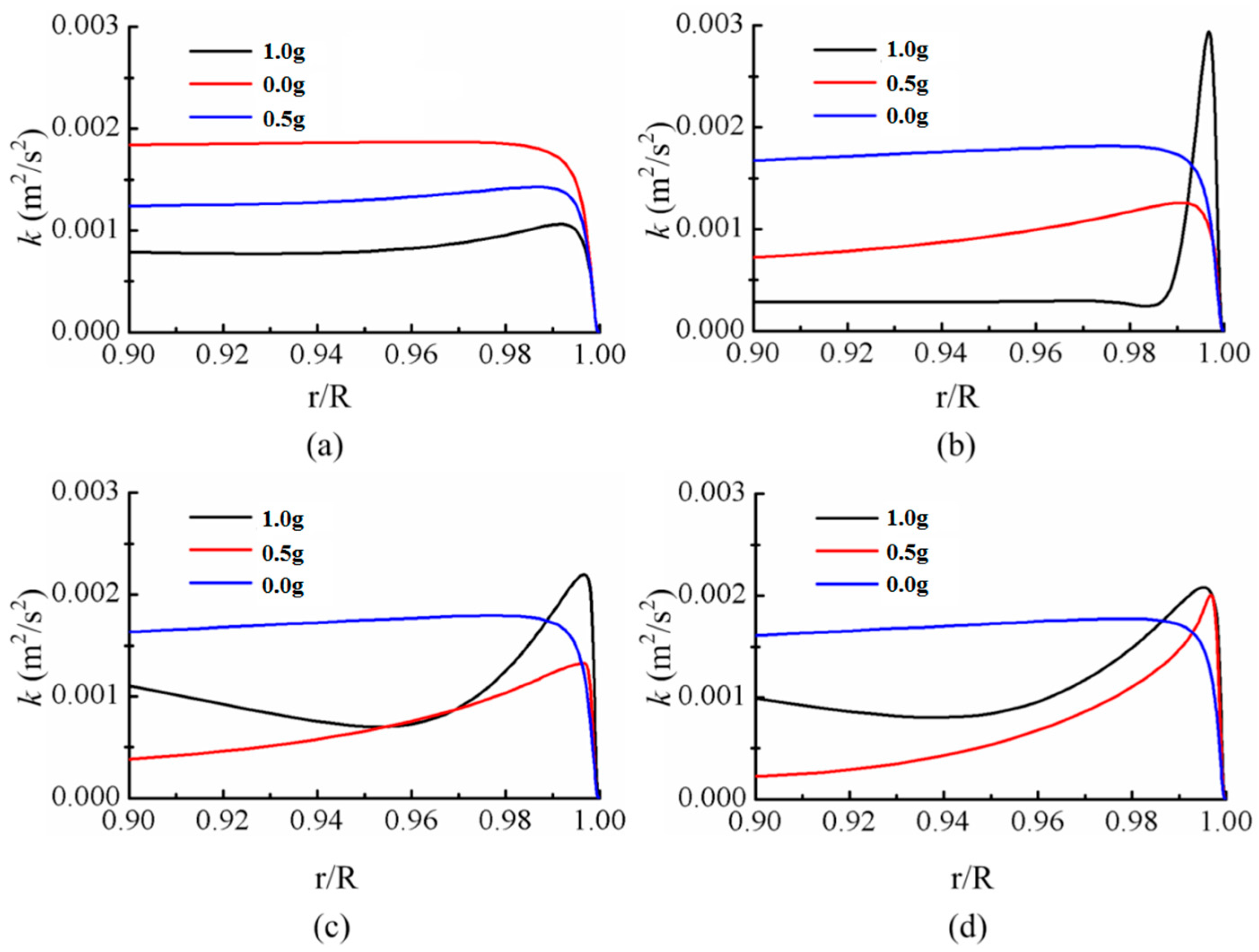
Compared the results of turbulent kinetic energy and analyzed the influence of gravity from Figure 25. When x/D = 13 (Figure 25a), the distribution of the turbulent kinetic energy near the wall is constant. From zero gravity to full gravity, the turbulent kinetic energy near the wall gradually deceases. In the section with x/D = 26 and under full gravity conditions (See Figure 25b), the turbulent kinetic energy of the sub layer near the wall increases first and then decreases, and an obvious local peak value forms. The velocity distribution in the regions near the wall is smooth. However, the velocity under half gravity and zero gravity conditions does not have these characteristics. When x/D = 39 and under full gravity and half gravity conditions (See Figure 25c), the local peak value appears in the sub layer near the wall, and the value in full gravity conditions is much larger. For zero gravity conditions, the distribution of the turbulent kinetic energy remains unchanged. In the section with x/D = 53 and under half gravity conditions (See Figure 25d), the local peak value in the sub layer is more obvious, which has the same law of turbulent kinetic energy in the section with x/D = 23.
4.4.3. Effects of Gravity on the Turbulent Viscosity
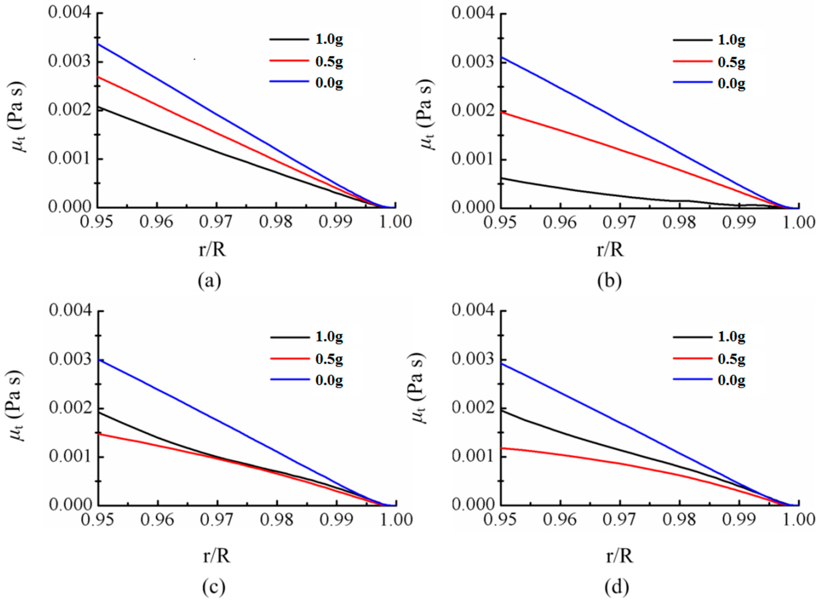
Under different gravity conditions, the turbulent viscosity near the wall has a manifest difference. In the section with x/D = 13 (Figure 26a), the turbulent viscosity near the wall decreases gradually with the increase of gravity. In section with x/D = 26 and under full gravity conditions (Figure 26b), the turbulent viscosity decreases significantly and the flow tends to convert into laminar. Under half gravity and zero gravity conditions, the distribution remains unchanged. In section with x/D = 39 and under full gravity conditions (Figure 26c), the wall temperature and turbulent viscosity become normal, and under half gravity conditions, the wall temperature increases relatively quickly. As a result, the turbulent viscosity decreases. In the section with x/D = 53 and under half gravity conditions (Figure 26c), the wall temperature local peak value appears and the turbulent viscosity is minimized. The flow tends to become laminar and the local heat transfer crisis appears. For the four different sections under zero gravity conditions, the turbulent viscosity near the wall remains unchanged and local heat transfer crisis does not appear.
5. Conclusions
SC-CO2 fracture is a promising method to improve the efficiency of exploration shale gas. The heat transfer of SC-CO2 plays an important role in both transportation and the injection process. To further improve the fracture efficiency and avoid the occurrence of the HTD, a reliable prediction model of heat transfer is required, as well as the influencing factors of heat transfer, especially for the HTD condition. In the present study, a modified prediction model was proposed based on the combination of various turbulence and Pr models. The simulation results showed great agreement with the experimental results. The influencing factors on the heat transfer were investigated in both the normal and deteriorated heat transfer cases, which could provide potential methods to avoid the HTD in the practical situation. The main conclusions are as follows:
- (1)
- A better prediction of the tube wall temperature can be achieved with the variable Prt model combined with the SST k-ω model, especially for the HTD cases.
- (2)
- The Turbulent Prandtl number (Prt) plays an important role in predicting the heat transfer, and a larger Prt value decreases the turbulent mixing contribution to the heat transfer.
- (3)
- The HTD occurred under larger heat flux density conditions. An ‘‘M”-shaped velocity profile was observed when HTD occurred, indicating an acceleration process occurring in the heat transfer process. The peak value of the turbulent kinetic energy was observed in the near wall region, and it decreased quickly in the mainstream direction. In this case, the turbulent viscosity decreased and the turbulent flow tended to become laminar. When the heat crisis was weakened, the variation in the velocity and turbulent kinetic energy near the wall became smooth, and the turbulent viscosity began to increase.
- (4)
- Gravity affects the HTD through the linkage of buoyancy, and HTD did not occur under zero-gravity conditions.
Acknowledgments
The authors express their appreciations to the National Key Basic Research Program of China (No. 2014CB239202), the National Natural Science Foundation of China (No. 51474158),the National Natural Science Foundation of China (No. 51504166), the National Natural Science Foundation of China (No. 51706216), the Fundamental Research Funds for the Central Universities (Grant No. 2042017KF0227), Fund Project of Education Department of Sichuan (No. 17ZB0198) for the financial support of this work.
Author Contributions
Can Cai, Xiaochuan Wang and Yong Kang conceived and designed the schemes; Can Cai, Wenchuan Liu, and Yiyuan Lu performed the simulation; Yiyuan Lu and Xiangdong Han analyzed the data; Wenchuan Liu and Shaohua Mao contributed materials; Can Cai and Xiaochuan Wang wrote the paper.
Conflicts of Interest
The authors declare no conflict of interest.
Nomenclatures
| Symbol | Description |
| A, B, C, D, i, j, k | Serial number |
| A | Specific Helmholtz energy |
| B | Second virial coefficient |
| p | Pressure |
| Mass density, kg/m3 | |
| T | Temperature, K |
| Normalized density, | |
| a,b,d,n,t | Adjustable parameters |
| Adjustable parameters | |
| Functions | |
| Inverse reduced temperature, | |
| Tc | Supercritical temperature, K |
| h | Specific enthalpy, J |
| Ui, Uj | Velocity components in Cartesian coordinates, (i, j = 1, 2, 3) |
| xi, xj | Location in Cartesian coordinates, m |
| fi | Body force component in Cartesian coordinates |
| μ | Dynamic viscosity |
| μt | Turbulent dynamic viscosity |
| Pr | Prandtl Number |
| Prt | Turbulent Prandtl Number |
| w | Speed of sound |
| Partial differential | |
| ,, | Constant parameter in standard k-ε Turbulent Model |
| Variance | |
| G | Turbulent kinetic energy |
| Superscripts | Description |
| o | Ideal Gas property |
| r | Residual |
| Subscripts | Description |
| t | Turbulent |
| s | Denotes the vapor presssure |
| i,j,k | Indices |
References
- EIA, The U.S. Energy Information Administration. Shale Gas Production. Available online: https://www.eia.gov/dnav/ng/ng_prod_shalegas_s1_a.htm (accessed on 14 December 2016).
- Fallahzadeh, S.; Fallahzadeh, S.H.; Hossain, M.M.; James Cornwell, A.; Rasouli, V. Near Wellbore Hydraulic Fracture Propagation from Perforations in Tight Rocks: The Roles of Fracturing Fluid Viscosity and Injection Rate. Energies 2017, 10, 359. [Google Scholar] [CrossRef]
- Gale, J.F.W.; Reed, R.M.; Holder, J. Natural fractures in the Barnett Shale and their importance for hydraulic fracture treatments. AAPG Bull. 2007, 91, 603–622. [Google Scholar] [CrossRef]
- Kasza, P.; Wilk, K. Completion of shale gas formations by hydraulic fracturing. Przem. Chem. 2012, 91, 608–612. [Google Scholar]
- Gregory, K.B.; Vidic, R.D.; Dzombak, D.A. Water Management Challenges Associated with the Production of Shale Gas by Hydraulic Fracturing. Elements 2011, 7, 181–186. [Google Scholar] [CrossRef]
- Barati, R. Application of nanoparticles as fluid loss control additives for hydraulic fracturing of tight and ultra-tight hydrocarbon-bearing formations. J. Nat. Gas Sci. Eng. 2015, 27, 1321–1327. [Google Scholar] [CrossRef]
- Vengosh, A.; Jackson, R.B.; Warner, N.; Darrah, T.H.; Kondash, A. A critical review of the risks to water resources from unconventional shale gas development and hydraulic fracturing in the United States. Environ. Sci. Technol. 2014, 48, 8334–8348. [Google Scholar] [CrossRef] [PubMed]
- Atkinson, G.M.; Eaton, D.W.; Ghofrani, H.; Walker, D.; Cheadle, B.; Schultz, R.; Shcherbakov, R.; Tiampo, K.; Gu, J.; Harrington, R.M.; et al. Hydraulic fracturing and seismicity in the western Canada sedimentary basin. Seismol. Res. Lett. 2016, 87, 631–647. [Google Scholar] [CrossRef]
- Clarke, H.; Eisner, L.; Styles, P.; Turner, P. Felt seismicity associated with shale gas hydraulic fracturing: The first documented example in Europe. Geophys. Res. Lett. 2015, 41, 8308–8314. [Google Scholar] [CrossRef]
- Skoumal, R.; Brudzinski, M.R.; Currie, B.S. Earthquakes Induced by Hydraulic Fracturing in Poland Township, Ohio. Bull. Seismol. Soc. Am. 2015, 105, 189–197. [Google Scholar] [CrossRef]
- Jackson, R.B.; Vengosh, A.; Darrah, T.H.; Warner, N.R.; Down, A. Shale Gas, Hydraulic Fracturing, and Environmental Health: An Overview. Environ. Mol. Mutag. 2013, 54, S13. [Google Scholar]
- Kolle, J.J. Coiled-Tubing Drilling with Supercritical Carbon Dioxide. In Proceedings of the SPE/CIM International Conference on Horizontal Well Technology, Calgary, AL, Canada, 6–8 November 2000. [Google Scholar]
- Jacob, F.; Rolt, A.M.; Sebastiampillai, J.M.; Sethi, V.; Belmonte, M.; Cobas, P. Performance of a Supercritical CO2 Bottoming Cycle for Aero Applications. Appl. Sci. 2017, 7, 255. [Google Scholar] [CrossRef]
- Wang, Y.; Shi, D.; Zhang, D.; Xie, Y. Investigation on Unsteady Flow Characteristics of a SCO2 Centrifugal Compressor. Appl. Sci. 2017, 7, 310. [Google Scholar] [CrossRef]
- Hu, Y.; Kang, Y.; Wang, X.; Li, X.; Huang, M.; Zhang, M. Experimental and theoretical analysis of a supercritical carbon dioxide jet on wellbore temperature and pressure. J. Nat. Gas Sci. Eng. 2016, 36, 108–116. [Google Scholar] [CrossRef]
- Huang, M.; Kang, Y.; Long, X.; Wang, X.; Hu, Y.; Li, D.; Zhang, M. Effects of a Nano-Silica Additive on the Rock Erosion Characteristics of a SC-CO2 Jet under Various Operating Conditions. Appl. Sci. 2017, 7, 153. [Google Scholar] [CrossRef]
- Huang, M.; Kang, Y.; Wang, X.; Hu, Y.; Li, D.; Cai, C.; Chen, F. Effects of Nozzle Configuration on Rock Erosion Under a Supercritical Carbon Dioxide Jet at Various Pressures and Temperatures. Appl.Sci. 2017, 7, 606. [Google Scholar] [CrossRef]
- Li, M.; Ni, H.; Wang, R.; Xiao, C. Comparative simulation research on the stress characteristics of supercritical carbon dioxide jets, nitrogen jets and water jets. Eng. Appl. Comput. Fluid Mech. 2017, 11, 357–370. [Google Scholar] [CrossRef]
- Tian, S.C.; Zhang, Q.L.; Li, G.S.; Chi, H.P.; Wang, H.Z.; Peng, K.W.; Li, Z.K. Rock-Breaking Characteristics for the Combined Swirling and Straight Supercritical Carbon Dioxide Jet under Ambient Pressure. At. Sprays 2016, 26, 659–671. [Google Scholar] [CrossRef]
- Wang, H.; Li, G.; He, Z.; Shen, Z.; Wang, M.; Wang, Y. Mechanism study on rock breaking with supercritical carbon dioxide jet. At. Sprays 2017, 27, 383–394. [Google Scholar] [CrossRef]
- Middleton, R.S.; Carey, J.W.; Currier, R.P.; Hyman, J.D.; Kang, Q.; Karra, S.; Jiménez-Martínez, J.; Porter, M.L.; Viswanathan, S. Shale gas and non-aqueous fracturing fluids: Opportunities and challenges for supercritical CO 2. Appl. Energy 2015, 147, 500–509. [Google Scholar] [CrossRef]
- Cheng, X.; Schulenberg, T. Heat Transfer at Supercritical Pressures—Literature Review and Application to an HPLWR; Energietechnik: Berlin, Germany, 2001; ISBN 0947-8620. [Google Scholar]
- Pioro, I.L.; Duffey, R.B. Experimental heat transfer in supercritical water flowing inside channels (survey). Nucl. Eng. Des. 2005, 235, 2407–2430. [Google Scholar] [CrossRef]
- Pan, M.; Bulatov, I.; Smith, R.; Kim, J.K. Novel MILP-based iterative method for the retrofit of heat exchanger networks with intensified heat transfer. Comput. Chem. Eng. 2012, 42, 263–276. [Google Scholar] [CrossRef]
- Kirillov, P.L. Heat-transfer crisis in channels. At. Energy 1996, 80, 348–357. [Google Scholar] [CrossRef]
- Pavlenko, A.N.; Chekhovich, V.Y. Heat transfer crisis at transient heat release. Russ. J. Eng. Thermophys. 1991, 1, 73–92. [Google Scholar]
- Wood, R.D.; Smith, J.M. Heat transfer in the critical region-temperature and velocity profiles in turbulent flow. AIChE J. 1964, 10, 180–186. [Google Scholar] [CrossRef]
- Shiralkar, B.S.; Griffith, P. Deterioration in heat transfer to fluids at supercritical pressure and high heat fluxes. J. Heat Transf. 1968, 91, 67. [Google Scholar] [CrossRef]
- Adebiyi, G.A.; Hall, W.B. Experimental investigation of heat transfer to supercritical pressure carbon dioxide in a horizontal pipe. Int. J. Heat Mass Transf. 1976, 19, 715–720. [Google Scholar] [CrossRef]
- Gungor, K.E.; Winterton, R.H.S. A general correlation for flow boiling in tubes and annuli. Int. J. Heat Mass Transf. 1986, 29, 351–358. [Google Scholar] [CrossRef]
- Polyakov, A.F. Heat Transfer under Supercritical Pressures. Adv. Heat Transf. 1991, 21, 1–53. [Google Scholar] [CrossRef]
- Liao, S.M.; Zhao, T.S. A numerical investigation of laminar convection of supercritical carbon dioxide in vertical mini/micro tubes. Prog. Comput. Fluid Dyn. Int. J. 2002, 2, 144–152. [Google Scholar] [CrossRef]
- Yoon, S.H.; Kim, J.H.; Hwang, Y.W.; Kim, M.S.; Min, K.; Kim, Y. Heat transfer and pressure drop characteristics during the in-tube cooling process of carbon dioxide in the supercritical region. Int. J. Refrig. 2003, 26, 857–864. [Google Scholar] [CrossRef]
- Kim, J.K.; Hong, K.J.; Lee, J.S. Wall temperature measurement and heat transfer correlation of turbulent supercritical carbon dioxide flow in vertical circular/non-circular tubes. Nucl, Eng. Des. 2007, 237, 1795–1802. [Google Scholar] [CrossRef]
- Du, Z.; Lin, W.; Gu, A. Numerical investigation of cooling heat transfer to supercritical CO2 in a horizontal circular tube. J. Supercrit. Fluids 2010, 55, 116–121. [Google Scholar] [CrossRef]
- Yang, C.; Xu, J.; Wang, X.; Zhang, W. Mixed convective flow and heat transfer of supercritical CO2 in circular tubes at various inclination angles. Int. J. Heat Mass Transf. 2013, 64, 212–223. [Google Scholar] [CrossRef]
- Peeters, J.W.R.; T'Joen, C.; Rohde, M. Investigation of the thermal development length in annular upward heated laminar supercritical fluid flows. Int. J. Heat Mass Transf. 2013, 61, 667–674. [Google Scholar] [CrossRef]
- Koshizuka, S.; Takano, N.; Oka, Y. Numerical analysis of deterioration phenomena in heat transfer to supercritical water. Trans. Jpn. Soc. Mech. Eng. 1994, 60, 3077–3084. [Google Scholar] [CrossRef]
- Grabezhnaya, V.A.; Kirillov, P.L. Heat transfer under supercritical pressures and heat transfer deterioration boundaries. Therm. Eng. 2006, 53, 296–301. [Google Scholar] [CrossRef]
- Urbano, A.; Nasuti, F. Onset of Heat Transfer Deterioration in Supercritical Methane Flow Channels. J. Thermophys. Heat Transf. 2013, 27, 298. [Google Scholar] [CrossRef]
- Wen, Q.L.; Gu, H.Y. Numerical simulation of heat transfer deterioration phenomenon in supercritical water through vertical tube. Ann. Nuclear Energy 2010, 37, 1272–1280. [Google Scholar] [CrossRef]
- Span, R.; Wagner, W. A New Equation of State for Carbon Dioxide Covering the Fluid Region from the Triple-Point Temperature to 1100 K at Pressures up to 800 MPa. J. Phys. Chem. Ref. Data 1996, 25, 1509–1596. [Google Scholar] [CrossRef]
- Von Helmholtz, H. Physical Memoirs Selected and Translated from Foreign Sources; Taylor & Francis: London, UK, 1882. [Google Scholar]
- Launder, B.E.; Spalding, D.B. Lectures in Mathematical Models of Turbulence; Academic Press: New York, NY, USA, 1972; ISBN 9780124380509. [Google Scholar]
- Shih, T.H.; Liou, W.W.; Shabbir, A.; Yang, Z.; Zhu, J. A new k-[epsilon] eddy viscosity model for high reynolds number turbulent flows. Comput. Fluids 1995, 24, 227–238. [Google Scholar] [CrossRef]
- Menter, F.R. Two-equation eddy-viscosity turbulence models for engineering applications. AIAA J. 1994, 32, 1598–1605. [Google Scholar] [CrossRef]
- Kays, W.M. Turbulent Prandtl number. Where are we? J. Heat Transf. 1994, 116, 284–295. [Google Scholar] [CrossRef]
- Tang, G.; Shi, H.; Wu, Y.; Lu, J.; Li, Z.; Liu, Q.; Zhang, H. A variable turbulent Prandtl number model for simulating supercritical pressure CO2 heat transfer. Int. J. Heat Mass Transf. 2016, 102, 1082–1092. [Google Scholar] [CrossRef]
- Weinberg, R.S. Experimental and Theoretical Study of Buoyancy Effects in Forced Convection to Supercritical Pressure Carbon Dioxide; University of Manchester: Manchester, UK, 1972. [Google Scholar]
- Jackson, J.D.; Hall, W.B. Influences of buoyancy on heat transfer to fluids flowing in vertical tubes under turbulent conditions. Turbul. Forced Convect. Channels Bundles 1979, 2, 613–640. [Google Scholar]
Figure 1.
Schematic picture of the application of SC-CO2 in the exploitation of shale gas.

Figure 2.
Density and viscosity of SC-CO2, water and air (Temperature = 333 K).

Figure 3.
Variations of the Pr with pressure and temperature.

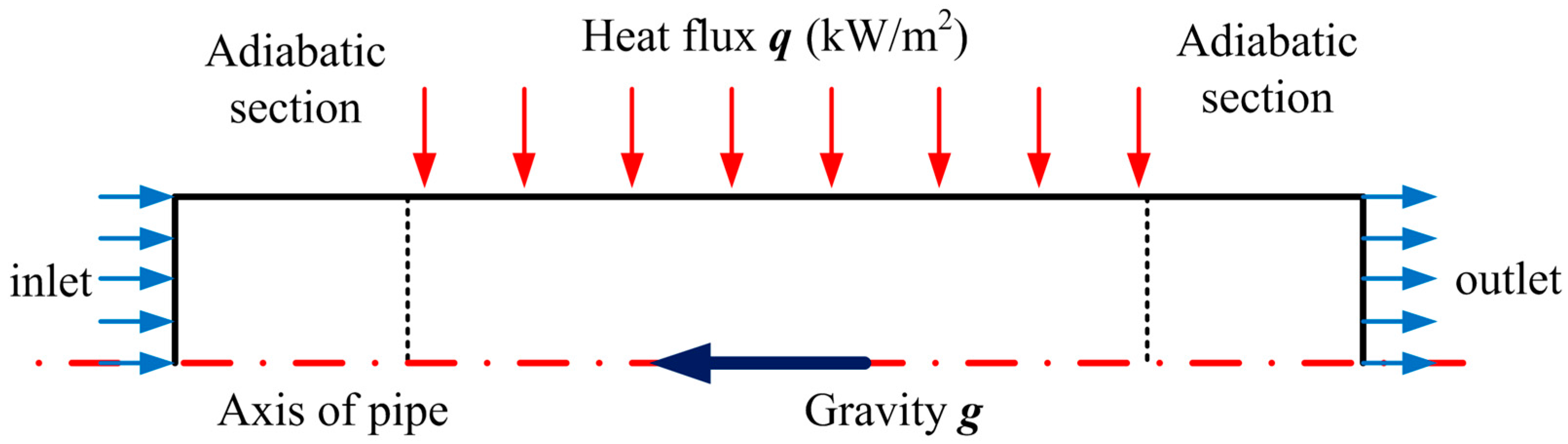
Figure 4.
2-D computational domain and boundary conditions.

Figure 5.
Variation of wall temperature in the axial direction with different meshes (q = 56.7 kW/m2).
Figure 5.
Variation of wall temperature in the axial direction with different meshes (q = 56.7 kW/m2).

Figure 6.
Variation of wall temperature (q = 56.7 kW/m2).

Figure 7.
Distribution of the axial velocity in different sections: (a) x/D = 13; (b) x/D = 26; (c) x/D = 39; and (d) x/D = 79.
Figure 7.
Distribution of the axial velocity in different sections: (a) x/D = 13; (b) x/D = 26; (c) x/D = 39; and (d) x/D = 79.

Figure 8.
Distribution of density in different sections: (a) x/D = 13; (b) x/D = 26; (c) x/D = 39; (d) x/D = 79.
Figure 8.
Distribution of density in different sections: (a) x/D = 13; (b) x/D = 26; (c) x/D = 39; (d) x/D = 79.

Figure 9.
Distribution of turbulent kinetic energy in different sections: (a) x/D = 13; (b) x/D = 26; (c) x/D = 39; (d) x/D = 79.
Figure 9.
Distribution of turbulent kinetic energy in different sections: (a) x/D = 13; (b) x/D = 26; (c) x/D = 39; (d) x/D = 79.

Figure 10.
Distribution of turbulent viscosity in different sections: (a) x/D = 13; (b) x/D = 26; (c) x/D = 39; (d) x/D = 79.
Figure 10.
Distribution of turbulent viscosity in different sections: (a) x/D = 13; (b) x/D = 26; (c) x/D = 39; (d) x/D = 79.

Figure 11.
Temperature distribution with various heat flux densities.

Figure 12.
Distribution of the axial velocity (q/G = 0.0547562).

Figure 13.
Distribution of the axial velocity (q/G = 0.0919691).

Figure 14.
Distribution of the axial velocity (x/D = 13.2).

Figure 15.
Distribution of the turbulent kinetic energy (x/D = 13.2).

Figure 16.
Distribution of the turbulent viscosity (x/D = 13.2).

Figure 17.
Distribution of the axial velocity (x/D = 26).

Figure 18.
Distribution of the turbulent kinetic energy (x/D = 26).

Figure 19.
Distribution of the turbulent viscosity (x/D = 26).

Figure 20.
Distribution of the axial velocity (x/D = 39).

Figure 21.
Distribution of the turbulent kinetic energy (x/D = 39).

Figure 22.
Distribution of the turbulent viscosity (x/D = 39).

Figure 23.
Distribution of the tube wall temperature (q = 56.7 kW/m2).

Figure 24.
Distribution of the velocity in different sections: (a) x/D = 13; (b) x/D = 26; (c) x/D = 39; (d) x/D = 53.
Figure 24.
Distribution of the velocity in different sections: (a) x/D = 13; (b) x/D = 26; (c) x/D = 39; (d) x/D = 53.

Figure 25.
Distribution of the turbulent kinetic energy in different sections: (a) x/D = 13; (b) x/D = 26; (c) x/D = 39; (d) x/D = 53.
Figure 25.
Distribution of the turbulent kinetic energy in different sections: (a) x/D = 13; (b) x/D = 26; (c) x/D = 39; (d) x/D = 53.

Figure 26.
Distribution of the turbulent viscosity in different sections: (a) x/D = 13; (b) x/D = 26; (c) x/D = 39; (d) x/D = 53.
Figure 26.
Distribution of the turbulent viscosity in different sections: (a) x/D = 13; (b) x/D = 26; (c) x/D = 39; (d) x/D = 53.


Table 1.
Analysis for the independence of the meshes.
| Item | Nodes in Axial Direction | Nodes in Radial Direction | Number |
|---|---|---|---|
| Mesh Program 1 | 600 | 60 | 35,345 |
| Mesh Program 2 | 1000 | 90 | 88,915 |
| Mesh Program 3 | 1500 | 120 | 178,385 |
| Mesh Program 4 | 2000 | 150 | 297,855 |
© 2017 by the authors. Licensee MDPI, Basel, Switzerland. This article is an open access article distributed under the terms and conditions of the Creative Commons Attribution (CC BY) license (http://creativecommons.org/licenses/by/4.0/).
Share and Cite
MDPI and ACS Style
Cai, C.; Wang, X.; Mao, S.; Kang, Y.; Lu, Y.; Han, X.; Liu, W. Heat Transfer Characteristics and Prediction Model of Supercritical Carbon Dioxide (SC-CO2) in a Vertical Tube. Energies 2017, 10, 1870. https://doi.org/10.3390/en10111870
AMA Style
Cai C, Wang X, Mao S, Kang Y, Lu Y, Han X, Liu W. Heat Transfer Characteristics and Prediction Model of Supercritical Carbon Dioxide (SC-CO2) in a Vertical Tube. Energies. 2017; 10(11):1870. https://doi.org/10.3390/en10111870
Chicago/Turabian StyleCai, Can, Xiaochuan Wang, Shaohua Mao, Yong Kang, Yiyuan Lu, Xiangdong Han, and Wenchuan Liu. 2017. "Heat Transfer Characteristics and Prediction Model of Supercritical Carbon Dioxide (SC-CO2) in a Vertical Tube" Energies 10, no. 11: 1870. https://doi.org/10.3390/en10111870
Note that from the first issue of 2016, this journal uses article numbers instead of page numbers. See further details here.