Fuzzy Logic Based MPPT Controller for a PV System

Abstract

The output power of a photovoltaic (PV) module depends on the solar irradiance and the operating temperature; therefore, it is necessary to implement maximum power point tracking controllers (MPPT) to obtain the maximum power of a PV system regardless of variations in climatic conditions. The traditional solution for MPPT controllers is the perturbation and observation (P&O) algorithm, which presents oscillation problems around the operating point; the reason why improving the results obtained with this algorithm has become an important goal to reach for researchers. This paper presents the design and modeling of a fuzzy controller for tracking the maximum power point of a PV System. Matlab/Simulink (MathWorks, Natick, MA, USA) was used for the modeling of the components of a 65 W PV system: PV module, buck converter and fuzzy controller; highlighting as main novelty the use of a mathematical model for the PV module, which, unlike diode based models, only needs to calculate the curve fitting parameter. A P&O controller to compare the results obtained with the fuzzy control was designed. The simulation results demonstrated the superiority of the fuzzy controller in terms of settling time, power loss and oscillations at the operating point.

1. Introduction

In recent years, the use of photovoltaic (PV) energy has experienced significant progress as an alternative to solve energy problems in places with high solar density, which is due to pollution caused by fossil fuels and the constant decrease of prices of the PV modules. Unfortunately, the energy conversion efficiency of the PV modules is low, which reduces the cost-benefit ratio of PV systems.

The maximum power that a PV module can supply is determined by the product of the current and the voltage at the maximum power point, which depends on the operating temperature and the solar irradiance. The short-circuit current of a PV module is directly proportional to the solar irradiance, decreasing considerably as the irradiation decreases, while the open circuit voltage varies moderately due to changes in irradiation. In contrast, the voltage decreases considerably when the temperature increases, while the short circuit current increases moderately.

In summary, increases in solar irradiation produce increases in the short-circuit current, while increases in temperature decrease the open circuit voltage, which affects the output power of the PV module. This variability of the output power means that in the absence of a coupling device between the PV module and the load, the system does not operate at the maximum power point (MPP).

According to the previous context, the use of maximum power point (MPPT) controllers is currently increasing [1]. These devices are responsible for regulating the charge of the batteries, controlling the point at which the PV modules produces the greatest amount of energy possible, regardless of variations in climatic conditions. The use of MPPT controllers in PV systems has the following advantages: 1. They yield more power, depending on weather and temperature; 2. They allow the connection of PV modules in series to increase the voltage of the system, which reduces the wiring gauge and adds flexibility; 3. They offer a cost savings in the transmission wire needed for the installation of the PV system.

In contrast to MPPT controllers, traditional controllers make a direct connection of the PV modules to the batteries, which requires that the modules operate in a voltage range that is below to the voltage in maximum power point. For example, in the case of a 12 V system, the battery voltage can vary between 11 V and 15 V, but the voltage at the maximum power point is a typical value between 16 V and 17 V. Due to this situation, with the traditional controllers the energy that the PV modules can deliver is not maximized.

Taking into account the above, different researches have been carried out using traditional algorithms for the modeling and implementation of MPPT controllers [2], of which the following are highlighted: perturb and observe (P&O) [3,4], modified P&O [5,6], fractional short circuit current [7], fractional open circuit voltage [8], sliding mode control [9,10] and incremental conductance [11]. The P&O algorithm has been used traditionally, but it has been shown that this method has problems for tracking the MPP when there are sudden changes in solar irradiance [12].

Also, algorithms based on artificial intelligence techniques such as fuzzy logic [13,14,15,16,17,18,19] and neural networks [20,21,22] have been used, as well as the implementation of optimization algorithms such as glowworm swarm [23], ant colony [24,25] and bee colony [26,27,28]. These algorithms are part of soft computing techniques and have the advantage of being easily implemented using embedded systems. Additionally, MPPT controllers are widely used in hybrid power systems, in which different control techniques based on neural networks, fuzzy logic and particle swarm optimization have been evaluated. In [29,30,31], the effectiveness of these control techniques was demonstrated in order to achieve a fast and stable response for real power control and power system applications. The implementation of new control and optimization techniques that are detailed in [32,33,34,35] for electrical power and energy systems can be studied in the modeling and implementation of MPPT controllers.

This paper presents the design and modeling of a fuzzy controller to track the maximum power point of a PV module, using the characteristics of fuzzy logic to represent a problem through linguistic expressions [36]. This paper presents as a novelty the use of the mathematical model proposed in [37,38] for modeling the PV module, which, unlike diode based models, only needs to calculate the curve fitting parameter. The results were compared with the P&O controller, which demonstrated that the proposed approach presents less energy losses and ensures MPP in all cases evaluated in simulation. It is worth mentioning that this work is part of a set of intelligent control techniques being evaluated in the research group Magma Ingeniería of the Universidad del Magdalena in order to implement a MPPT controller of low cost and high efficiency.

The main objective of this work is the design, modeling and simulation of a fuzzy logic controller and a dc-dc converter for an off-grid PV system. In a second stage, the fuzzy logic controller will be implemented using the low-cost Arduino platform [38], taking as a reference the input variables, output, fuzzification, inference system and defuzzification evaluated during the modeling stage. The dc-dc converter will also be implemented according to the design conditions evaluated in the simulations.

This work is structured as follows: Section 2 presents the design and modeling of PV system. Section 3 shows the simulation results for different operating conditions established in Matlab-Simulink. Finally, Section 4 summarizes the main conclusions.

2. Design and Modeling of PV System

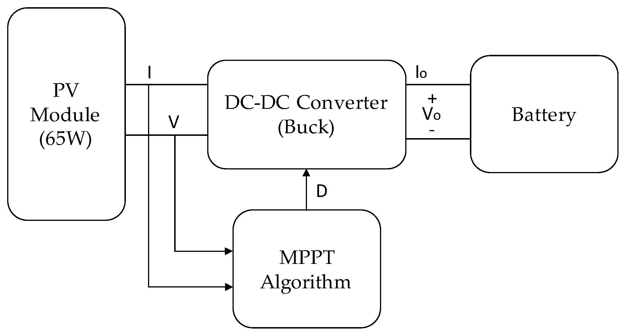
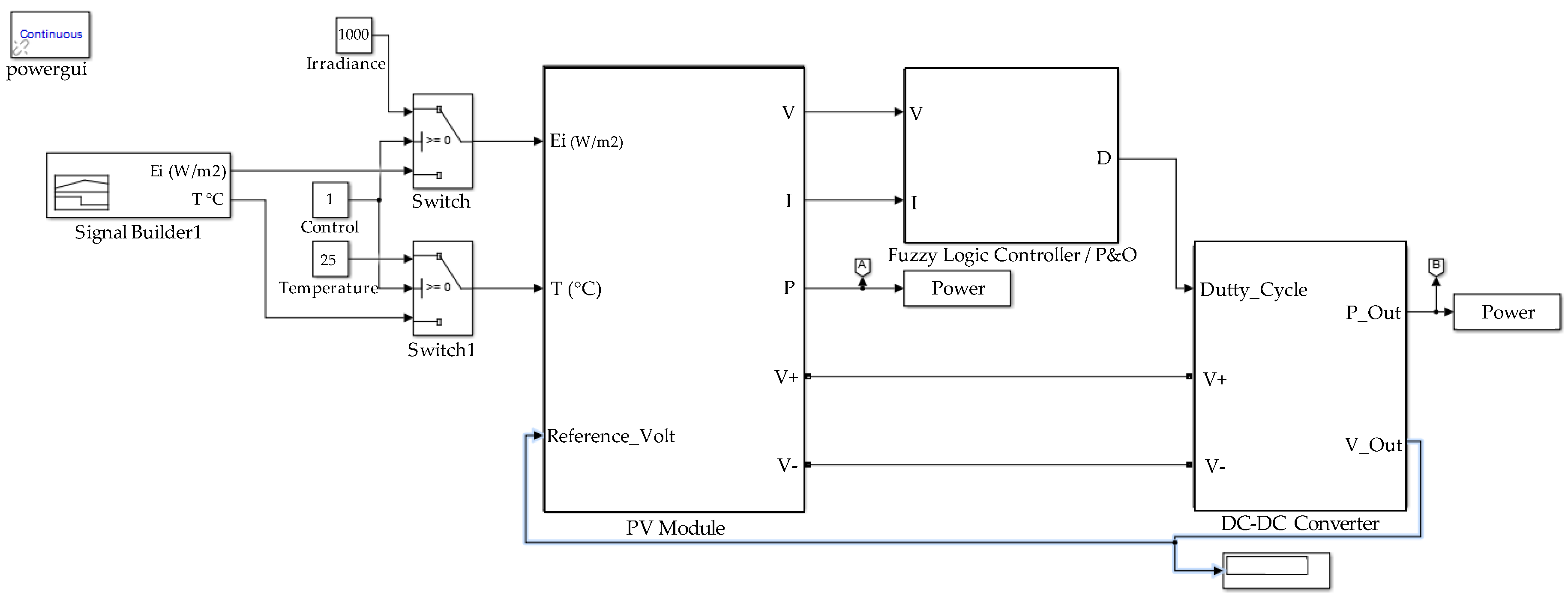
Figure 1 shows the general diagram of the PV system, which is composed of the 65 W PV module, the buck converter, the battery and the MPPT algorithm (fuzzy or P&O).

2.1. Modeling of the PV Module

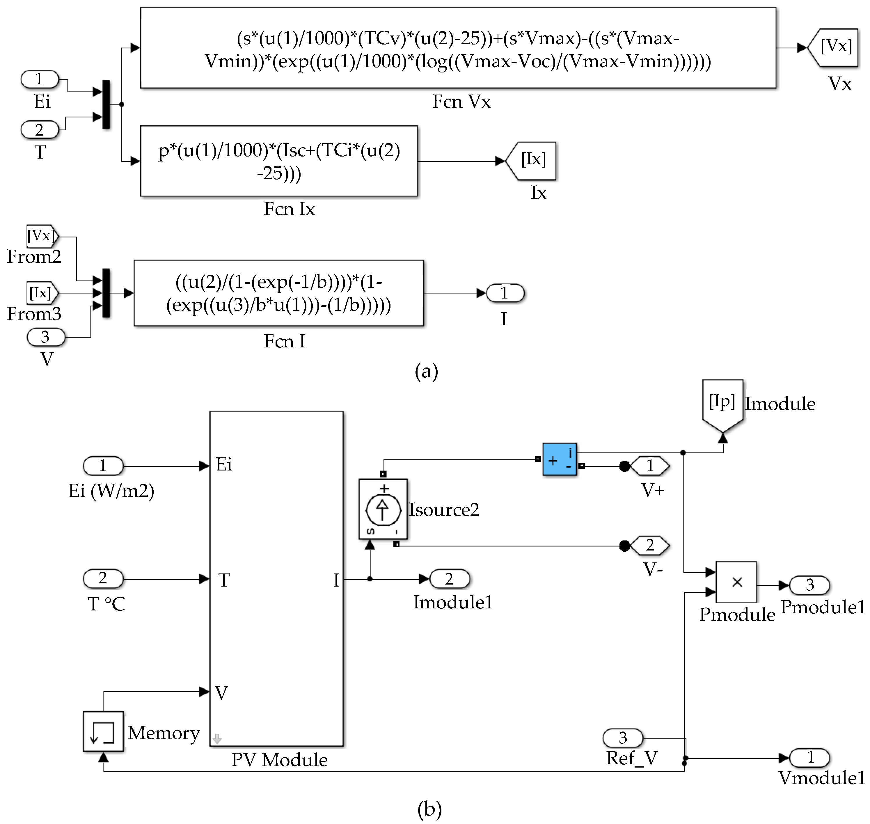
In Equation (1) the mathematical model of the PV module is shown [37,38]. With this model, it is only necessary to calculate the curve fitting parameter that can be obtained directly from the Equation (1). The other parameters are obtained from the electrical data of the PV module.

$$\mathrm{I}\left(\mathrm{V}\right)=\frac{{\mathrm{I}}_{\mathrm{x}}}{1-{\mathrm{e}}^{\left(\frac{-1}{\mathrm{b}}\right)}}\left[1-{\mathrm{e}}^{\left(\frac{\mathrm{V}}{{\mathrm{bV}}_{\mathrm{x}}}-\frac{1}{\mathrm{b}}\right)}\right]$$

(1)

where V_x and I_x are the open circuit voltage and short circuit current with dynamic values for solar irradiance and temperature, which are defined by Equations (2) and (3); b is the characteristic constant, it does not have units and is the unique parameter that has to be calculated.

$${\mathrm{V}}_{\mathrm{x}}=\mathrm{s}\frac{{\mathrm{E}}_{\mathrm{i}}}{{\mathrm{E}}_{\mathrm{iN}}}{\mathrm{TC}}_{\mathrm{v}}\left(\mathrm{T}-{\mathrm{T}}_{\mathrm{N}}\right)+{\mathrm{sV}}_{\max }-\mathrm{s}\left({\mathrm{V}}_{\max }-{\mathrm{V}}_{\min }\right){\mathrm{e}}^{\left(\frac{{\mathrm{E}}_{\mathrm{i}}}{{\mathrm{E}}_{\mathrm{iN}}}\ln \left(\frac{{\mathrm{V}}_{\max }-{\mathrm{V}}_{\mathrm{oc}}}{{\mathrm{V}}_{\max }-{\mathrm{V}}_{\min }}\right)\right)}$$

(2)

$${\mathrm{I}}_{\mathrm{x}}=\mathrm{p}\frac{{\mathrm{E}}_{\mathrm{i}}}{{\mathrm{E}}_{\mathrm{iN}}}\left[{\mathrm{I}}_{\mathrm{sc}}+{\mathrm{TC}}_{\mathrm{i}}\left(\mathrm{T}-{\mathrm{T}}_{\mathrm{N}}\right)\right]$$

(3)

where; s: number of PV modules connected in series; p: number of PV modules connected in parallel; E_i: effective irradiation of the PV module; E_iN: irradiation constant of 1000 W/m²; T: temperature of the PV module; T_N: temperature constant of 25 °C; T_cv: temperature coefficient of voltage; T_ci: temperature coefficient of current; V_oc: open circuit voltage; I_sc: short-circuit current; V_max: voltage for irradiations under 200 W and operating temperature of 25 °C (this value is 103% of V_oc); V_min: voltage for irradiations over 1200 W and operating temperature of 25 °C (this value is 85% of V_oc).

The electrical parameters of the 65 W PV module (Yingli Solar, Baoding, China) are illustrated in

Table 1. Electrical parameters of the PV module type YL65P-17b.

Parameter	Value
Short-circuit current (Isc)	4 A
Open circuit voltage (Voc)	21.7 V
Voltage at Pmax (Vmpp)	17.5 V
Current at Pmax (Impp)	3.71 A
Temperature coefficient of voltage (Tcv)	−0.0802 V/°C
Temperature coefficient of current (Tci)	0.0024 A/°C
Maximum voltage (Vmax)	22.35 V
Minimum voltage (Vmin)	18.44 V

. To find b, Equation (1) and the parameters of Table 1 were used. Knowing that the value of b is in the range of 0.01 to 0.18 [39], the approximation of Equation (4) can be done.

$$1-{\mathrm{e}}^{\left(\frac{-1}{\mathrm{b}}\right)}\approx 1$$

(4)

Therefore, for V_x = 21.7 V; I_x = 4 A; I = 3.71 A and V = 17.5 V; the value of b is 0.07375.

Figure 2a shows the modeling of the PV module with the Simulink function blocks (MathWorks, Natick, MA, USA). Figure 2b presents the PV module in a subsystem, which was evaluated for different values of solar irradiance and temperature.

Table 2. Parameters of the PV module for variable solar irradiance.

Parameter	1000 W/m2	800 W/m2	600 W/m2	400 W/m2	200 W/m2
Short-circuit current Isc (A)	4.0	3.2	2.4	1.6	0.8
Open circuit voltage Voc (V)	21.70	21.42	21.02	20.44	19.62
Voltage at Pmax Vmpp (V)	17.66	17.55	17.37	16.78	16.08
Current at Pmax Impp (A)	3.679	2.924	2.171	1.459	0.730
Maximum Power Point (W)	64.98	51.31	37.72	24.48	11.75

shows the values obtained with the mathematical model of the PV module, using variable solar irradiance and operating temperature of 25 °C. It can be seen that the values obtained for standard test conditions (E_i = 1000 W/m², T = 25 °C) correspond to the electrical parameters of the PV module presented in Table 1. Additionally, it is worth noting that the decreases in the solar irradiance considerably affect the short-circuit current, while the open circuit voltage is affected in smaller proportion.

Table 3. Parameters of the PV module for variable temperature.

Parameter	0 °C	25 °C	50 °C	75 °C
Short-circuit current Isc (A)	3.94	4.00	4.06	4.12
Open circuit voltage Voc (V)	23.71	21.7	19.69	17.69
Voltage at Pmax Vmpp (V)	19.39	17.66	16.47	14.47
Current at Pmax Impp (A)	3.606	3.679	3.617	3.771
Maximum Power Point (W)	69.92	64.98	59.59	54.55

shows the data obtained with the mathematical modeling of the PV module for solar irradiance of 1000 W/m² and variable temperature. In this case, it can be noted that increases in temperature considerably affect the open circuit voltage, while the short-circuit current is affected in a smaller proportion. Table 2 and Table 3 will be used as references in the results and discussion section, in which a comparison with the fuzzy and P&O controllers will be made; with variations of the solar irradiance and the operating temperature of the PV module.

2.2. DC-DC Converter Model

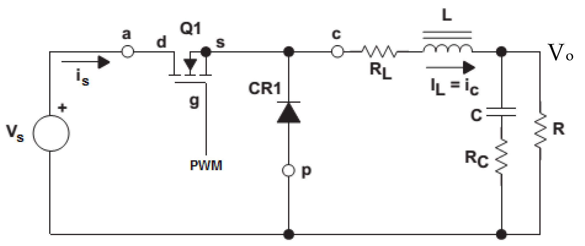
A buck converter as control device was used. Figure 3 shows the circuit that was designed to ensure that the converter operates in the continuous conduction mode (CCM); in order to avoid that, the current in the inductor reaches zero during a time interval.

In the CCM, when the transistor is conducting, the diode is in open circuit (T_on). Using Equation (5), the ripple of the inductor is obtained as shown in Equation (6).

$${\mathrm{V}}_{\mathrm{L}}=\frac{{\mathrm{L}\Delta \mathrm{I}}_{\mathrm{L}}}{\Delta \mathrm{t}}$$

(5)

$$\Delta {\mathrm{I}}_{\mathrm{L}}(+)=\frac{({\mathrm{V}}_{\mathrm{s}}-{\mathrm{V}}_{\mathrm{DS}}-{\mathrm{I}}_{\mathrm{L}}{\mathrm{R}}_{\mathrm{L}})-{\mathrm{V}}_{\mathrm{o}}}{\mathrm{L}}{\mathrm{T}}_{\mathrm{on}}$$

(6)

The inductor current decreases during the off state as shown in Equation (7).

$$\Delta {\mathrm{I}}_{\mathrm{L}}(-)=\frac{{\mathrm{V}}_{\mathrm{o}}+\left({\mathrm{V}}_{\mathrm{d}}+{\mathrm{I}}_{\mathrm{L}}{\mathrm{R}}_{\mathrm{L}}\right)}{\mathrm{L}}{\mathrm{T}}_{\mathrm{off}}$$

(7)

Assuming that V_d, R_L y V_DS are very small values, Equations (8) and (9) are obtained.

$$\Delta {\mathrm{I}}_{\mathrm{L}}(+)=\frac{({\mathrm{V}}_{\mathrm{s}}-{\mathrm{V}}_{\mathrm{o}})}{\mathrm{L}}{\mathrm{T}}_{\mathrm{on}}$$

(8)

$$\Delta {\mathrm{I}}_{\mathrm{L}}(-)=\frac{{\mathrm{V}}_{\mathrm{o}}}{\mathrm{L}}{\mathrm{T}}_{\mathrm{off}}$$

(9)

Equating Equations (8) and (9); using T_s = T_off + T_on, Equation (10) for the duty cycle D is obtained.

$$\mathrm{D}=\frac{{\mathrm{T}}_{\mathrm{on}}}{{\mathrm{T}}_{\mathrm{s}}}=\frac{{\mathrm{V}}_{\mathrm{o}}}{{\mathrm{V}}_{\mathrm{s}}}$$

(10)

2.2.1. Inductor Design

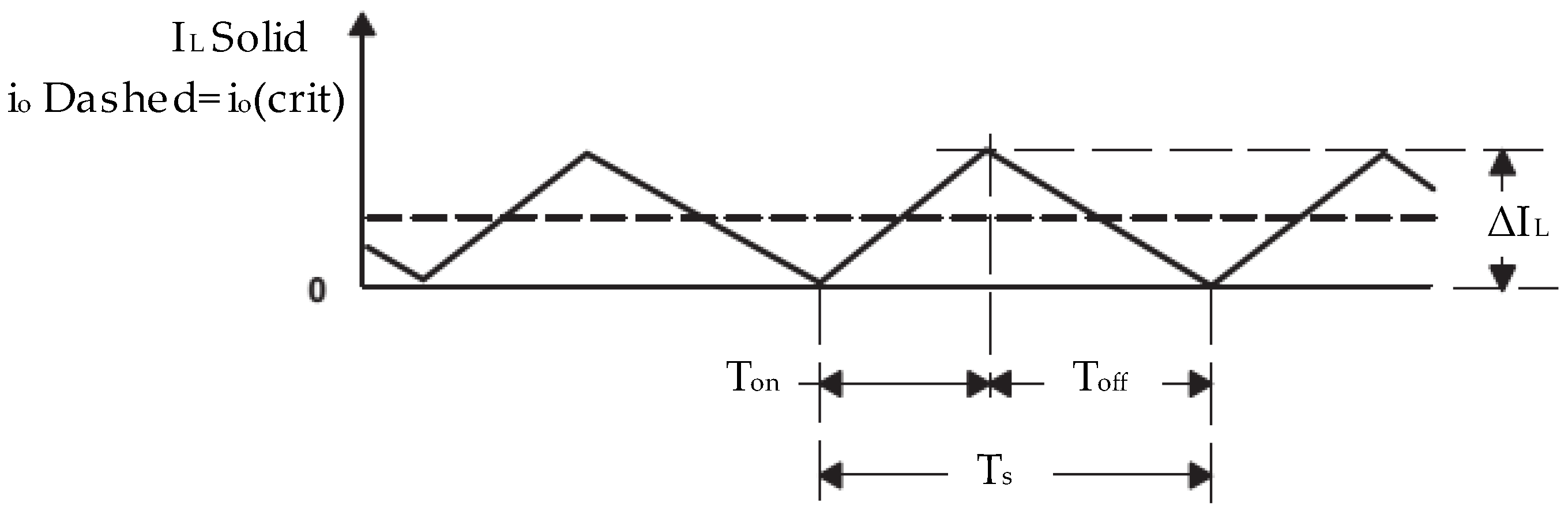
The inductor was designed to maintain the balance volts per second of the converter and to reduce ripple in the output current. Using an improper inductor produces an alternating current ripple in the direct current output, causing a change between continuous and discontinuous conduction modes. To operate in the continuous conduction mode, the critical output current must be greater than or equal to half the inductor current ripple. See Equation (11) and Figure 4.

$${\mathrm{i}}_{\mathrm{o}}\left(\mathrm{crit}\right)\ge \frac{\Delta {\mathrm{I}}_{\mathrm{L}}}{2}$$

(11)

Replacing Equation (8) in (12), using T_on = DT_s, the Equation (12) for the design of the inductor is obtained.

$${\mathrm{L}}_{\min }\ge \frac{{\mathrm{V}}_{\mathrm{o}}(1-\frac{{\mathrm{V}}_{\mathrm{o}}}{{\mathrm{V}}_{\mathrm{s}}}){\mathrm{T}}_{\mathrm{s}}}{2{\mathrm{i}}_0\left(\mathrm{crit}\right)}$$

(12)

To calculate L, the maximum power and voltage according to the MPP of the PV module were used: V_s = 17.71 V, P_max = 64.984 W, i_o = 5.41 A, f_s = 20 KHz. Using a ripple value of 10% for a maximum output current, Equation (13) is obtained.

$$\Delta {\mathrm{I}}_{\mathrm{L}}=0.1\times {\mathrm{i}}_{\mathrm{o}}\left(\max \right)=0.541\mathrm{A}$$

(13)

Using Equations (12) and (13), the minimum value of the inductor as shown in Equation (14) is obtained.

$$\mathrm{L}\ge \frac{12\times (1-\frac{12}{17.71})\times 50\mathsf{\mu }\mathrm{S}}{2\times 0.2705}\ge 357.57\mathsf{\mu }\mathrm{H}$$

(14)

2.2.2. Capacitor Design

The current in the capacitor is defined as the variation of the charge with respect to time. See Equation (15).

$$\mathrm{i}=\frac{\Delta \mathrm{Q}}{\Delta \mathrm{t}}=\mathrm{C}\frac{\Delta {\mathrm{V}}_{\mathrm{c}}}{\Delta \mathrm{t}}$$

(15)

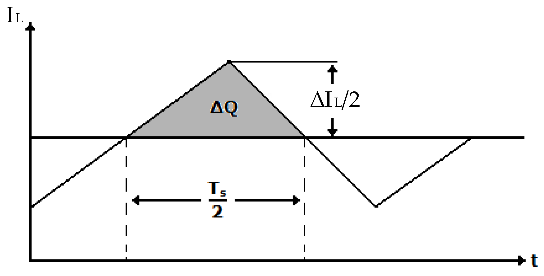
Using Figure 5 and Equation (15), the expression for the variation of the load ΔQ is obtained. See Equation (16).

$$\Delta \mathrm{Q}=\frac{\Delta {\mathrm{I}}_{\mathrm{L}}{\mathrm{T}}_{\mathrm{s}}}{8}$$

(16)

Therefore, Equation (17) for the design of the capacitor is obtained.

$$\mathrm{C}\ge \frac{\Delta {\mathrm{I}}_{\mathrm{L}}{\mathrm{T}}_{\mathrm{s}}}{8\Delta {\mathrm{V}}_{\mathrm{c}}}$$

(17)

Using a ripple value of 0.1%, Equation (18) is obtained.

$$\Delta \mathrm{V}=\left(0.001\right)\left({\mathrm{V}}_{\mathrm{o}}\right)=0.012\mathrm{V}$$

(18)

From Equations (13), (17) and (18), the minimum value of the capacitor is obtained. See Equation (19).

$$\mathrm{C}\ge \frac{\Delta {\mathrm{I}}_{\mathrm{L}}{\mathrm{T}}_{\mathrm{s}}}{8\Delta {\mathrm{V}}_{\mathrm{c}}}\ge 279.63\mathsf{\mu }\mathrm{F}$$

(19)

2.2.3. Modelling of Buck Converter

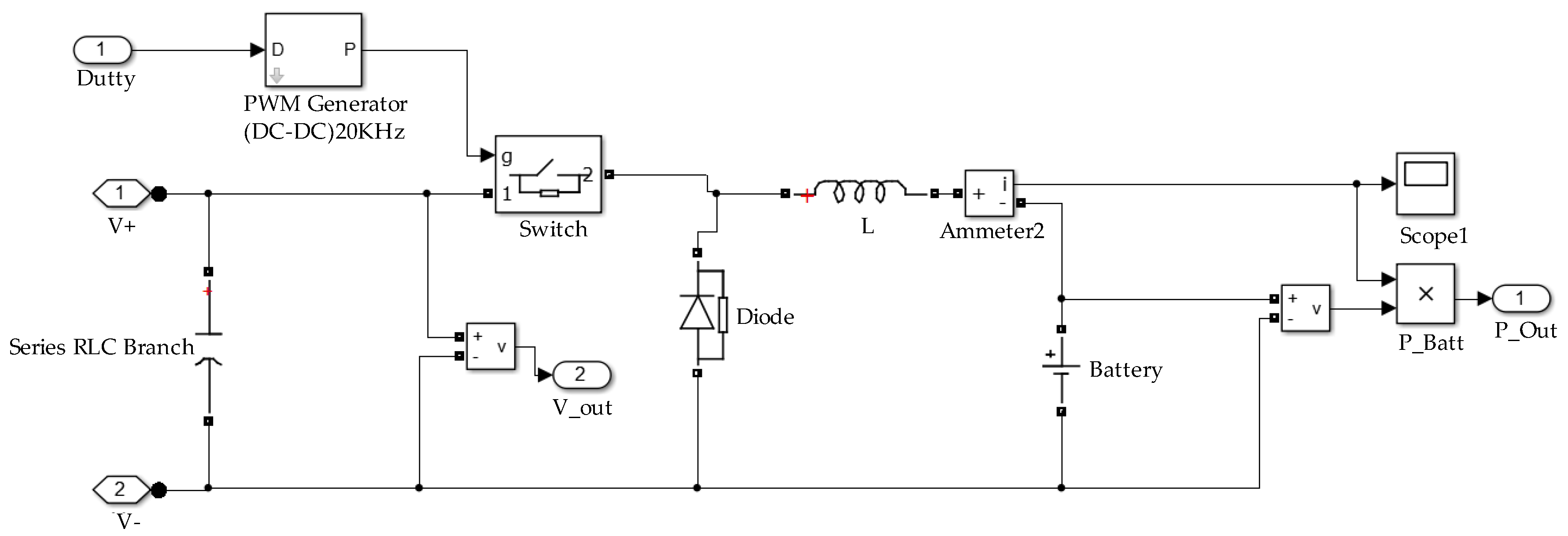
Figure 6 shows the buck converter that was modeled using the fundamental blocks of Simulink.

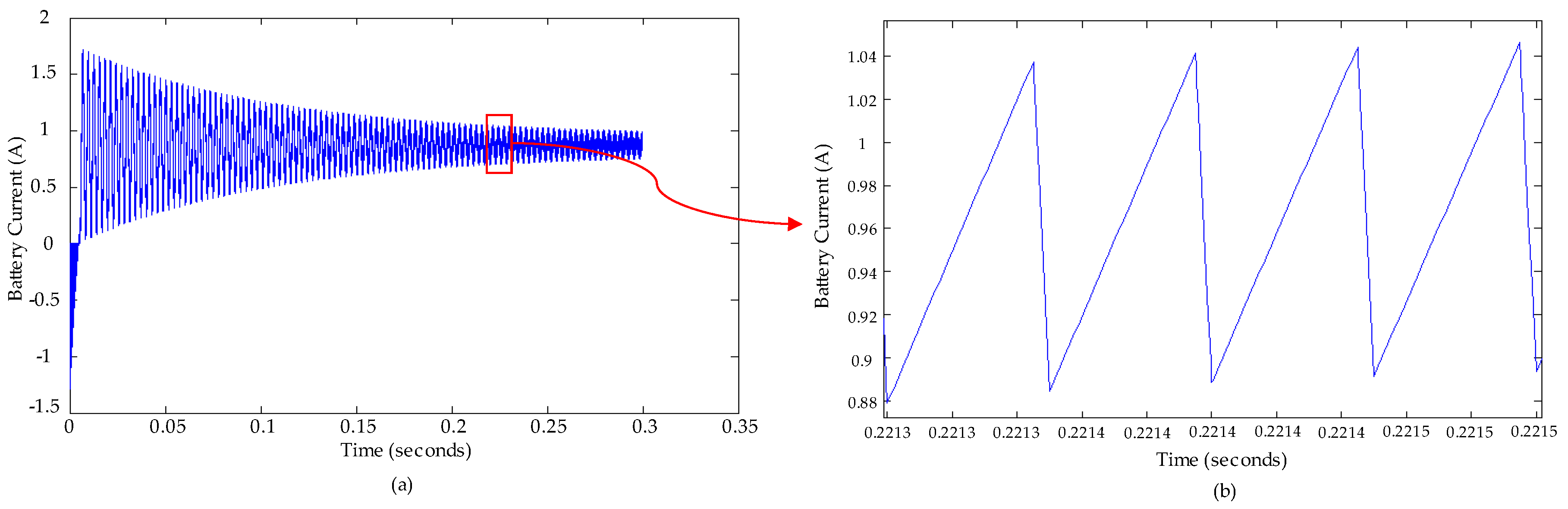
Figure 7 shows the current in the battery with the buck converter in open loop, with solar irradiance of 200 W/m² and temperature of 25 °C; in which it is observed that the converter works in the CCM according to that established in the design conditions.

2.3. Fuzzy Controller Design

Fuzzy control is a method that allows the construction of nonlinear controllers from heuristic information that comes from the knowledge of an expert. Figure 8 shows the block diagram of a fuzzy controller. The fuzzification block is responsible for processing the input signals and assign them a fuzzy value. The set of rules allows a linguistic description of the variables to be controlled and is based on the knowledge of the process. The inference mechanism is responsible for making an interpretation of the data taking into account the rules and their membership functions. With the defuzzification block, the fuzzy information coming from the inference mechanism is converted into non-fuzzy information that is useful for the process to be controlled.

Taking into account the above, the design of fuzzy controller for this work is presented. A fuzzy controller with two inputs and one output was designed. The two input variables are Error (E) and Change of Error (CE), which are shown in Equations (20) and (21) for sample times k.

$$\mathrm{E}\left(\mathrm{k}\right)=\frac{\mathrm{P}\left(\mathrm{k}\right)-\mathrm{P}\left(\mathrm{k}-1\right)}{\mathrm{V}\left(\mathrm{k}\right)-\mathrm{V}\left(\mathrm{k}-1\right)}=\frac{\Delta \mathrm{P}}{\Delta \mathrm{V}}$$

(20)

$$\mathrm{CE}\left(\mathrm{k}\right)=\mathrm{E}\left(\mathrm{k}\right)-\mathrm{E}\left(\mathrm{k}-1\right)=\Delta \mathrm{E}$$

(21)

The input E(k) is the slope of the P-V curve and defines the location of the MPP in the PV module. The CE(k) input defines whether the movement of the operating point is in the MPP direction or not. The output variable is the increment in duty cycle (ΔD), which can take positive or negative values depending on the location of the operating point. This output is sent to the dc-dc converter to drive the load. Using the value of ΔD delivered by the controller, an accumulator was made to obtain the value of the duty cycle. See Equation (22).

$$\mathrm{D}\left(\mathrm{k}\right)=\mathrm{D}\left(\mathrm{k}-1\right)+\Delta \mathrm{D}\left(\mathrm{k}\right)$$

(22)

2.3.1. Membership Functions

Triangular membership functions for the fuzzification process were used. For the inputs E, CE and for the output ΔD, 5 membership functions were defined in terms of the following linguistic variables: Very Low (MB), Low (B), Neutral (N), High (A) and Very High (MA). The range for the error is (−60 to 100), for the change of error is (−10 to 10) and for the increment in duty cycle is (−0.01 to 0.01). Figure 9 shows the membership functions for the inputs and outputs of the controller.

2.3.2. Fuzzy Rules

Table 4. Fuzzy associative matrix.

E/ΔE	Very Low	Low	Neutral	High	Very High
Very Low	VH	VH	H	VL	VL
Low	H	H	H	VL	L
Neutral	H	H	N	L	L
High	H	H	L	L	VL
Very High	H	H	L	L	VL

shows the 25 fuzzy rules applied in the controller. The rows and columns represent the two inputs E and ΔE. The output ΔD is a variable located at the intersection of a row with a column.

2.3.3. Fuzzy Controller Modelling

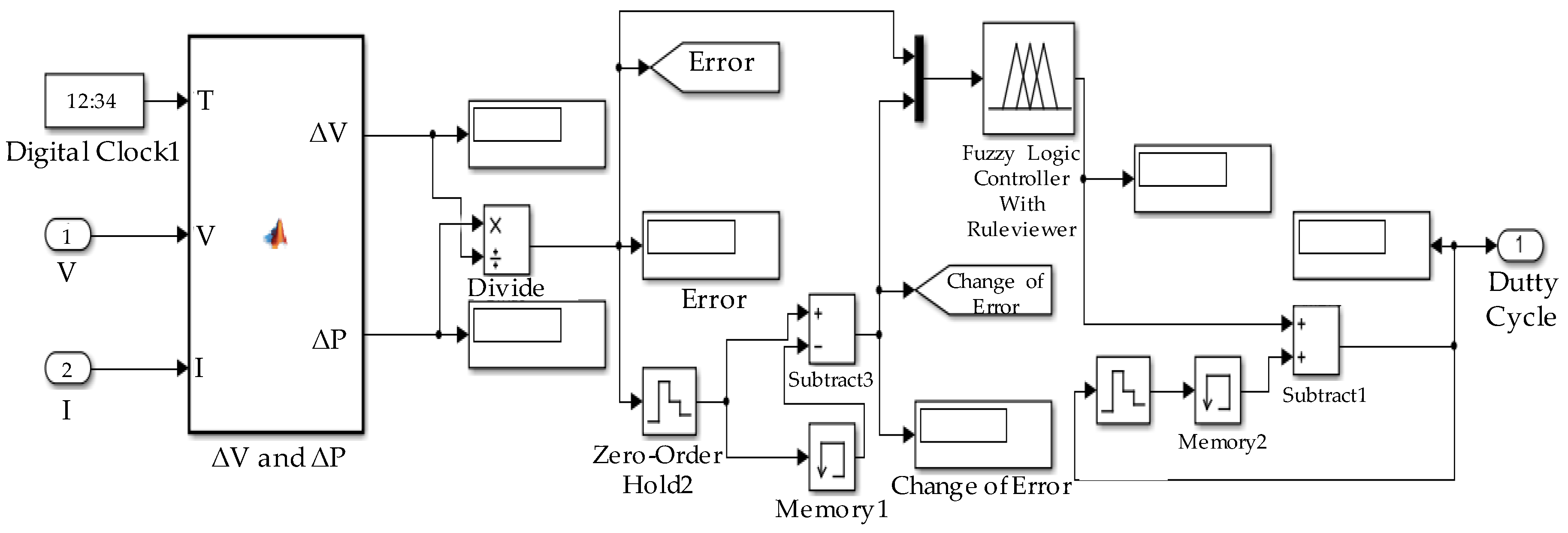
The controller was modeled with the Matlab Fuzzy Logic Toolbox (MathWorks, Natick, MA, USA). A Mamdani controller with the centroid defuzzification method was used. This procedure was carried out using the fuzzy inference system editor (FIS editor) (MathWorks, Natick, MA, USA). Figure 10 shows the controller modeled in Simulink, for which a subsystem was performed to calculate ΔV and ΔP in order to obtain the inputs E and ΔE.

2.4. P&O Controller Design

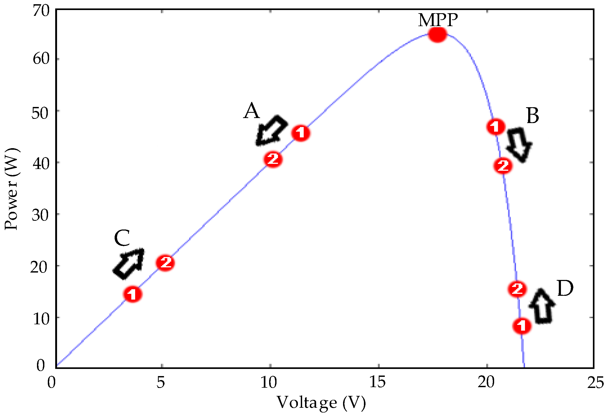
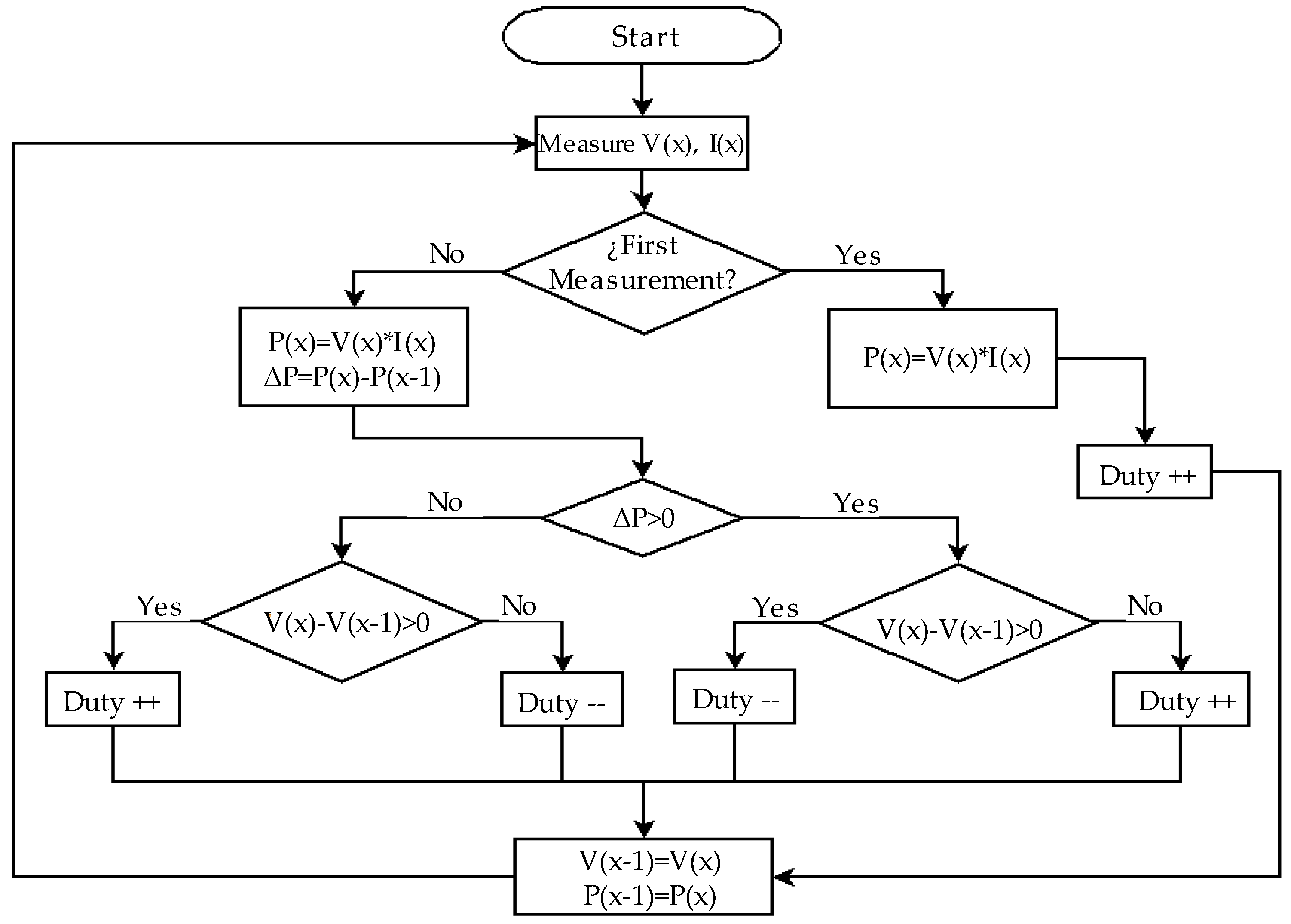
The P&O algorithm consists of modifying the operating point of the PV module by increasing or decreasing the duty cycle of a dc-dc converter in order to measure the output power before and after the perturbance. If the power increases, the algorithm perturbs the system in the same direction; otherwise the system is perturbed in the opposite direction. Figure 11 shows the 4 possible options that are presented during the tracking of the MPP, with point 1 being the previous position and point 2 being the current position of each case (A, B, C and D).

• Case A: ΔP < 0 y ΔV < 0.
• Case B: ΔP < 0 y ΔV > 0.
• Case C: ΔP > 0 y ΔV > 0.
• Case D: ΔP > 0 y ΔV < 0.

In cases A and C, the duty cycle must decrease, causing the PV module voltage to increase; while in cases B and D the duty cycle must be increased so that the voltage of the PV module decreases. The flowchart implemented for the P&O controller is shown in Figure 12.

2.5. PV System Modelling

Figure 13 shows the PV system implemented in Matlab/Simulink, which is composed of the PV module, the buck converter and the fuzzy/P&O controller. The signal builder block was used to generate the temperature and irradiance signals in order to evaluate the controller performance. Additionally, this system was used to evaluate the standard P&O controller and perform the comparison with the fuzzy controller.

2.6. Limitations

The dc-dc converter and fuzzy control were designed based on the electrical parameters of the PV module under study; for this reason, the calculations made apply to PV modules with powers up to 65 W. One of the inputs of the fuzzy controller is the change of error, which requires a differentiation operation that increases the complexity in the calculations and can generate errors when measuring small powers that are sensitive to noise.

3. Results and Discussion

To test the performance of the PV system, different scenarios were simulated in which the traditional P&O control is evaluated in comparison with the fuzzy controller. Four scenarios that simulate sudden changes in solar irradiance and operating temperature of the PV module are presented. In all cases, the following elements were used: 65 W PV module, 12 V battery, inductor of 416 μH and capacitor of 500 μF; with a sampling frequency of 20 KHz for the dc-dc converter.

● Case 1: standard test conditions

In this case, the two controllers were evaluated for solar irradiance of 1000 W/m² and temperature of 25 °C. Figure 14a shows the results obtained for the power delivered to the battery with a simulation time of 0.03 s. It can be seen that the two controllers extract the maximum power of 65 W with a good stabilization time of 0.005 s, which is consistent with the results obtained in [15,16]. In Figure 14b, it is observed that the duty cycle of the P&O control presents small oscillations between 0.6926 and 0.7, in contrast to the fuzzy control that is stabilized at a value of D = 0.694.

● Case 2: changes in solar irradiance, temperature of 25 °C

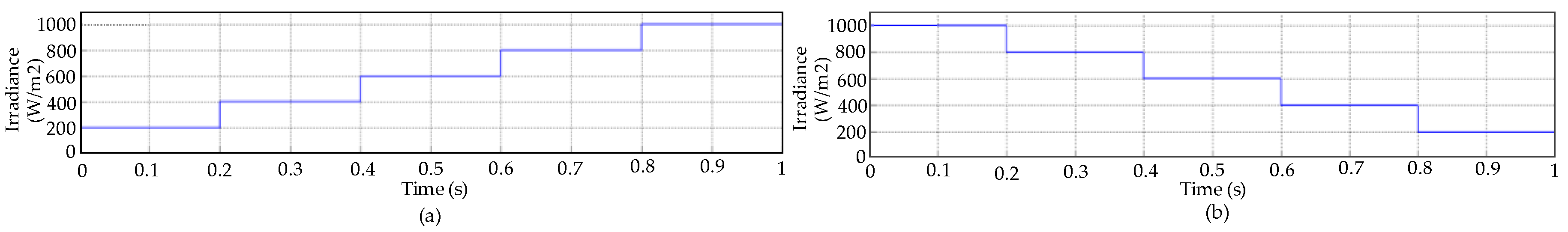
In this case, the performance of the controllers was evaluated with an operating temperature of 25 °C and sudden changes in solar irradiance. Initially, an irradiance signal was used with increments of 200 W/m², starting at 200 W/m² and ending at 1000 W/m². Changes in irradiance were made every 0.2 s with a total simulation time of 1 s (see Figure 15a). Subsequently, a test signal with decreases in solar irradiance between 1000 W/m² and 200 W/m² was used (see Figure 15b).

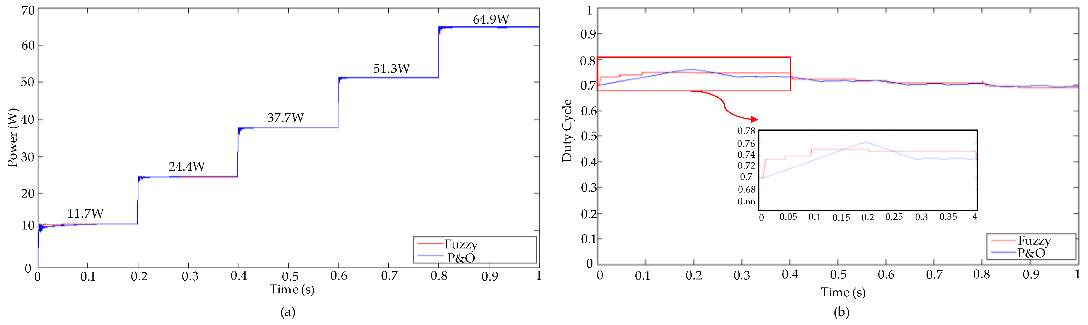
Figure 16a shows the output power for increments in the irradiance signal. In general terms it can be noted that the two controllers present a good performance in the different instants of time. The power obtained is between 11.7 W and 64.9 W, which corresponds to the values presented in Table 2. However, it should be noted that the P&O controller presented small oscillations for E_i = 200 W/m², which is evidenced in the duty cycle of Figure 16b, in times between 0 and 0.2 s.

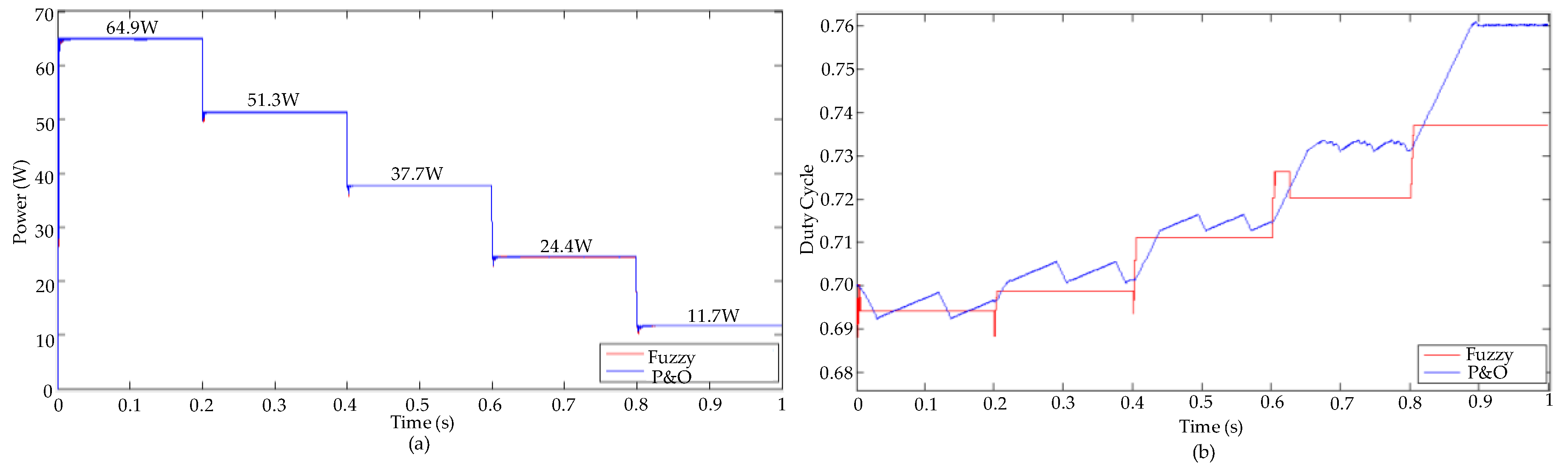
In Figure 17a, the output power for decreases in the irradiance signal is shown. As with the increase signal, the two controllers exhibit good performance with output power between 64.9 W and 11.7 W. Figure 17b shows the duty cycle, in which it is noted that the P&O controller presents the oscillations that characterize this method, but that do not significantly affect the performance of the system.

With the tests carried out in case 2, it is evident that the two controllers exhibit a similar behavior for sudden changes in solar irradiance. In addition, it was found that the P&O control has small oscillations that do not significantly affect the power delivered to the battery.

● Case 3: changes in temperature, solar irradiance of 1000 W/m²

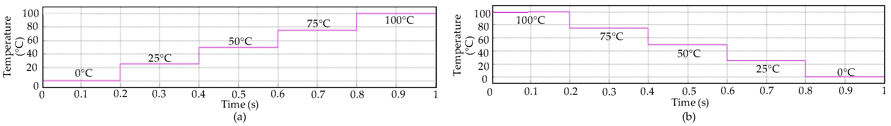
At this point, the performance of the system was evaluated for sudden changes in temperature with a constant solar irradiance of 1000 W/m². Initially, the signal shown in Figure 18a was used, with temperature increases every 0.2 s between 0 °C and 100 °C, for a test time of 1 s. Subsequently, the signal shown in Figure 18b was used, with decreases in temperature between 100 °C and 0 °C.

In Figure 19a, the power delivered to the battery is shown, where it is evident the oscillations and power losses that are obtained with the P&O control. Sudden changes in temperature significantly affect the P&O control, which is confirmed by the duty cycle signal shown in Figure 19b. In contrast, the fuzzy control delivers stable power with duty cycle values that adapt to changes in the operating temperature of the PV module. With the P&O control, there are average power losses of 3.15 W, 2.13 W, 2.84 W, 4.12 W and 6.38 W for each of the simulation intervals. The losses were calculated taking as reference the power obtained with the fuzzy controller for the five operating temperatures between 0 °C and 100 °C, which correspond to the values presented in Table 3.

Figure 20 shows the power obtained for decreases in operating temperature. As in the scenario proposed in Figure 19, the P&O control presents oscillations. The worst scenario occurs when the temperature drops from 100 °C to 75 °C, where the system does not reach stabilization and there are oscillations between 20 W and 52 W. With the P&O control, there are average power losses of 46.18 W, 17.32 W, 0 W, 1.11 W and 1.2 W.

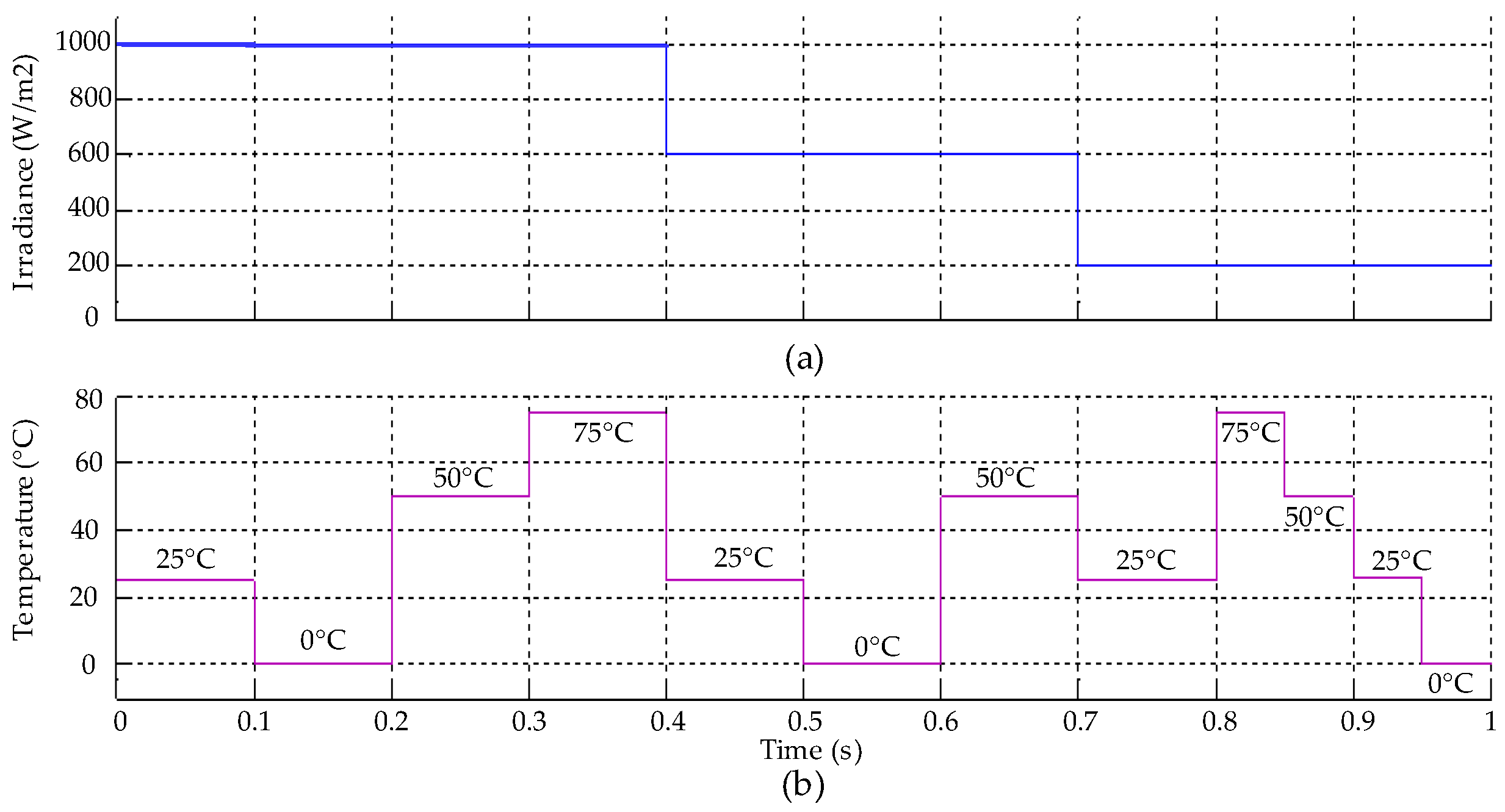
● Case 4: variations in solar irradiance and temperature

Finally, the performance of the system was evaluated for sudden changes in temperature and solar irradiance in different time values between 0 and 1 s, as seen in Figure 21.

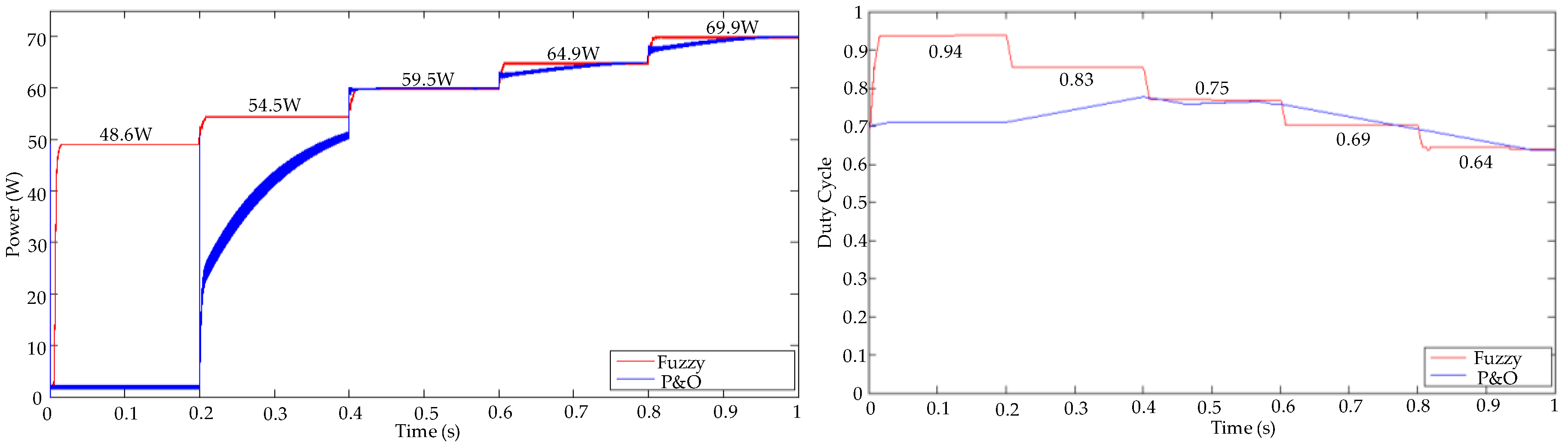
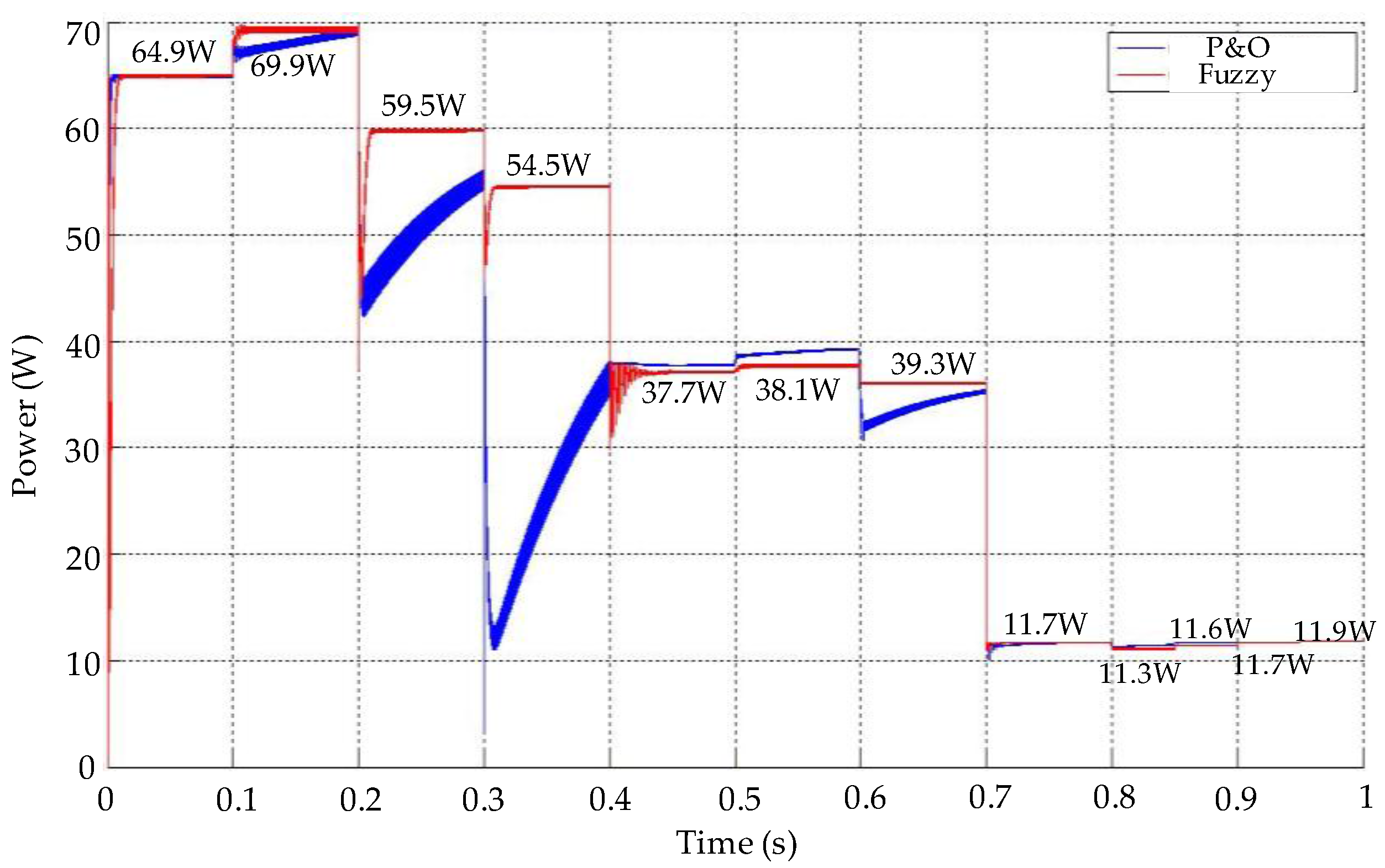
For the described test conditions, the power obtained from the PV module using fuzzy and P&O controllers is shown in Figure 22. The results prove that the fuzzy controller tracks the MPP without oscillations and power losses. In contrast, the P&O controller exhibits power losses and oscillations for changes in solar irradiance and temperature. The worst case scenario, for the P&O control, is between 0.3 and 0.4 s when the temperature changes from 50 to 75 °C with a solar irradiance of 1000 W/m^2, in which the power oscillates between 11.5 and 37.5 W. The highest average power losses with the P&O control occurred between the times 0.2 s to 0.3 s and 0.3 s to 0.4 s with values of 8.52 W and 30.48 W, respectively.

4. Conclusions

In this paper, a fuzzy controller to track the maximum power point of a PV module was presented, for which their performance was compared with a P&O controller. All components of the PV system were modeled in Matlab/Simulink (PV module, buck converter, fuzzy and P&O controllers). In this way, different test scenarios with signals of temperature and solar irradiance variables were used in order to evaluate the performance of the PV system. It was demonstrated that the fuzzy controller has an excellent performance when there are sudden changes in the operating temperature of the PV module, in contrast with P&O control that is considerably affected, presenting power losses up to 46.18 W. On the other hand, it was also evidenced that in the presence of variations in solar irradiance the two controllers presented a good performance and extracted the maximum power according to the electrical characteristics of the PV module; although the P&O control presented the well-known oscillations, mainly in the sudden changes of irradiance. In this way, the main contribution of this manuscript is the guarantee of supplying the maximum possible power to a battery in an off-grid PV system, using a fuzzy controller. As future work, in the second stage of the project, the fuzzy controller will be implemented in the low-cost Arduino platform; emphasizing that fuzzy control offers the advantage of being easily programmed in microcontrollers.

References

- Karami, N.; Moubayed, N.; Outbib, R. General review and classification of different MPPT Techniques. Renew. Sustain. Energy Rev. 2017, 68, 1–18. [Google Scholar] [CrossRef]
- Mohapatra, A.; Nayak, B.; Das, P.; Mohanty, K.B. A review on MPPT techniques of PV system under partial shading condition. Renew. Sustain. Energy Rev. 2017, 80, 854–867. [Google Scholar] [CrossRef]
- Bianconi, E.; Calvente, J.; Giral, R.; Mamarelis, E.; Petrone, G.; Ramos, C.A.; Spagnuolo, G.; Vitelli, M. Perturb and Observe MPPT algorithm with a current controller based on the sliding mode. Int. J. Electr. Power 2013, 44, 346–356. [Google Scholar] [CrossRef]
- Chen, M.; Ma, S.; Wu, J.; Huang, L. Analysis of MPPT Failure and Development of an Augmented Nonlinear Controller for MPPT of Photovoltaic Systems under Partial Shading Conditions. Appl. Sci. 2017, 7, 95. [Google Scholar] [CrossRef]
- Kwan, T.H.; Wu, X. High performance P&O based lock-on mechanism MPPT algorithm with smooth tracking. Sol. Energy 2017, 155, 816–828. [Google Scholar] [CrossRef]
- Alik, R.; Jusoh, A. Modified Perturb and Observe (P&O) with checking algorithm under various solar irradiation. Sol. Energy 2017, 148, 128–139. [Google Scholar] [CrossRef]
- Bounechba, H.; Bouzid, A.; Snani, A.; Lashab, A. Real time simulation of MPPT algorithms for PV energy system. Int. J. Electr. Power 2016, 83, 67–78. [Google Scholar] [CrossRef]
- Huang, Y.P.; Hsu, S.Y. A performance evaluation model of a high concentration photovoltaic module with a fractional open circuit voltage-based maximum power point tracking algorithm. Comput. Electr. Eng. 2016, 51, 331–342. [Google Scholar] [CrossRef]
- Cortajarena, J.A.; Barambones, O.; Alkorta, P.; De Marcos, J. Sliding mode control of grid-tied single-phase inverter in a photovoltaic MPPT application. Sol. Energy 2017, 155, 793–804. [Google Scholar] [CrossRef]
- Tobón, A.; Peláez-Restrepo, J.; Villegas-Ceballos, J.P.; Serna-Garcés, S.I.; Herrera, J.; Ibeas, A. Maximum Power Point Tracking of Photovoltaic Panels by Using Improved Pattern Search Methods. Energies 2017, 10, 1316. [Google Scholar] [CrossRef]
- Loukriz, A.; Haddadi, M.; Messalti, S. Simulation and experimental design of a new advanced variable step size Incremental Conductance MPPT algorithm for PV systems. ISA Trans. 2016, 62, 30–38. [Google Scholar] [CrossRef] [PubMed]
- Mellit, A.; Rezzouk, H.; Messai, A.; Medjahed, B. FPGA-based real time implementation of MPPT-controller for photovoltaic systems. Renew. Energy 2011, 36, 1652–1661. [Google Scholar] [CrossRef]
- Ramalu, T.; Mohd Radzi, M.A.; Mohd Zainuri, M.A.A.; Abdul Wahab, N.I.; Abdul Rahman, R.Z. A Photovoltaic-Based SEPIC Converter with Dual-Fuzzy Maximum Power Point Tracking for Optimal Buck and Boost Operations. Energies 2016, 9, 604. [Google Scholar] [CrossRef]
- Hassan, S.Z.; Li, H.; Kamal, T.; Arifoğlu, U.; Mumtaz, S.; Khan, L. Neuro-Fuzzy Wavelet Based Adaptive MPPT Algorithm for Photovoltaic Systems. Energies 2017, 10, 394. [Google Scholar] [CrossRef]
- Nabipour, M.; Razaz, M.; Seifossadat, S.; Mortazavi, S. A new MPPT scheme based on a novel fuzzy approach. Renew. Sustain. Energy Rev. 2017, 74, 1147–1169. [Google Scholar] [CrossRef]
- Bendib, B.; Krim, F.; Belmili, H.; Almi, M.F.; Boulouma, S. Advanced Fuzzy MPPT Controller for a Stand-alone PV System. Energy Procedia 2014, 50, 383–392. [Google Scholar] [CrossRef]
- Belaidi, R.; Haddouche, A.; Fathi, M.; Larafi, M.M.; Kaci, G.M. Performance of grid-connected PV system based on SAPF for power quality improvement. In Proceedings of the International Renewable and Sustainable Energy Conference (IRSEC), Marrakech, Morocco, 14–17 November 2016; pp. 1–4. [Google Scholar]
- Chekired, F.; Larbes, C.; Rekioua, D.; Haddad, F. Implementation of a MPPT fuzzy controller for photovoltaic systems on FPGA circuit. Energy Procedia 2011, 6, 541–549. [Google Scholar] [CrossRef]
- Na, W.; Chen, P.; Kim, J. An Improvement of a Fuzzy Logic-Controlled Maximum Power Point Tracking Algorithm for Photovoltic Applications. Appl. Sci. 2017, 7, 326. [Google Scholar] [CrossRef]
- Messaltia, S.; Harrag, A.; Loukriz, A. A new variable step size neural networks MPPT controller: Review, simulation and hardware implementation. Renew. Sustain. Energy Rev. 2017, 68, 221–233. [Google Scholar] [CrossRef]
- Dounis, A.I.; Kofinas, P.; Papadakis, G.; Alafodimos, C. A direct adaptive neural control for maximum power point tracking of photovoltaic system. Sol. Energy 2015, 115, 145–165. [Google Scholar] [CrossRef]
- Muthuramalingam, M.; Manoharan, P.S. Comparative analysis of distributed MPPT controllers for partially shaded stand alone photovoltaic systems. Energy Convers. Manag. 2014, 86, 286–299. [Google Scholar] [CrossRef]
- Jin, Y.; Hou, W.; Li, G.; Chen, X. A Glowworm Swarm Optimization-Based Maximum Power Point Tracking for Photovoltaic/Thermal Systems under Non-Uniform Solar Irradiation and Temperature Distribution. Energies 2017, 10, 541. [Google Scholar] [CrossRef]
- Titri, S.; Larbes, C.; Toumi, K.Y.; Benatchba, K. A new MPPT controller based on the Ant colony optimization algorithm for Photovoltaic systems under partial shading conditions. Appl. Soft Comput. 2017, 58, 465–479. [Google Scholar] [CrossRef]
- Jiang, L.L.; Maskell, D.L.; Patra, J.C. A novel ant colony optimization-based maximum power point tracking for photovoltaic systems under partially shaded conditions. Energy Build. 2013, 58, 227–236. [Google Scholar] [CrossRef]
- Benyoucef, A.S.; Chouder, A.; Kara, K.; Silvestre, S.; Sahed, O.A. Artificial bee colony based algorithm for maximum power point tracking (MPPT) for PV systems operating under partial shaded conditions. Appl. Soft Comput. 2015, 32, 38–48. [Google Scholar] [CrossRef]
- Fathy, A. Reliable and efficient approach for mitigating the shading effect on photovoltaic module based on Modified Artificial Bee Colony algorithm. Renew. Energy 2015, 81, 78–88. [Google Scholar] [CrossRef]
- Atawi, I.E.; Kassem, A.M. Optimal Control Based on Maximum Power Point Tracking (MPPT) of an Autonomous Hybrid Photovoltaic/Storage System in Micro Grid Applications. Energies 2017, 10, 643. [Google Scholar] [CrossRef]
- Ou, T.-C.; Hong, C.-M. Dynamic operation and control of microgrid hybrid power systems. Energy 2014, 66, 314–323. [Google Scholar] [CrossRef]
- Hong, C.-M.; Ou, T.-C.; Lu, K.-H. Development of intelligent MPPT (maximum power point tracking) control for a grid-connected hybrid power generation system. Energy 2013, 50, 270–279. [Google Scholar] [CrossRef]
- Shiau, J.-K.; Wei, Y.-C.; Lee, M.-Y. Fuzzy Controller for a Voltage-Regulated Solar-Powered MPPT System for Hybrid Power System Applications. Energies 2015, 8, 3292–3312. [Google Scholar] [CrossRef]
- Ou, T.-C.; Su, W.-F.; Liu, X.-Z.; Huang, S.-J.; Tai, T.-Y. A Modified Bird-Mating Optimization with Hill Climbing for Connection Decisions of Transformers. Energies 2016, 9, 671. [Google Scholar] [CrossRef]
- Ou, T.-C. A novel unsymmetrical faults analysis for microgrid distribution systems. Electr. Power Energy Syst. 2012, 43, 1017–1024. [Google Scholar] [CrossRef]
- Ou, T.-C. Ground fault current analysis with a direct building algorithm for microgrid distribution. Electr. Power Energy Syst. 2013, 53, 867–875. [Google Scholar] [CrossRef]
- Ou, T.-C.; Lu, K.-H.; Huang, C.-J. Improvement of Transient Stability in a Hybrid Power Multi-System Using a Designed NIDC (Novel Intelligent Damping Controller). Energies 2017, 10, 488. [Google Scholar] [CrossRef]
- Robles Algarín, C.; Callejas Cabarcas, J.; Polo Llanos, A. Low-Cost Fuzzy Logic Control for Greenhouse Environments with Web Monitoring. Electronics 2017, 6, 71. [Google Scholar] [CrossRef]
- Ortiz, E. Modeling and Analysis of Solar Distributed Generation. Ph.D. Thesis, Michigan State University, Michigan, MI, USA, 2006. [Google Scholar]
- Gil, O. Modelado Y Simulación de Dispositivos Fotovoltaicos. Master’s Thesis, Universidad de Puerto Rico, San Juan, Puerto Rico, 2008. [Google Scholar]
- Robles, C.; Ospino, A.; Casas, J. Dual-Axis Solar Tracker for Using in Photovoltaic Systems. Int. J. Renew. Energy Res. IJRER 2017, 10, 137–145. [Google Scholar]
Figure 1.
Block diagram of the photovoltaic (PV) system.
Figure 2.
PV module in Matlab. (a) Model implemented with Simulink function blocks; (b) Subsystem implemented for the simulation.
Figure 3.
Buck converter circuit.
Figure 4.
Critical output current.
Figure 5.
Time variation of the current in the inductor.
Figure 6.
Buck converter modeled in Simulink.
Figure 7.
(a) Battery current for open loop; (b) Extended section for range (0.2213–0.2215 s).
Figure 8.
Block diagram for a fuzzy controller.
Figure 9.
Membership functions. (a) Error; (b) Change of error; (c) Increment of duty cycle.
Figure 10.
Fuzzy logic controller.
Figure 11.
Movement of the maximum power point on the P-V curve of the PV module.
Figure 12.
Flowchart of the perturbation and observation (P&O) controller.