Norway as a Battery for the Future European Power System—Impacts on the Hydropower System

1
SINTEF Energy Research, Sem Sælands vei 11, NO-7465 Trondheim, Norway
2
NTNU, NO-7491 Trondheim, Norway
*
Author to whom correspondence should be addressed.
Energies 2017, 10(12), 2054; https://doi.org/10.3390/en10122054
Submission received: 31 October 2017
/
Revised: 23 November 2017
/
Accepted: 24 November 2017
/
Published: 4 December 2017
(This article belongs to the Special Issue Hydropower 2017)
Abstract
:Future power production in Europe is expected to include large shares of variable wind and solar power production. Norway, with approximately half of the hydropower reservoir capacity in Europe, can contribute to balance the variability. The aim of this paper is to assess how such a role may impact the Norwegian hydropower system in terms of production pattern of the plants, changes in reservoir level and water values. The study uses a stochastic optimization and simulation model and analyses an eHighway2050 scenario combined with increases in the hydropower production capacities in Norway. The capacity increases from ca. 31 GW in the present system to 42 and 50 GW respectively. The study uses 75 years with stochastic wind, solar radiation, temperature and inflow data. The results show that the hydropower system is able to partly balance the variable production and significantly reduce the power prices for the analyzed case. The paper shows that some of the power plants utilize their increased capacity, while other plants do not due to hydrological constraints and model limitations. The paper discusses how the modelling can be further improved in order to quantify more of the potential impacts on the future power system.
1. Introduction
The European Union (EU) has set itself a long-term goal of reducing greenhouse gas emissions by 80–95% by 2050, when compared to 1990 levels. Reduction of the emissions from the energy and the power systems are very important in this case. The future power system will probably include much higher shares of renewable resources like wind, solar and hydro. Wind and solar resources are variable and hydropower can contribute to balance the variability. Hydropower differs from other renewable resources due to its large flexibility and storage capability when coupled to a reservoir. Hydropower also has extremely short response times and the ability to black start. Together with its flexibility and energy storage potential, these characteristics enables hydropower to enhance the performance of all renewable technologies and act as a “battery” that can smooth out total output from variable renewables resources [1].
In the report “Hydropower in Europe. Powering Renewables” from Eurelectric, the Union of Electricity Industries in Europe [2], the quotation is put forth: “Europe has three major renewables batteries: Norway and the Scandinavian region, the Alpine region, and, to a lesser extent, the Pyrenees. Norway has a 96% share of hydropower generation in its electricity generation portfolio, producing on average 123 TWh of electricity a year. 60–70% of the annual hydropower generation is produced from conventional storage hydropower plants. Norway has almost half of Europe’s reservoir (storage) capacity. Already today, the generation flexibility of Norway’s storage hydropower enables the integration of a high level of variable renewables (>20%) within the Nordic market, mainly from wind in the electricity system of Denmark. Norway could provide a significant back-up to the continental European electricity system”.
The use of Norwegian hydropower as a battery for balancing variable renewables in neighboring countries is also discusses in other reports, like [3]. In a press release from 13 October 2014, the EU Commission welcomed the announcement made by the Norwegian government to license the construction of two subsea cables linking Norway to Germany and United Kingdom (UK). According to the press release, the two 1400 MW subsea cables will enable the three countries to exchange electricity and use the Norwegian hydropower potential. Vice-President of the EU Commission, responsible for Energy, Günther H. Oettinger said: “This will help enormously to integrate renewable energy in North-West Europe. Germany and UK can sell renewable energy to Norway when weather conditions are such that they produce a lot and Norway can sell electricity from hydropower. This will benefit both sides and balance the system” [4].
Nearly 40% of the land area in Norway is above 600 m above sea level. Many places have a lot of precipitation. Due to the cold climate, there is limited evaporation from the lakes, i.e., it is possible to utilize most of the precipitation for hydropower production. During the last Ice Age, the glaciers created many valleys and lakes in the mountains. Those valleys and lakes have been used for hydropower reservoirs in Norway. The ice from the Ice Age also polished the mountains, so sedimentation is a limited problem [5]. Presently, Norway has more than 1000 hydropower reservoirs, and the maximum stored energy in the reservoirs is approximately 85 TWh. According to [6] the maximum storage capacity in other European countries with a significant share of hydropower are (all numbers in TWh): Austria (3.2), France (9.8), Germany (0.3), Greece (2.4), Italy (7.9), Portugal (2.6), Spain (18.4) and Switzerland (8.4). Sweden has ca. 34 TWh and Finland 5 TWh [7], i.e., the total capacity for other countries than Norway is about 90 TWh. The present total generation capacity for the Norwegian hydropower plants is ca. 31 GW. Several of the largest plants and reservoirs are located in the southwestern part of the country.
Reference [8] investigated the potential for flexible electricity production from the southwestern part of the Norwegian hydropower system. The work did not consider new reservoirs, but rather looked at existing large reservoirs where expansion of existing generation capacity and construction of new pump-storage plants is possible within present regulation and concession requirements. The study showed that nearly 20 GW additional generation and pumping capacity can be developed.
Reference [9] identified state-of-the-art related to use of Nordic hydropower for balancing and storage of variable wind and solar based power production in the future Northern European system. The paper focused on the following topics: (1) the need for balancing and storage; (2) possible further development of the Nordic power system; (3) consequences of different market solutions; (4) changes in operations of the Nordic system.
The last of the four research questions, is studied in several papers: [10,11,12,13,14]. E.g., [10] shows development of reservoir level over the years and hydro power production over the years dependent of some increase in cross-border capacities. However, one of the main conclusions in [9] was that few of the studies include both wind and solar resources and with shares which can be expected in a perspective to 2050. Thus, conclusions about operational patterns may be different with higher shares of variable resources in the power system.
Reference [15] shows that increases in Norwegian hydropower production capacity significantly impacts peak and average power prices in the future Europe. This paper is based on the same methodology as [15], but focuses on other results. While [15] focuses on the impacts for the European power system and in particular the power prices, this paper is about the impacts on the Norwegian system. It aims to show how increases of capacity influences the system in terms of changes in production pattern and reservoir operation. Paper [15] also shows that the increased capacity is seldom fully utilized. This paper aims to further explore the reasons for the limitations in utilization.
The remainder of this paper is organized as follows: Section 2 described the methodology used in the analysis, Section 3 presents the results and Section 4 discusses the results and recommend further research. Appendix A shows details about the input simulation data and Appendix B shows details about the output simulation data.
2. Methodology
The future power system in Europe is analyzed with the stochastic optimization model EMPS (EFI’s (former name of SINTEF Energy Research) Multi-area Power Market Simulator) (see Section 2.1). Assumptions about the European power system in 2050 are from the EU 7th framework project eHighway2050 scenario X-7 (100% RES) (see Section 2.2). Hourly wind and radiation data are reanalyzed data described in Section 2.3. Modelling of increases in hydropower capacities are from the Twenties project and described in Section 2.4.
2.1. The Analytic Model
The EMPS model is a stochastic optimization model that maximizes the expected total socio- economic surplus in the simulated system through the optimal dispatch of generation and transmission, given a consumption profile [16]. We chose the EMPS model because it is a well-tested model used for decades by all main actors in the Nordic power market, i.e., all large power producers, the transmission system operators (TSOs) and the regulators. To our knowledge, there are no other relevant models with such an advanced representation of the Nordic systems with long- and short-term (hydropower) storage capabilities.
There is no fuel cost for hydropower. However, with a limited amount of water available in the reservoirs as well as a season-dependent inflow, the determination of an optimal strategy for hydropower generation becomes a complex problem. The goal is to find the strategy that maximizes the expected annual operation profits, considering the climatic uncertainties. In this process, EMPS executes two phases: the strategy phase and the optimization/simulation phase. In the first phase, water values for each modeled area are calculated using stochastic dynamic programming. In the second phase, the power dispatch is optimized in each time step taking the different stochastic outcomes (climatic years) into consideration. The optimization procedure starts with calculating the optimal dispatch with hydropower aggregated to one plant and one reservoir per node/region (see Figure 1). In a next step, the aggregated production is distributed on the individual hydropower plants based on advanced heuristics. The heuristics are based on the differences between the filling and the depletion season. The filling season is in the spring, the summer and the early autumn. The reservoirs are filled up due to snow melting, rain and low demand. The depletion season is in the winter when a main part of the precipitation is snow, and the demand is high due to cold climate and electric heating. Two different rules are defined for the filling and the depletion season. In the filling season, all regulation reservoirs shall have the same risk of spillage, while during the depletion season all reservoirs shall have the same risk to be emptied. The ruled-based procedure verifies if the desired production at aggregated level is obtainable within all constraints at the detailed level. If the aggregated production is not possible taking all details in the hydropower system into consideration, the loop continues with a new dispatch at aggregated level and a new reservoir drawdown procedure etc. The reservoir drawdown procedure makes a distinction between two types of reservoirs:
- Buffer reservoirs that are run according to rule curves
- Regulation reservoirs that are run according to a rule based procedure for allocation of the stored energy in the system.
Buffer reservoirs are not part of the rule-based strategy, but are filled and depleted according to their individual input rule curves. The water values and the individual target reservoirs are decided on a weekly basis, while the optimal power dispatch is calculated with user specified temporal resolution within each week.
The main inputs to the model include costs and capacities of generation, transmission and electricity consumption and information about historical climate variables like temperatures, hydro inflow, wind, solar radiation, typically with hourly resolution. The output from the model includes among other power balances and (spot) power prices.
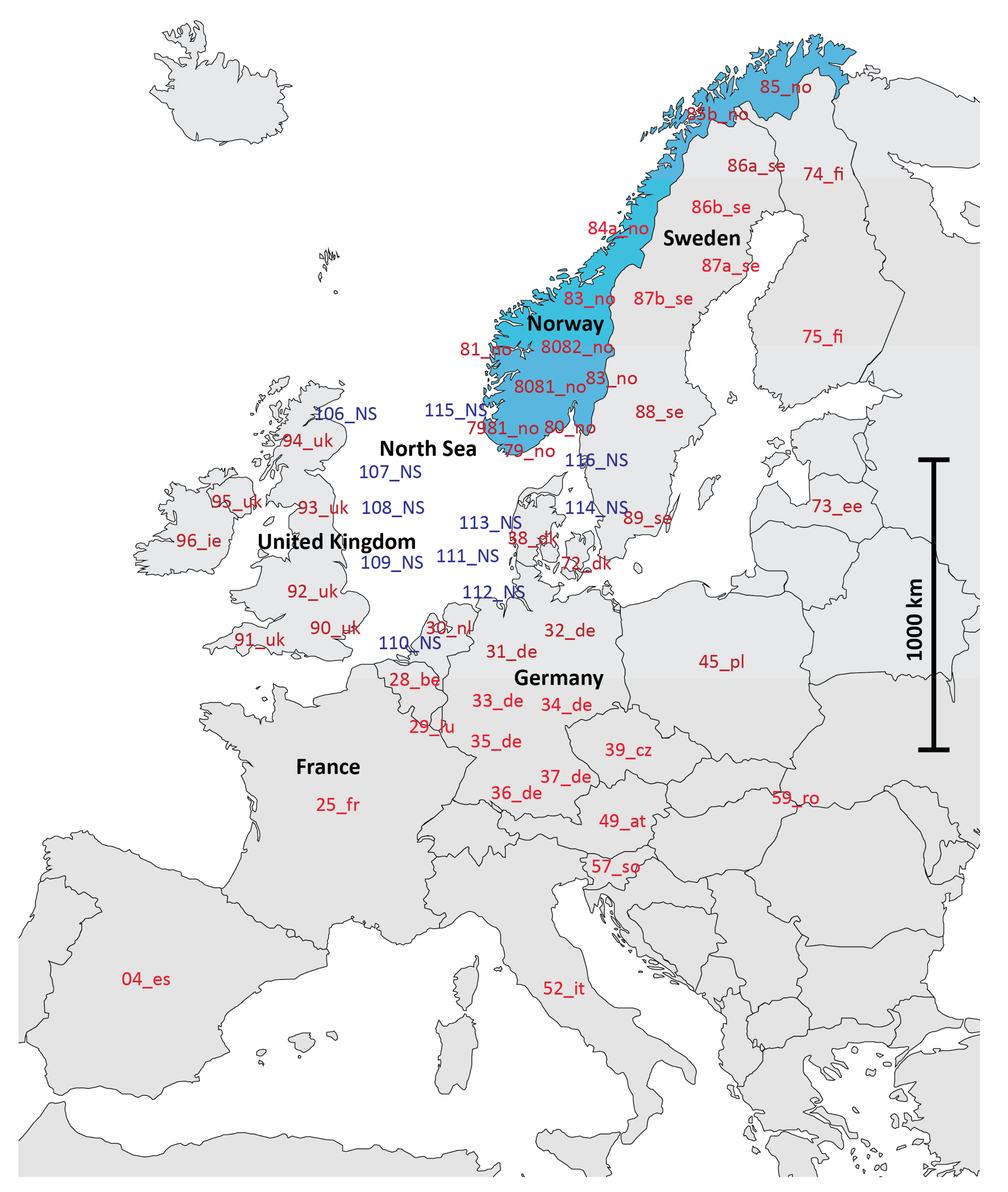
Figure 1 shows the 59 nodes/regions used in the EMPS analysis. The red text is nodes representing aggregated onshore production and consumption in the power system analysis with the EMPS model. The blue text are nodes representing aggregated offshore wind power production. The black text is only for additional information to the reader and are not used in the EMPS analysis. Each node has an endogenously determined internal supply and demand balance with distinct import and export transmission capacities to the neighboring nodes. Appendix A shows the assumptions about installed production capacities, demand and transmission capacities for each of the nodes in the figure. Appendix B shows the energy balance for each of the nodes. As shown in the figure, the Nordic countries, UK and Germany are modelled with several nodes, while Southeastern Europe is aggregated to one node (59_ro in Figure 1). The hydropower in the Nordic area include complex river systems with multiple power plants in series or parallel with 75 years of historical hydrological inflow data. Each hydropower plant and each reservoir is modelled in detail. Except for Sweden, the other European countries use a simpler hydropower model.
The temporal resolution of the EMPS model is flexible, but calculation time increases with increased resolution. This analysis uses 2 h resolution for weekdays and 4 h for weekends. Furthermore, it is possible to include start/stop costs for thermal production. Start/stop costs increases run time for the model from a few hours to weeks. Thus, we ran the model without start/stop costs.
2.2. The eHighway2050 Scenario X-7 (100% RES)
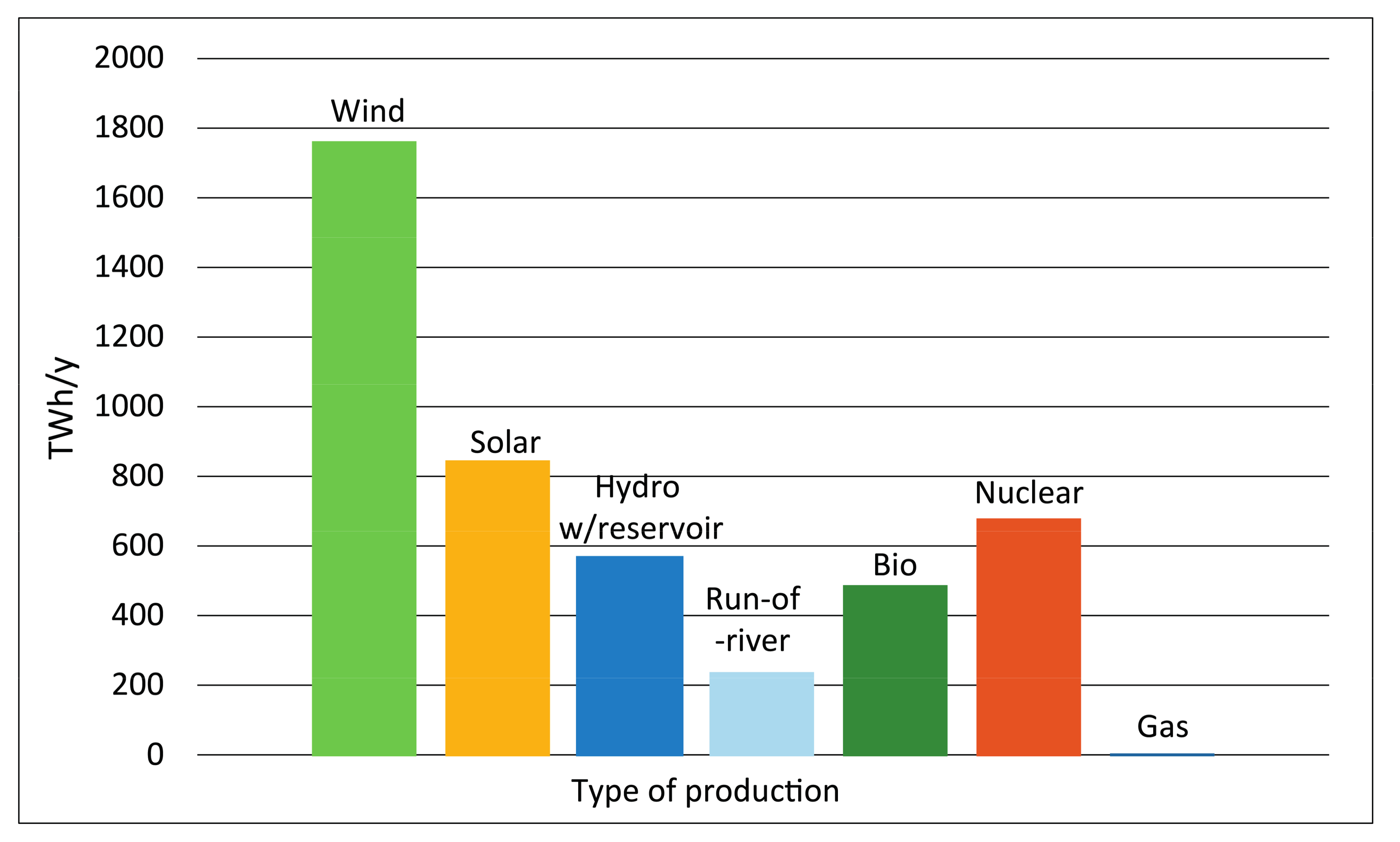
This study uses a scenario from the EU 7th Framework project eHighway2050. In eHighway2050, 28 research partners from the whole Europe (including among the European Network of Transmission System Operators for Electricity (ENTSO-E)) developed scenarios that aim to fulfil EU’s climate target and ambitions to 2050. The scenarios have high spatial resolution including several regions within each country. One of the scenarios, 100% RES (also called X-7), assumes large-scale deployment of both onshore and offshore wind and PV power production. Even though the scenario is called 100% RES, it includes gas for peak power production. Appendix A shows the assumptions for installed capacities in each region and in each country in Europe [17]. Appendix A also includes assumptions for demand per region. The assumption for the whole Europe is 4277 TWh/y. eHighway2050 does not show demand profiles per countries. Thus, this study uses present (2015) yearly profile per country from ENTSO-E [18]. The EMPS analysis of the 100% RES eHighway2050 scenario showed a system in large imbalances. In order to achieve a more realistic system, we added extra nuclear capacity to the system. The nuclear capacities and locations are from the X-5 eHighway2050 scenario. That extra capacity resulted in a lot of surplus in the analysis. Thus, we reduced the nuclear capacity with 40% in all regions compared to the X-5 scenario. Table A1 in Appendix A shows how the 95 GW extra nuclear capacity we added to the system is distributed on the nodes/regions in Figure 1. The assumed nuclear capacities in eHighway2050 reflect the long term political ambitions and targets in each country. E.g., there is no nuclear production in Germany. Figure 2 shows the aggregated production per year for Europe for the 100% RES scenario with nuclear added. Transmission capacities, marginal production costs per technology and costs for rationing (curtailment) of demand are also are from the eHighway2050 X-7 scenario, see Appendix A. Except for connection to other Nordic countries (Sweden, Denmark and Finland), Norway is presently only connected to the Netherland by 700 MW. Connections of 1400 MW between Norway and Germany and between Norway and UK are expected in a few years. As shown in Appendix A, eHighway2050 assumes great increases in transmission capacities towards 2050.
2.3. Modelling of Wind and Solar Power Production
Calculation of wind and photovoltaic (PV) power production is based on reanalysis data from 1948 to 2005. Wind speed and irradiation time series are from National Centers for Environmental Prediction (NCEP) data provided by NOAA/OAR/ESRL PSD, (Boulder, CO, USA) on their Web site [19]. The spatial resolution of the data is 2.5 degrees both in latitude and in longitude. The reference [20] describe the generation of hourly values and calculation of the power production from wind and radiation resources. The references also describe adjustment of the production in order to obtain reasonable capacity factors for the different geographical regions. Reference [21] describes validation of the model for hourly values. The model lacked adjustment for wind power production in Spain, Portugal, Italy, Czech Republic and countries in Southeast Europe. The simulated production for those countries where adjusted according to capacity factors from [22]. The offshore wind production in the North Sea was adjusted to a capacity factor of 40% in order to be in accordance with present results [23]. We used the reanalysis data and calculated hourly time series with wind and PV power production for all the 59 regions in Figure 1. In order to match the 75 years with hydrological data, the first 17 years with wind and radiation data were repeated twice.
2.4. Expansion of the Norwegian Hydropower System
Previous research identified possibilities for increased generation capacity in existing hydropower plants in Southwestern Norway. Reference [8] focused on the possibilities for increasing capacity with minimal environmental impact. No new or expanded reservoirs were assumed. Furthermore, present regulations regarding highest and lowest regulated water levels were also kept unchanged. Two possible cases for increases of capacities were identified, one case with 11.7 GW increased production capacity and 4.5 GW pumping capacity and another with 19 GW increased production capacity and 9.2 GW of pumping capacity. The power generation outputs in the two cases were mainly chosen such that the water level changes in the reservoirs did not exceed 13 cm/h at maximal production. According to research into the stranding of salmon in rivers, the water level should not sink by more than 13 cm/h [24]. Although this is not directly applicable to lakes, this was used as a rule of thumb for acceptable water level reductions in reservoirs.
Table 1 shows the possibilities for increases of production capacities and pumped storage that were identified in [8] for Southwestern Norway. The results are shown for individual plants in four regions. The column to the left shows the eHighway2050 scenario names (79_no etc.) of the EMPS nodes/regions (see Figure 1). In addition, it shows the names used in the Twenties project (SORLANDET etc.). In the following the names from the Twenties project is used. The rightmost column shows if the reservoir upstream to the plant is of type “Regulation” (R) or “Buffer” (B), (see Section 2.1). The increases of capacities were implemented in an initial version in the EMPS model in the EU project Twenties [25]. This study uses this implementation. The Twenties project primarily focused on the 11 GW version, and studied the utilization of the aggregated production capacity versus the increases of transmission capacities. The 75 years with hydrological data are SINTEF (Stiftelsen for INdustriell og Teknisk Forskning) Energy Research’s own data.
3. Results
This section presents results from the EMPS simulations of the X-7 eHighway2050 scenario. In the simulations, the optimal power dispatch is found for every 2-h (and 4-h in the weekends) time step. The simulations are sequentially run for the 75 years with stochastic input data. Three cases are defined. One case uses the present capacity in the Norwegian hydropower system (31 GW). The second case increases the capacity with 11.6 GW according to Table 1 and the third case increases the capacities with 19 GW. All other input data are equal for the three cases. In the relevant figures in the following sections results from the first case has red color, the second blue and the third green color. Section 3.1 presents impacts on water values from increases in hydropower production capacities, Section 3.2 impacts on reservoir operation, Section 3.3 production patterns and Section 3.4 power prices.
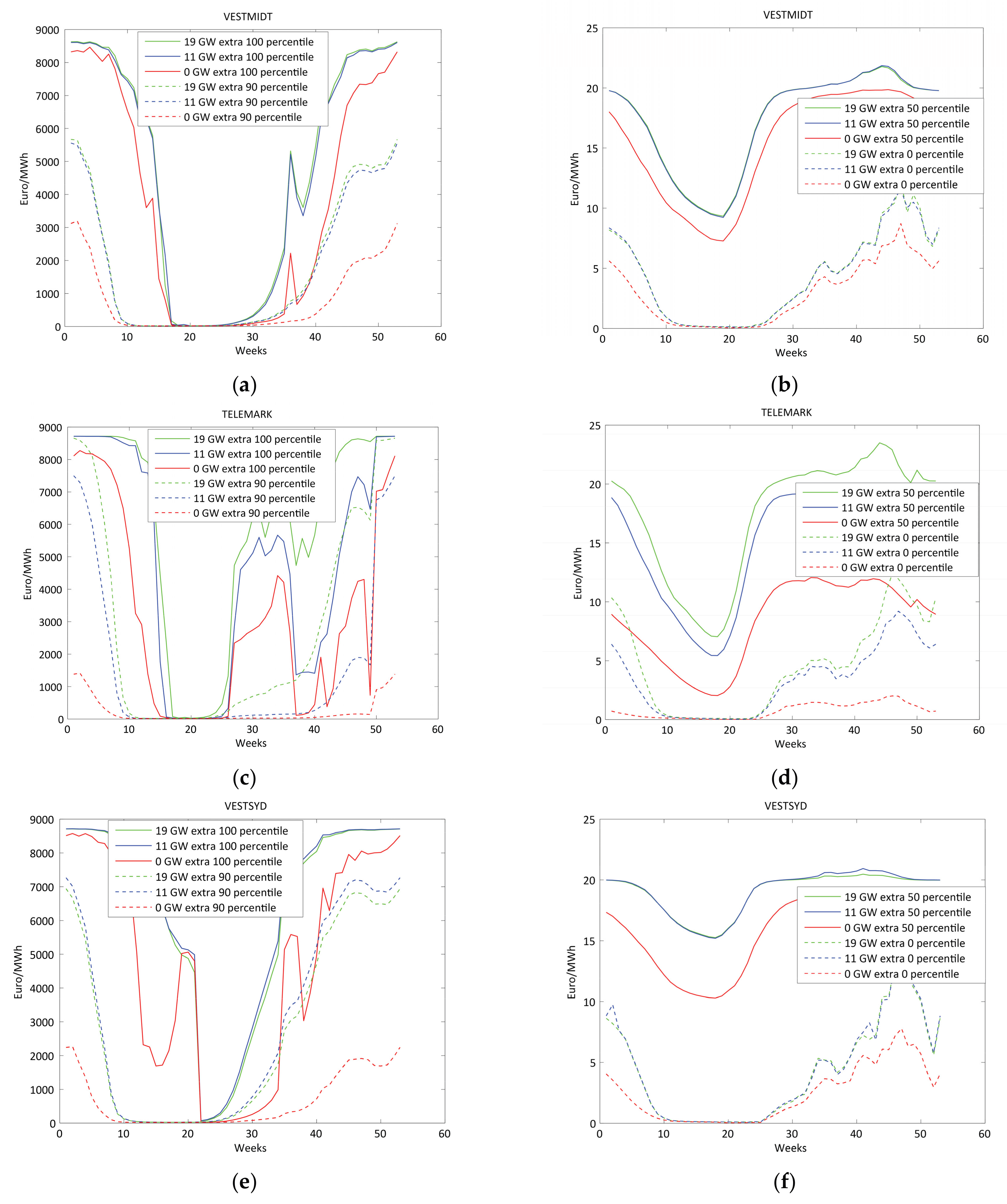
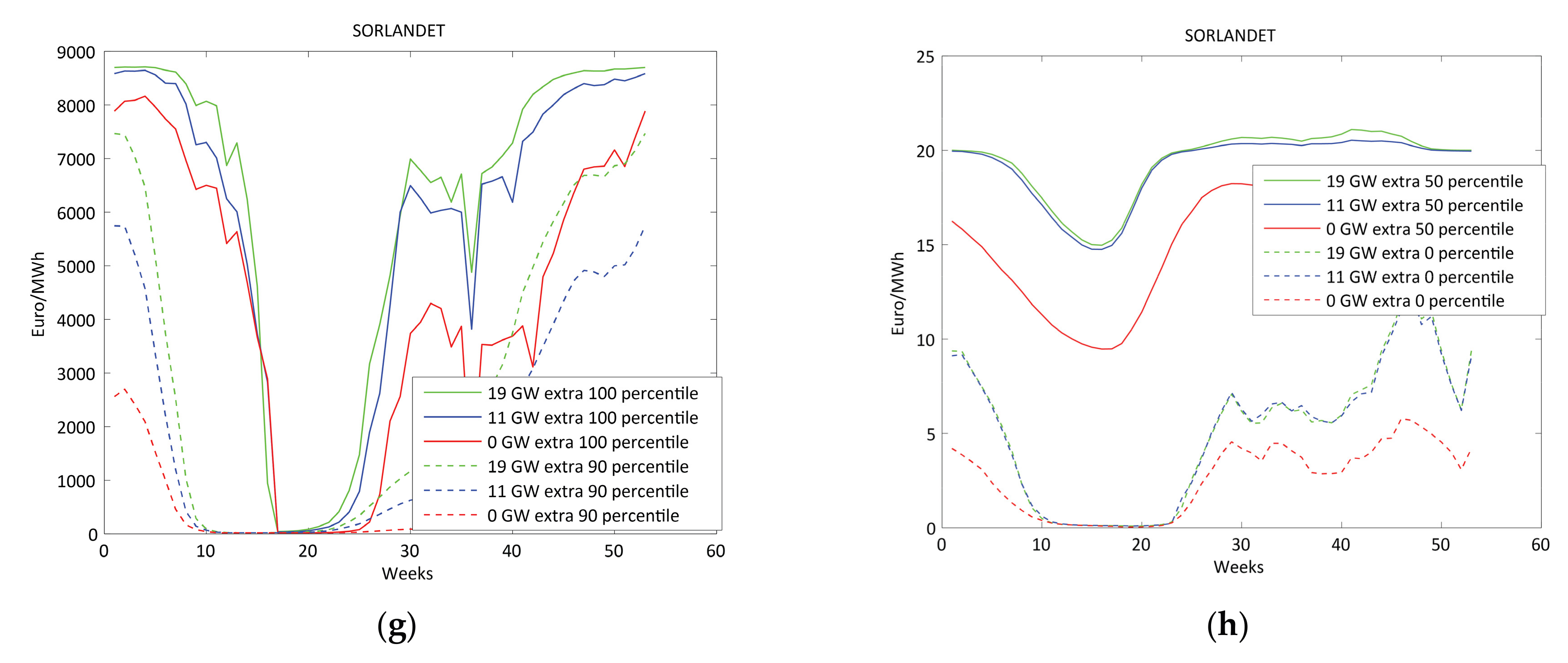
3.1. Water Values
Figure 3 shows percentiles for water values for the four regions in Norway with increases in hydropower production capacities. Some observations from Figure 3 are:
- Water vales are impacted by seasonal variation in weather and load. The water values are highest in the winter period because of low inflow/overflow risks and high demand. The water values are lowest in the early summer, i.e., in the snow melting season with high inflows and overflow risk.
- The highest water values are in some few situations close to the rationing price (10,000 Euro/MWh). Such situations will typically be caused by very dry years or with several dry years following each other. There will be limited water in the reservoirs and the water values will increase.
- The lowest water values are in most cases higher than 5–10 Euro/MWh. Non-flexible production (wind, PV, run-of-river and nuclear) have lower prices. Thus, the hydropower system will not produce when there is surplus in the non-flexible production. The lowest marginal prices for flexible plants are 10 Euro/MWh (see Appendix A).
- For all four regions, the water values increase with increases in generation capacity. Assuming the hydro producer is a price taker, increases in flexibility will result in increased water values because the hydropower plants can produce more when the prices are high. Furthermore, the risk for spillage decreases which also gives higher water values. However, we are analyzing large changes and the producer cannot be assumed to a price taker. Increased flexibility decreases price variation which again can give reduced water values depending on the producer’s flexibility. Plants with high flexibility will get lower water values with reduced price variation and the opposite might be the case for plants with little flexibility. The water value method in the EMPS model does not consider increases in pump capacity. It should be mentioned that the increased water values due to increased flexibility is not necessarily based on increased flexibility in the physical system. As described in Section 2.1, the EMPS model calculates the water values aggregated per region. In this study, the capacity increases are assumed to be on a few plants and reservoirs. In the physical system, there may be restrictions such that the increased capacity has limited effect, e.g., due to limitation in inflow, restrictions on depletion of reservoirs etc. Calculation of water values is complex, and it can be difficult to explain exactly why things are changing one or another way.
3.2. Reservoir Operation
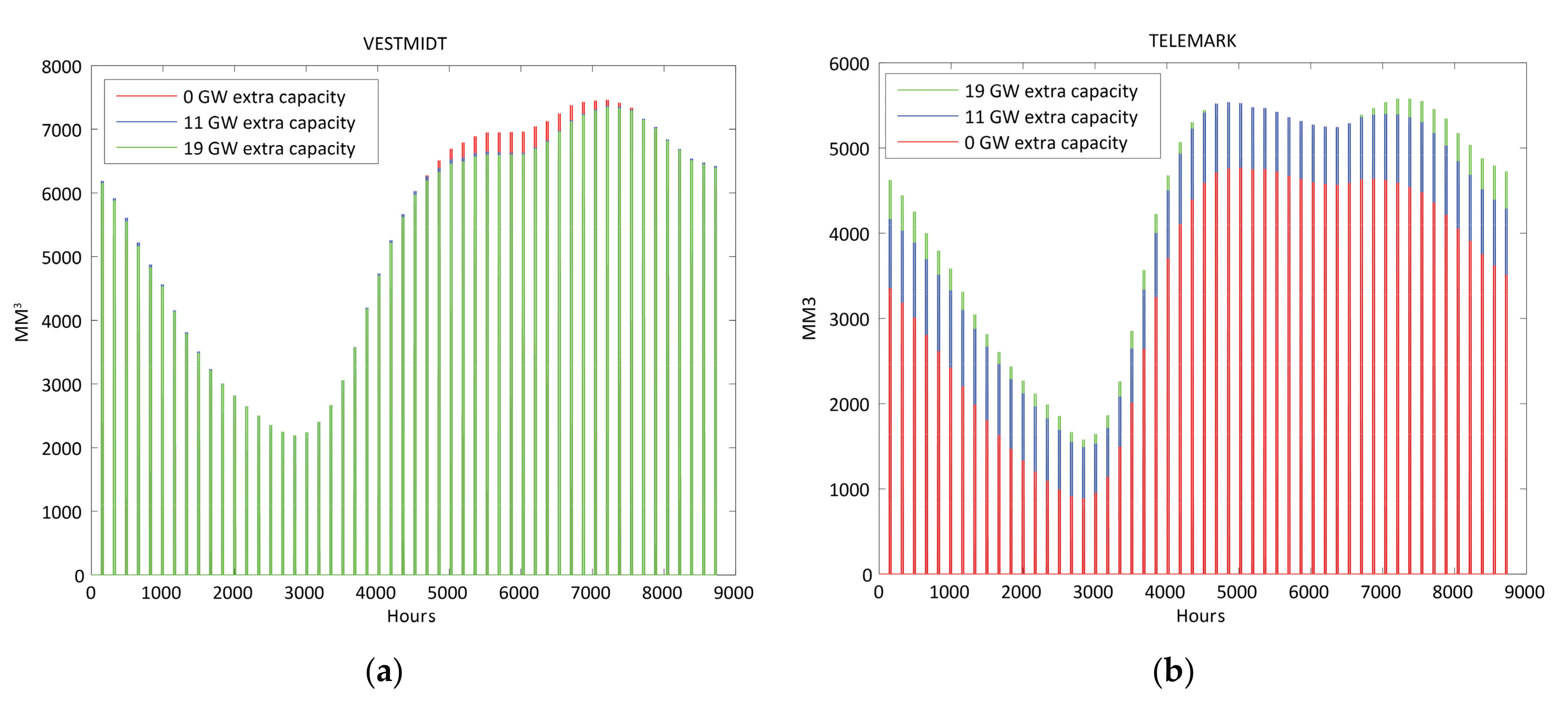
Figure 4 shows the yearly patterns for aggregated reservoir level for the four regions with increase in hydropower generation capacity. The patterns are the average results for 75 years with simulations. Most large reservoirs in Norway have a similar yearly shape of the reservoir levels. The reservoirs are depleted in the winter, until the snow melting period starts in the spring. They are filled up during spring, summer and autumn. Three regions, VESTSYD, SORLANDET and TELEMARK have higher average reservoir level with increased capacities while the fourth region, VESTMIDT have almost equal levels. The three regions with increased level also have increases in pump capacities (see Table 1) and that is probably the main reason for the increases. Water are pumped to higher reservoirs in the river system when the prices are very low. Many periods with pumping instead of producing reduce use of water, i.e., the reservoir level increases. VESTMIDT on the other hand, has no increases in pump capacity.
Since the water values increases for all four regions, there will be less situations where it is valuable to produce. Thus, in situations where it is profitable to produce with the present capacity and it is not profitable to produce with increased capacity, the level in the reservoirs increases. On the other hand, when it is valuable to produce, the plants produce more with the increased capacity and the reservoir level decreases more.
Kvilldal and Lysebotn are two reservoirs in the SORLANDET region (see Table 1). They are reservoirs upstream to plants with increased capacity.
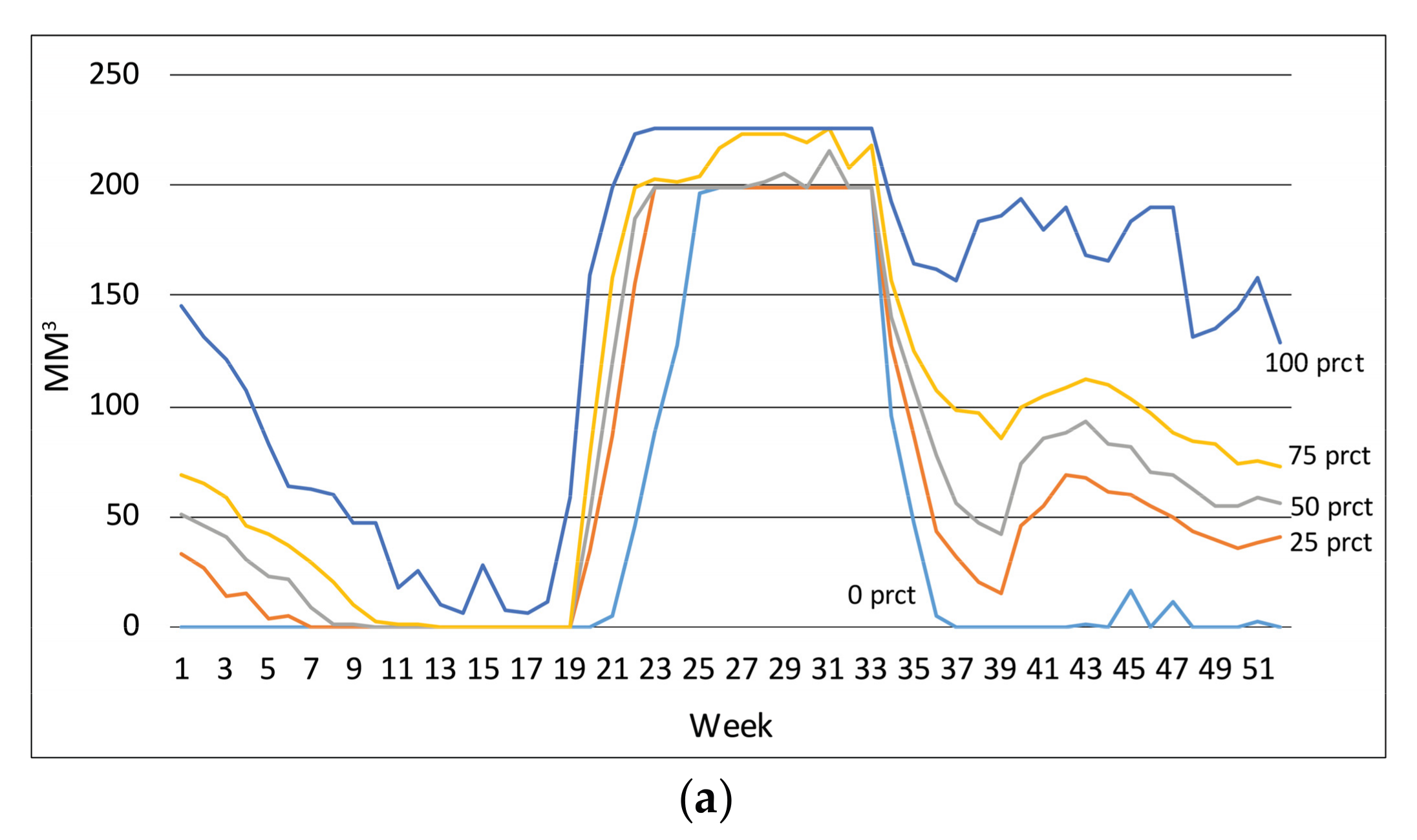
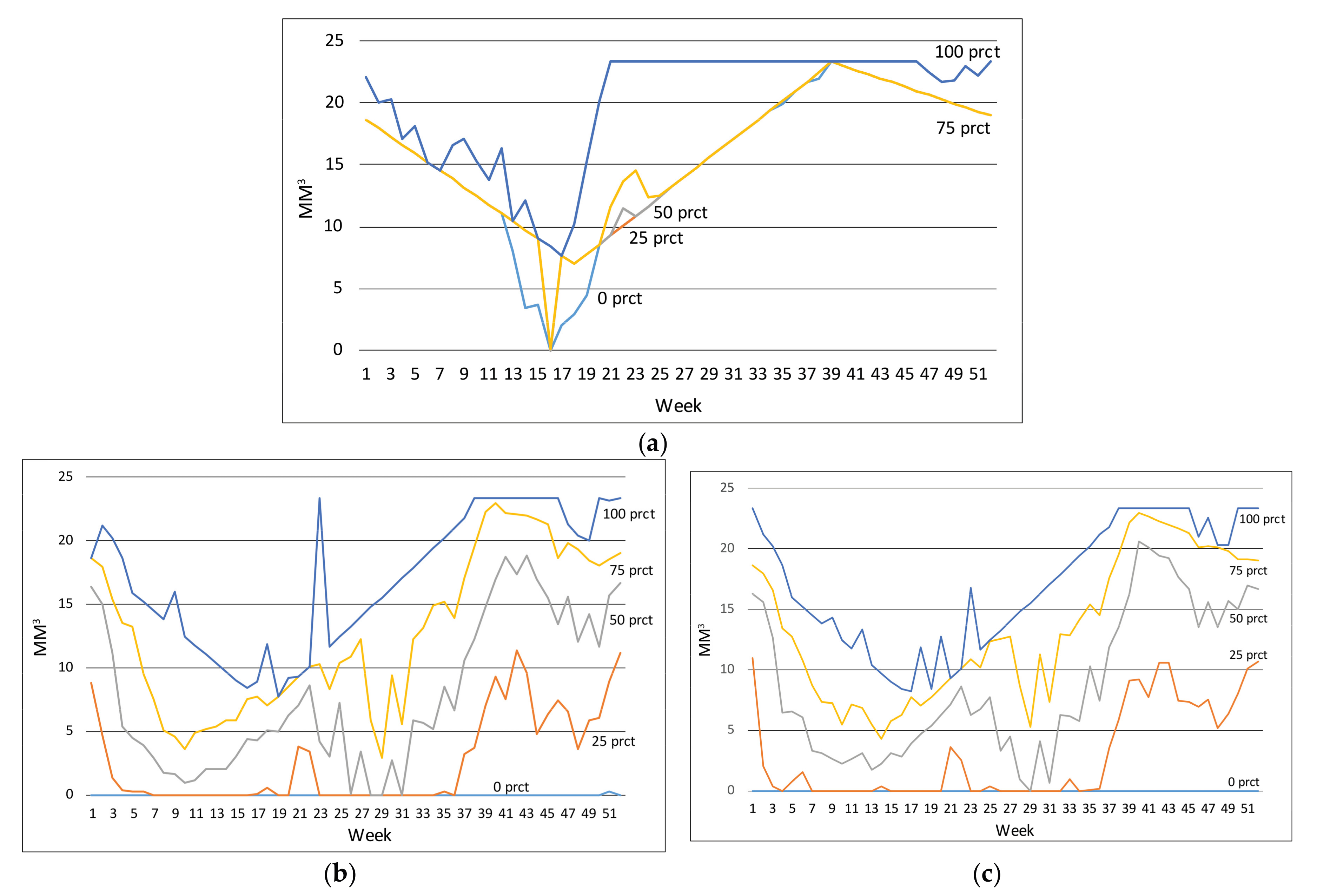
Figure 5 and Figure 6 show how the reservoir levels change over the year for those two reservoirs, when the hydropower generation capacity in Norway changes from present system to 11 GW and 19 GW extra capacity. The figures show percentiles (0, 25, 50, 75 and 100) of reservoir level for every time step over the year for 75 years with simulations. For example, for every time step in the 75 years with simulations, the reservoir level is above the 0-percentile. Furthermore, for every time step the reservoirs level is below the 100-percentile etc.
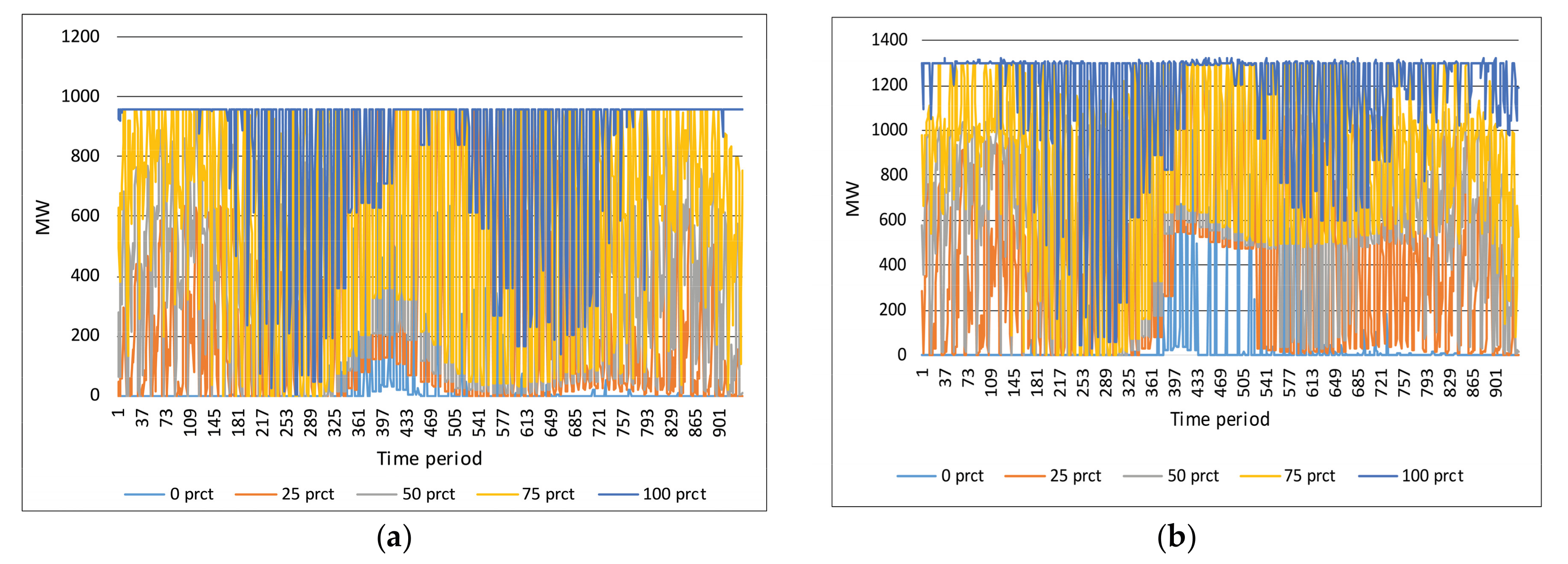
Figure 5 shows the percentiles for reservoir levels for Kvilldal, and Figure 6 shows the percentiles for Lysebotn reservoir. The two reservoirs have very different maximum storage capacity: Kvilldal 237 MM3 and Lysebotn 23.3 MM3. Kvilldal is a regulation reservoir, while Lysebotn is a buffer reservoir (see Section 2.1).
Figure 5 shows that for Kvilldal the reservoir level is to some degree higher in the autumn for the cases 11 GW and 19 GW extra capacity than for the case with the present capacity. One important reason is that it is pumped a lot to the reservoir in the summer period for the two cases with extra capacity. In the last weeks before the melting season starts, the reservoir may be nearly empty in all three cases. Expects for those weeks and the very dry years (the 0 percentile), there is water available in the reservoir such that production is possible.
As shown in Figure 6, the buffer reservoir upstream to Lysebotn is empty only in very few situations with the present hydropower capacity. It is one or a few weeks before the melting season starts (approximately week 17). After increase of capacities, the reservoir may be empty all weeks in the year (the 0 percentile). For 25% of the time steps, there are many weeks with empty reservoir. In particular, the reservoir is empty in the first half part of a year.
3.3. Production Pattern
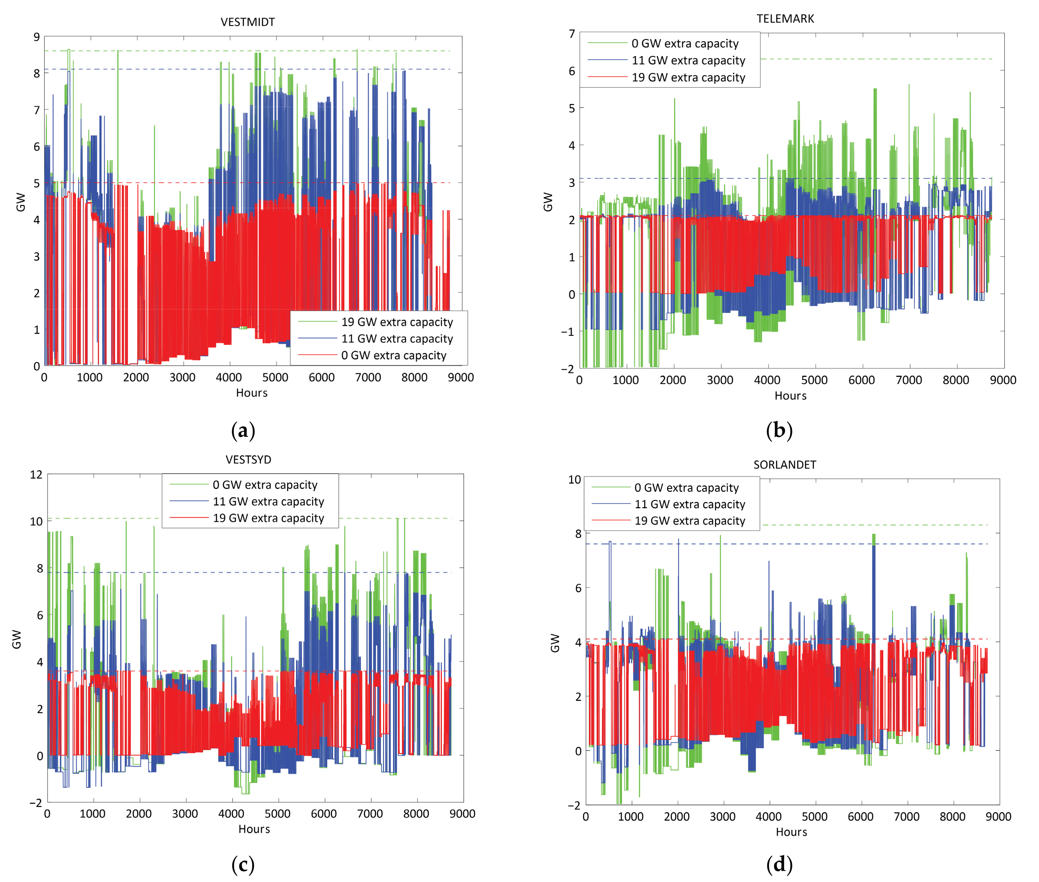
Figure 7 shows the aggregated hydropower production hour by hour for each of the four regions for year 38. Year 38 is selected since the power prices this year are close the average prices for the 75 years with simulations. The broken horizontal lines show the maximum available production capacities for the three different cases.
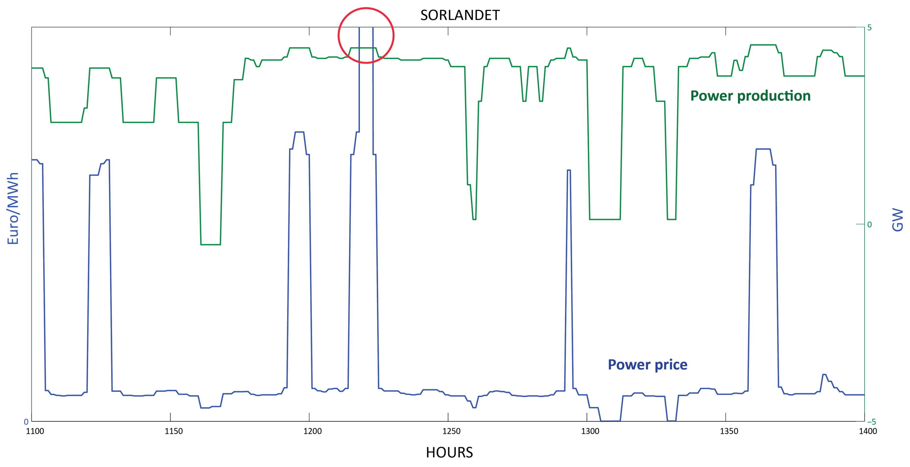
Figure 7 shows significant changes in production patterns for the three cases. However, the example year also indicates that the extra capacity is not fully utilized. For TELEMARK and for SORLANDET the extra maximum capacities of 6.3 GW and 8.3 GW, respectively, in the 19 GW case, are never used in the example year. For SORLANDET, there is limited use of the extra capacities the whole example year. For TELEMARK, VESTMIDT and VESTSYD the extra capacities are use more frequently in the second part of the year. Figure 8 shows the hydropower production in the region SORLANDET for the hours 1100 to 1400 in year 38 for the 11 GW extra capacity case. Figure 8 shows that in spite of rationing price around hour 1220 (marked with red circle), the hydropower plants are not producing at maximum capacity. Only less than 5 GW out of the installed 7.6 GW is producing. There are also several other hours with prices around 200 Euro/MWh and limited production on SORLANDET.
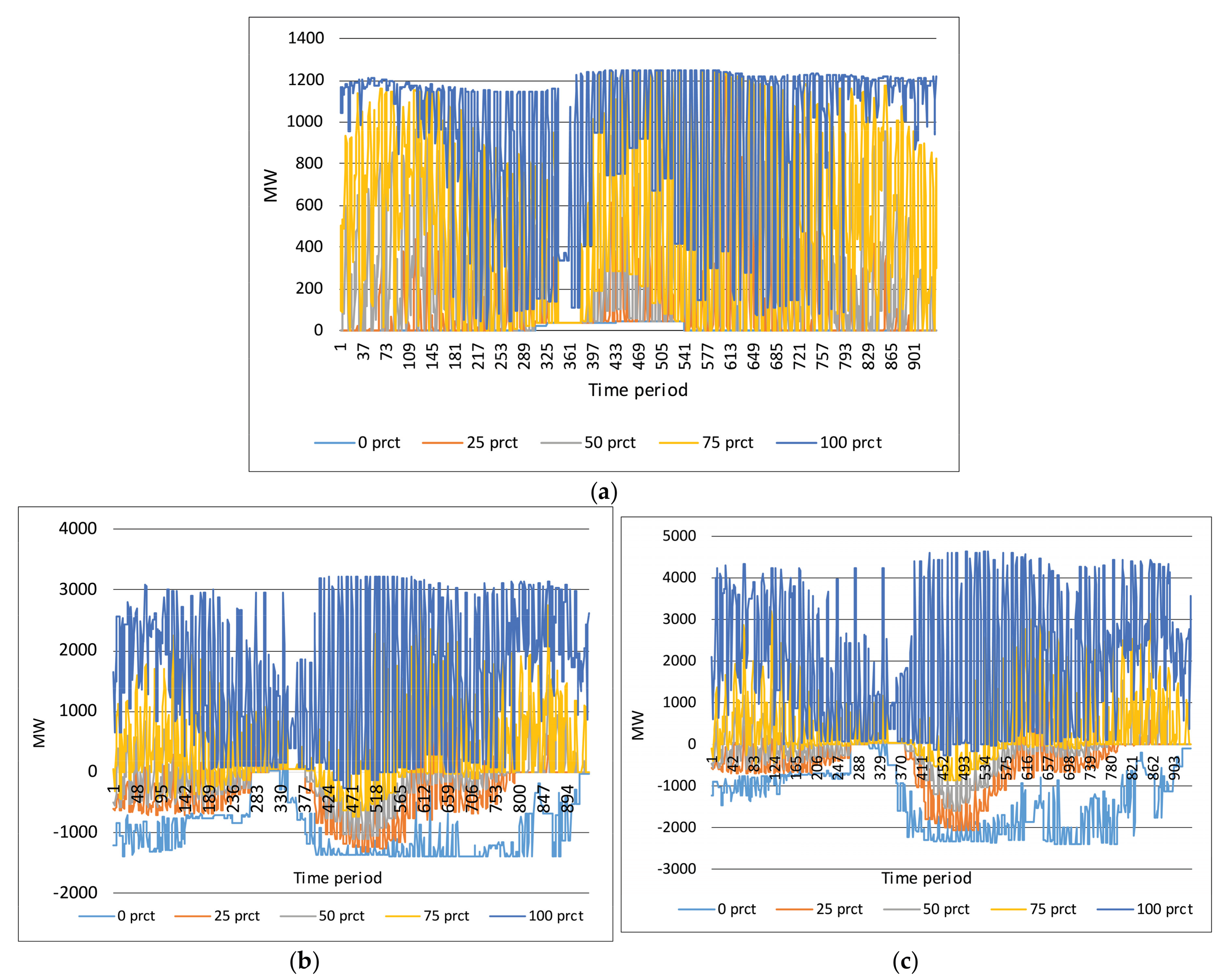
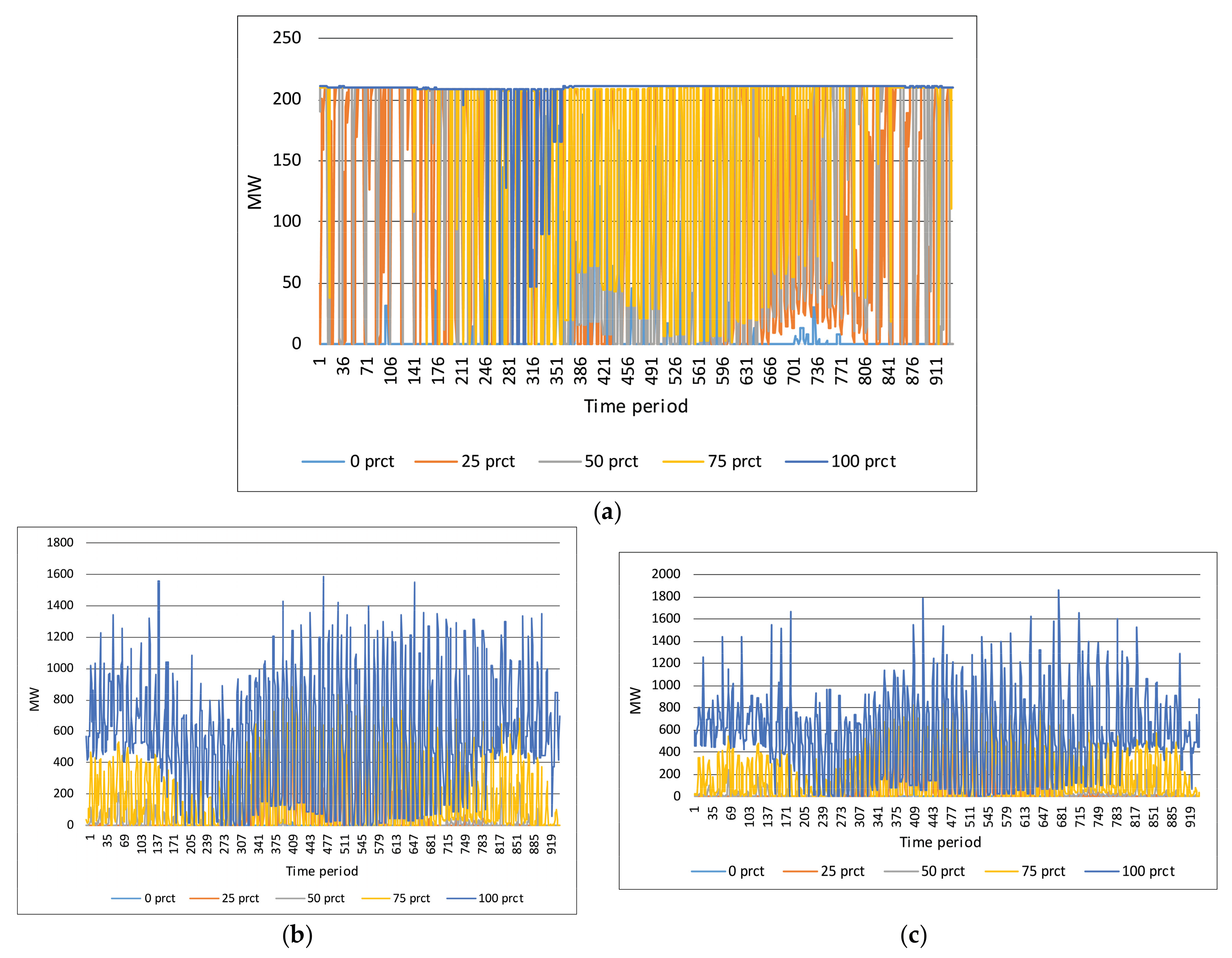
Reasons for the limited use of the capacities are discussed below. Before the discussion, the yearly production pattern for some single plants are discussed. Figure 9, Figure 10 and Figure 11 show the 0, 25, 50, 75 and 100 percentiles for the yearly power production in Kvilldal, Tonstad and Lysebotn, respectively, for the cases 0 GW, 11 GW and 19 GW (not Tonstad) extra capacity for 75 years with simulation. The unit on the x-axis for those figures is time period. There are 18 periods/week × 52 weeks = 936 periods each year. 18 periods/week is because every week day has a time resolution of 2 h and Saturday and Sunday have a resolution of 4 h. Each two-hour period is averaged in the presentation for the weekdays and correspondingly for the weekends. Thus, there are twelve 2-hour periods with average data for the week days and 6 for the weekends, i.e., 18 periods peer week.
Kvilldal is utilizing the new capacities fully. It produces at maximum in high price periods and pumps in low price periods and in the snow melting season. In the summer, it goes from production in many time periods in the present system (0 GW) to pumping based on increased pumping capacities. In the weeks before the filling season starts (approximately from time step 360), there is not enough water to produce at full capacity. The 100% percentile for the 11 GW and the 19 GW extra capacity is almost equal for those weeks and only ca. 1000 MW over the case without any extra capacity. The 75% percentile in the winter, is similar for all three cases. It is 500–1000 MW higher in the beginning and the end of the year for the 11 and the 19 GW case compared to the present case. For Kvilldal, the pump capacity is used for pumping in all time steps except for the weeks before the melting season starts. The pumping capacity is 1.4 GW in the 11 GW case and 2.4 GW in the 19 GW case. However, the pumping is almost equal for the two cases in the late winter period. There is probably too little water in the lower reservoirs to increase the pumping in the last part of the winter period.
As shown in Figure 10, Tonstad plant never uses its increased capacity. Only about 1.3 out of 2.1 GW is used. This is due to lack of water, mainly because of the small size of the upstream reservoir: 0.1 MM3. The maximum depletion of the Tonstad buffer reservoir is 555 m3/s, i.e., at maximum the depletion from the buffer reservoir is 2 MM3 each hour (555 × 3600/100,000 MM3). The inflow to the buffer reservoir is at maximum 170 m3/s, i.e., the buffer reservoir is filled up with ca. 1/3 speed of which it can be depleted.
Thus, there is not sufficient water in the reservoir such that Tonstad can produce at full capacity for an hour. If increases of generation capacities at Tonstad plant shall be efficient, the buffer reservoir and the inflow to the reservoir must be increased. Still, there may be other limitations in the river system.
Lysebotn increases production capacities from 0.2 GW to 1.6 (11 GW case) and further to 2.0 GW (19 GW case). However, it never fully uses its new capacities. The 100 percentile increases significantly, from 0.2 to ca. 1–1.2 GW, but never to its full potential. The main reason is the same as for Tonstad. The upstream reservoir is too small for the plant capacity. Furthermore, the EMPS model does not distribute water to buffer reservoirs such that the plant can produce at full capacity in high price periods. The buffer reservoirs are as explained in Section 2.1 depleted and filled according to their individual rule curve. This is visible in Figure 6 where the yellow curve in the present case (up to the right) is equal to the rule curve for this reservoir. Lysebotn reservoir is in most cases filled up and depleted according to this rule curve. For both cases with increased capacity, the 100-percentile (the blue curve) is for most time periods equal to the rule curve. i.e., the reservoir is in most weeks filled according to the rule curve and then depleted again due to production with high capacity. If the buffer reservoir had been filled up to its maximum, the Lysebotn plant could probably have produced more in many time periods.
As shown above, there are several reasons for the limited use of the capacities:
- Physical limitations within the water courses.New capacity is included in the cascade coupled river system by increasing the capacity of a few existing plants. The simulation results show that some of the increases cannot be utilized fully without further increases in other parts of the water course that limits the utilization of the new capacity.
- Model deficitsThe EMPS model uses aggregated water values in combination with a heuristic to find the optimal hydro schedule for a given week and weather scenario. This heuristic of the EMPS model is not a formal optimization that take into account optimally the consequences of sequential decisions for every plant in the serial water course. E.g. some plants should possibly produce maximum for all hours within the week, regardless of the market price, to make possible maximum production for one specific plant for a few peak hours. The heuristic gives a valid solution that is not necessary optimal for a serial water course with many time periods within the week. Furthermore, all reservoirs and plants should be included in an optimization procedure. As explained above, filling and depletion of buffer reservoirs according to individual curves, limits utilisation of the increased capacity.
- Limited transmission capacity.There are very high transmission capacities in the eHighway2050 scenario (see Table 1) and power prices are almost equal in several regions. If there is deficit of capacity in an adjacent region and lack of transmission capacities to the region, the hydropower capacity may not be fully utilized. An inspection of the utilization of connectors reveals that for a few hours there are limitation in capacities.
3.4. Prices
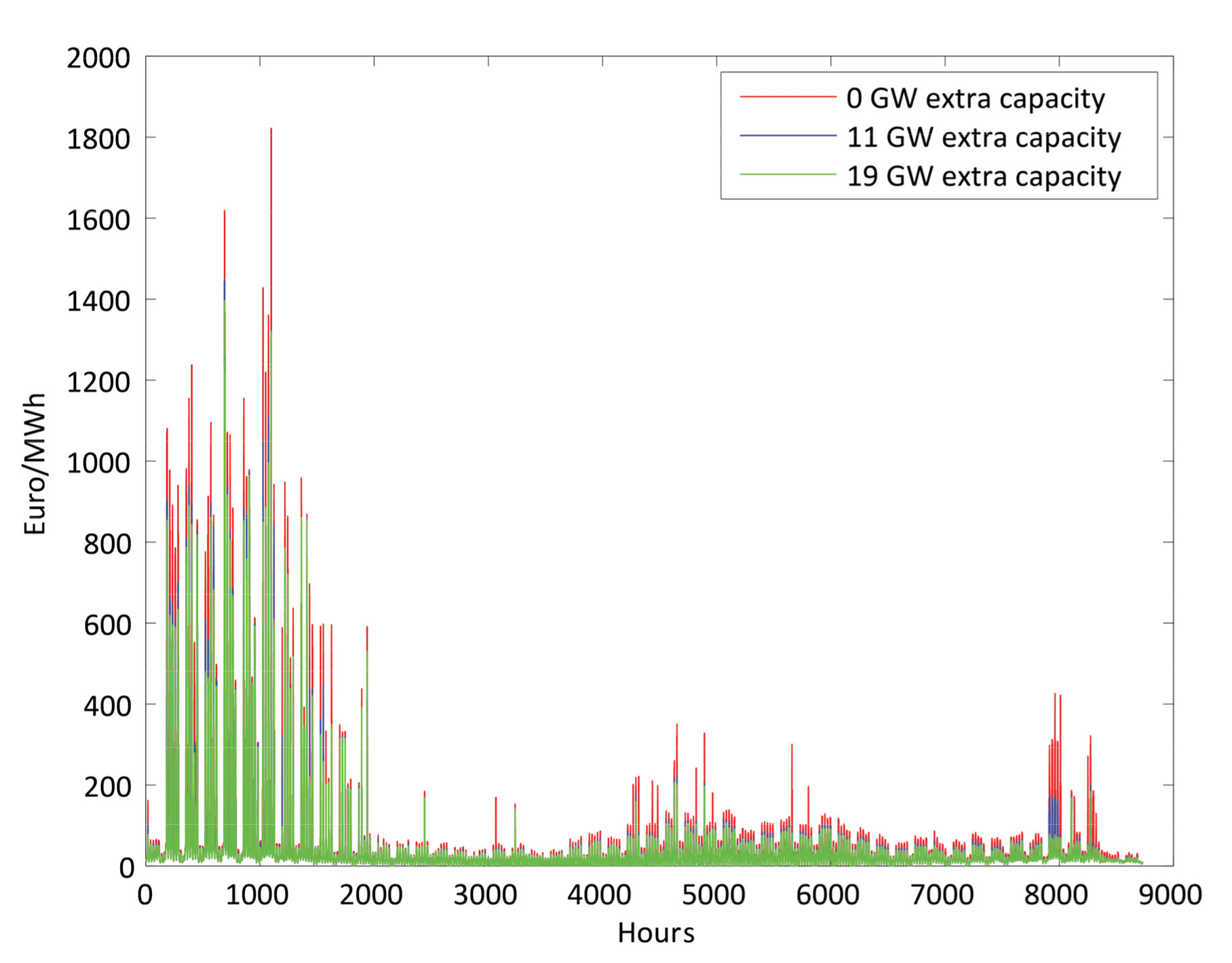
Reference [15] shows that the average power prices for Germany, the Netherlands, UK and France were reduced with up to 20% with increased generation capacities in the Norwegian hydropower system of up to 19 GW. The price reduction is case sensitive. Large transmission capacities between countries are assumed (from eHighway2050). The large capacities result in complete vanishing of bottlenecks and almost equal prices in e.g., southern Norway and in UK, the Netherlands and Germany. Figure 12 shows power prices at SORLANDET hour by hour averaged over 75 years with stochastic climatic input data.
The figure shows that the prices are highest for the case with the present capacity in the Norwegian hydropower system, lower for the case with 11 GW extra capacity and lowest for the case with 19 GW extra capacity. The prices are 0–50 Euro/MWh a main part of the year. In the beginning of the year, there may be periods with rationing prices. Due to the large transmission capacities, there are rationing prices in many regions when there is curtailment of demand in one single region. Averaged over 75 years with simulations the result is periods with prices up to ca. 1500 Euro/MWh. SORLANDET never has rationing itself, but adjacent regions like the Netherlands, north of Germany and UK have short periods where demand is curtailed (see Appendix B). In average over 75 years, SORLANDET has periods with prices above 300 Euro/MWh 22 h per year. The total rationing in Europe averaged over 75 years is ca. 0.2 TWh/y. The average high prices are concentrated to the first 2000 h of the year, except for a few periods at the end of the year. One reason for fewer periods in the end than in the beginning of the year, is that the consumption is lower in the two last weeks of the year than it is in January and February. Lower production in the Norwegian hydropower system (see Figure 7) due to limited water in the reservoirs probably also contribute to the periods with high prices.
4. Discussion and Findings
This paper aims to show the impacts on the Norwegian hydropower system in a scenario where it operates as a “battery” for future variable wind and solar power production in Europe. The study analyses increased capacity in the Norwegian hydropower production of 11.7 and 19 GW in addition to the present capacity of ca. 31 GW. Ongoing studies indicate that for the same scenario as used in this study, increases in the Norwegian hydropower generation capacity significantly reduces the prices in neighbouring countries [15].
This analysis uses a very detailed representation of the Norwegian hydropower system. For the scenarios analyzed, the water values increase, the reservoir levels increase for three out of four regions included in the study and there is a significant change in average production pattern over the year with increased capacity in the Norwegian hydropower system. For many time periods the power production increases when the prices are high (higher than the water values). Furthermore, the system pumps from lower to higher reservoirs in situations with very low prices and also related to seasonal inflow. This is how the system should work. Maximizing the production in high price periods increase the producer’s income. Pumping in low price periods increases the flexibility for the high price periods. However, the study also shows that there are many time periods with prices much higher than the water values, and with no or limited increases in utilization of available hydropower capacity. One reason is small buffer reservoir upstream to the plant with increased capacity. The reservoirs are so small that they are depleted within a short time period and there is not enough available capacity or water upstream. Another reason is the way the EMPS model works:
- The EMPS model calculate water values and target reservoirs per week. High price variations within a week will not be reflected in the water value.
- In the reservoir drawdown procedure, the main objective in the filling season is to avoid spillage and in the depletion season to avoid capacity deficit and to minimize spillage in the coming spring inflow period. The EMPS model does not optimize depletion of the water over the week, in such a way that plants with increased capacity have available water to produce extra in time periods with high prices.
- Buffer reservoirs are not included in the reservoir drawdown strategy and when energy is distributed within each region/node, the buffer reservoirs are only filled and depleted according to a management curve per reservoir and not related to the available energy in the river system.
Based on the findings in this study, further research should do an in-depth study of where it is optimal to allocate new production capacities and pumps. This study shows an example of a large increase of capacity that seems efficient: Kvilldal with large reservoirs both upstream and downstream. It also shows examples of less efficient implementations like Tonstad and Lysebotn. The production in those plants are limited by their small upstream buffer reservoirs. Future studies should both investigate how increases of capacities can be utilized for each plant with their upstream and downstream reservoirs as well as how all the plants interact together in the total cascade coupled river system. For some of the rivers systems e.g., in TELEMARK, it may not be efficient at all to do one large increase of capacity. This is due to many small reservoirs in the river system. Those small reservoirs may limit the utilization of the new capacity even though the increase is implemented on a plant with a large reservoir. Several smaller increases could be considered.
Further research should also use a model which optimizes of the water level in every reservoir and in every time step. The prototype model SOVN (Stochastic Optimization model with individual water values and net restrictions) is a candidate for such studies [26]. This study uses one scenario for the future European power system. Further research should analyze how increases in Norwegian hydropower capacity impact several different scenarios. Sensitivity related to yearly demand in the Nordic region should be included. The present study mainly uses input data from the eHighway2050 project. The demand in Norway and Sweden is reduced compared to present level, while some relevant studies expect increase. E.g. Reference [27] expects that the demand increases with 50 TWh/y in the whole Nordic region including 15 TWh/y in Norway from today and to 2040. However, Reference [15] shows that the increases in the Norwegian hydropower generation capacity may significantly reduce future European power prices even with power demand at present level.
Transmission capacities are not studied in detail in this analysis. The study used assumptions from eHighway2050. Observations from the research indicate that some reduction of transmission capacities in Norway and between Norway and other countries are possible.
The strength of this study is the detailed representation of the Norwegian hydropower where every plant and every reservoir are separately modelled with their restrictions and regulations related to depletion limitation and to maximum and minimum reservoir level. Another strength is the 75 years with stochastic weather data. A weakness is the simplified modelling of thermal production. Both bio and gas plants are regulated up and down with no restrictions regarding start and stop cost and minimum production. Furthermore, requirements for rotating reserves are not included and is recommended for further studies. Finally, climate change may change the “framework” for the hydropower system with more precipitation, shorter season with frozen reservoirs and less need for saving water to the melting season. The changes will probably increase the flexibility of the hydropower system, but this is also recommended for further studies.
A question is if the use of Norwegian hydropower as a battery for balancing variable wind and PV power production in neighboring countries can be applied in other parts of the world? The report [28] mentions in their “Outlook” Section that countries with abundant hydropower resources use their reservoirs as “batteries” to balance variable generation in neighboring countries. The report mentions two examples. The first is the Canadian province of Manitoba and their large hydro-based system that is strongly interconnected with the grids of the US mid-west. As such, Manitoba Hydro can utilize their reservoirs to balance the output of major windfarm to the south. The second example in the report is Denmark using Norwegian hydropower to back up its wind and thermal grid. The report also writes that there is a large unused global potential of hydropower. Estimates indicate the availability of approximately 10,000 TWh/y. The report says that “how much of that will be developed is a matter of market conditions, government policy and the emergence of other competing renewable options such as solar PV, wind and biomass.” Our studies about Norwegian hydropower versus European future wind and PV power production, indicates that hydro, wind and solar should not be regarded only as competing, but more as complementary resources that all are needed to create a secure power supply without green-house-gas emissions. However, our study shows that for cascade coupled river systems with many reservoirs, detailed modelling and analysis of complex hydropower systems are needed.
Acknowledgments
The research is a part of the Norwegian project “Cedren HydroBalanace”. The authors thank the Norwegian Research Council and project partners for the financial support to the project.
Author Contributions
Ingeborg Graabak conducted a main part of the research work as a part of her PhD studies. She is the main author of this paper. Magnus Korpås is her supervisor and contributed with frequent discussion and recommendations related to the structure of the work. Both Stefan Jaehnertand and Birger Mo are EMPS experts and have been advisors related to the modelling work and to interpretations of the results.
Conflicts of Interest
The authors declare no conflict of interest.
Abbreviations
Abbreviation for other countries than UK, are mentioned in Appendix A.
| CSP | Concentrated Solar Power |
| EMPS | EFI’s (former name of SINTEF Energy Research) Multi-area power Market Simulator |
| ENTSO-E | The European Network of Transmission System Operators for Electricity |
| EU | European Union |
| MM3 | million cubic meters |
| PV | Photovoltaic |
| RES | Renewable Energy Sources |
| SOVN | Stochastic Optimization model with individual water values and net restrictions |
| TSO | Transmission System Operator |
| UK | United Kingdom |
Appendix A. Input Data to the EMPS Analysis
This paper uses the following abbreviations: au—Austria, be-Belgium, ch-Switzerland, cz—the Czech Republic, de—Germany, dk—Denmark, ee—Baltics, es—Spain*, fi—Finland, fr—France, lu—Luxembourg, ie—Ireland, it—Italy, nl—the Netherlands, no—Norway, ns—North-Sea, pl—Poland, ro—Romania* se—Sweden, si—Slovenia, uk—United Kingdom*. The node 04_es includes both Spain and Portugal. The node 59_ro includes Romania, Bulgaria, Hungary, Albania, Greece, Croatia, Montenegro, Former Yugoslav Republic of Macedonia, Serbia, Bosnia and Herzegovina and Slovakia. The node 73_ee includes Latvia. Lithuania and Estonia.
Figure 1 shows location of the nodes used in the following tables.

Table A1.
Installed capacities and demand per node/region (see Figure 1) (from eHighway2050).
Table A1.
Installed capacities and demand per node/region (see Figure 1) (from eHighway2050).
| Node/Region | Wind (GW) | Solar (GW) | Biomass I (GW) | Biomass II (GW) | OCGT (GW) | Nuclear (GW) | RoR (TWh/y) | Hydro with Reservoir (GW) | Max Reservoir (TWh) | Demand (TWh/y) |
|---|---|---|---|---|---|---|---|---|---|---|
| 04_es *) | 81 | 130 | 5 | 15 | 9 | 5 | 53 | 43 | 30 | 569 |
| 52_it | 41 | 116 | 4 | 15 | 9 | 0 | 26 | 22 | 26 | 431 |
| 25_fr | 124 | 114 | 8 | 21 | 16 | 43 | 57 | 32 | 10 | 649 |
| 28_be | 11 | 24 | 1 | 4 | 3 | 0 | 2 | 2 | 0 | 121 |
| 29_lu | 1 | 1 | 0 | 0 | 0 | 0 | 1 | 2 | 0 | 7 |
| 30_nl | 15 | 22 | 1 | 4 | 3 | 1 | 1 | 0 | 0 | 161 |
| 31_de | 32 | 15 | 1 | 3 | 2 | 0 | 1 | 1 | 0 | 111 |
| 32_de | 26 | 10 | 1 | 4 | 3 | 0 | 0 | 0 | 0 | 63 |
| 33_de | 12 | 11 | 1 | 2 | 4 | 0 | 1 | 1 | 0 | 145 |
| 34_de | 15 | 14 | 1 | 3 | 1 | 0 | 0 | 4 | 0 | 63 |
| 35_de | 7 | 11 | 1 | 3 | 1 | 0 | 0 | 1 | 0 | 90 |
| 36_de | 2 | 11 | 1 | 2 | 1 | 0 | 5 | 4 | 0 | 88 |
| 37_de | 4 | 26 | 1 | 4 | 2 | 0 | 17 | 1 | 0 | 105 |
| 38_dk | 14 | 1 | 1 | 2 | 1 | 0 | 0 | 0 | 0 | 23 |
| 72_dk | 5 | 1 | 0 | 1 | 1 | 0 | 0 | 0 | 0 | 19 |
| 39_cz | 10 | 13 | 1 | 4 | 2 | 7 | 2 | 3 | 1 | 72 |
| 45_pl | 82 | 24 | 4 | 11 | 3 | 6 | 12 | 4 | 1 | 172 |
| 47_ch | 1 | 15 | 0 | 1 | 2 | 0 | 20 | 14 | 1 | 77 |
| 49_at | 7 | 12 | 1 | 2 | 2 | 0 | 44 | 16 | 3 | 85 |
| 74_fi | 6 | 1 | 1 | 1 | 0 | 0 | 3 | 1 | 5 | 8 |
| 75_fi | 23 | 4 | 1 | 3 | 1 | 2 | 6 | 1 | 0 | 74 |
| 90_uk | 19 | 19 | 1 | 4 | 2 | 3 | 0 | 0 | 0 | 162 |
| 91_uk | 14 | 9 | 0 | 1 | 1 | 5 | 0 | 0 | 0 | 40 |
| 92_uk | 28 | 20 | 1 | 3 | 2 | 2 | 3 | 6 | 0 | 158 |
| 93_uk | 12 | 8 | 1 | 1 | 0 | 5 | 0 | 0 | 0 | 44 |
| 94_uk | 14 | 3 | 0 | 1 | 1 | 1 | 2 | 5 | 4 | 22 |
| 95_uk | 6 | 1 | 0 | 0 | 1 | 0 | 0 | 0 | 0 | 13 |
| 96_ie | 14 | 4 | 0 | 0 | 2 | 0 | 1 | 2 | 0 | 43 |
| 79_no | 1 | 1 | 0 | 0 | 0 | 0 | 0 | 5 | 12 | 6 |
| 7981_no | 1 | 0 | 0 | 0 | 0 | 0 | 0 | 4 | 13 | 12 |
| 80_no | 1 | 1 | 0 | 0 | 0 | 0 | 0 | 0 | 0 | 9 |
| 8081_no | 1 | 0 | 0 | 0 | 0 | 0 | 0 | 2 | 8 | 3 |
| 81_no | 1 | 0 | 0 | 0 | 0 | 0 | 0 | 5 | 12 | 12 |
| 82_no | 2 | 2 | 0 | 0 | 0 | 0 | 0 | 2 | 3 | 29 |
| 8082_no | 1 | 0 | 0 | 0 | 0 | 0 | 0 | 3 | 8 | 1 |
| 83_no | 2 | 1 | 0 | 0 | 0 | 0 | 0 | 3 | 9 | 17 |
| 84a_no | 1 | 0 | 0 | 0 | 0 | 0 | 0 | 2 | 11 | 4 |
| 84b_no | 1 | 0 | 0 | 0 | 0 | 0 | 0 | 2 | 8 | 7 |
| 85_no | 1 | 0 | 0 | 0 | 0 | 0 | 0 | 0 | 1 | 2 |
| 86a_se | 2 | 1 | 0 | 0 | 0 | 0 | 0 | 4 | 12 | 2 |
| 86b_se | 2 | 1 | 0 | 1 | 0 | 0 | 0 | 3 | 7 | 2 |
| 87a_se | 3 | 1 | 1 | 1 | 0 | 0 | 0 | 3 | 5 | 6 |
| 87b_se | 3 | 1 | 1 | 1 | 0 | 0 | 0 | 2 | 5 | 6 |
| 88_se | 11 | 4 | 1 | 1 | 0 | 3 | 0 | 2 | 3 | 89 |
| 89_se | 3 | 1 | 0 | 0 | 0 | 1 | 0 | 2 | 2 | 26 |
| 73_ee *) | 37 | 3 | 1 | 3 | 1 | 1 | 6 | 3 | 0 | 62 |
| 57_si | 0 | 2 | 0 | 1 | 0 | 1 | 9 | 0 | 0 | 15 |
| 59_ro *) | 59 | 70 | 9 | 20 | 1 | 10 | 94 | 44 | 8 | 349 |
| 106_ns | 22 | 0 | 0 | 0 | 0 | 0 | 0 | 0 | 0 | 0 |
| 107_ns | 11 | 0 | 0 | 0 | 0 | 0 | 0 | 0 | 0 | 0 |
| 108_ns | 2 | 0 | 0 | 0 | 0 | 0 | 0 | 0 | 0 | 0 |
| 109_ns | 2 | 0 | 0 | 0 | 0 | 0 | 0 | 0 | 0 | 0 |
| 110_ns | 16 | 0 | 0 | 0 | 0 | 0 | 0 | 0 | 0 | 0 |
| 111_ns | 27 | 0 | 0 | 0 | 0 | 0 | 0 | 0 | 0 | 0 |
| 112_ns | 19 | 0 | 0 | 0 | 0 | 0 | 0 | 0 | 0 | 0 |
| 113_ns | 6 | 0 | 0 | 0 | 0 | 0 | 0 | 0 | 0 | 0 |
| 114_ns | 3 | 0 | 0 | 0 | 0 | 0 | 0 | 0 | 0 | 0 |
| 115_ns | 3 | 0 | 0 | 0 | 0 | 0 | 0 | 0 | 0 | 0 |
| 116_ns | 3 | 0 | 0 | 0 | 0 | 0 | 0 | 0 | 0 | 0 |
| TOTAL | 875 | 732 | 50 | 140 | 73 | 95 | 365 | 256 | 207 | 4277 |
eHighway2050 assumes both PV and Concentrated Solar Production (CSP). All solar power production is modelled as PV in this study. Furthermore, eHighway2050 assumes import of solar power production from North Africa to Europe. This is modelled as extra PV power production in South European countries in our study. Run-of-river for Norway and Sweden are included in Hydropower with reservoirs.
Table A2.
Transmission capacities (see Figure 1) (from eHighway2050 X-7 scenario).
Table A2.
Transmission capacities (see Figure 1) (from eHighway2050 X-7 scenario).
| To-from | [MW] | To-from | [MW] | To-from | [MW] |
|---|---|---|---|---|---|
| 04_es-25_fr | 16,900 | 36_de-47_ch | 6000 | 8082_no-81_no | 7000 |
| 52_it-25_fr | 5800 | 36_de-49_at | 2800 | 80_no-82_no | 6300 |
| 25_fr-47_ch | 9500 | 37_de-39_cz | 2000 | 81_no-83_no | 1095 |
| 25_fr-96_ie | 5700 | 37_de-49_at | 16,000 | 82_no-83_no | 1100 |
| 25_fr-90_uk | 15,000 | 38_dk-72_dk | 600 | 82_no-88_se | 2148 |
| 25_fr-28_be | 7600 | 38_dk-79_no | 1700 | 83_no-84a_no | 1900 |
| 25_fr-35_de | 7100 | 38_dk-88_se | 740 | 84a_no-84b_no | 1100 |
| 25_fr-36_de | 1800 | 39_cz-45_pl | 4100 | 83_no-87b_se | 1000 |
| 28_be-29_lu | 700 | 39_cz-59_ro | 2700 | 84b_no-86a_se | 700 |
| 28_be-30_nl | 13,500 | 39_cz-49_at | 2100 | 84a_no-87a_se | 250 |
| 28_be-33_de | 6000 | 45_pl-73_ee | 9000 | 86a_se-86b_se | 8200 |
| 28_be-90_uk | 5000 | 45_pl-59_ro | 600 | 86b_se-87b_se | 8200 |
| 29_lu-35_de | 2900 | 47_ch-49_at | 2400 | 87a_se-87b_se | 16,300 |
| 30_nl-31_de | 1400 | 47_ch-52_it | 8500 | 87b_se-88_se | 16,300 |
| 30_nl-33_de | 7100 | 49_at-52_it | 10,300 | 88_se-89_se | 13,500 |
| 30_nl-38_dk | 700 | 49_at-57_si | 1600 | 89_se-45_pl | 600 |
| 30_nl-79_no | 14,700 | 49_at-59_ro | 1600 | 85_no-84b_no | 9500 |
| 30_nl-90_uk | 1000 | 52_it-57_si | 3600 | 73_ee-75_fi | 5000 |
| 31_de-32_de | 6400 | 72_dk-89_se | 1700 | 57_si-59_ro | 4300 |
| 31_de-33_de | 17,330 | 74_fi-75_fi | 3500 | 73_ee-88_se | 700 |
| 31_de-35_de | 6300 | 74_fi-85_no | 50 | 59_ro-52_it | 15,000 |
| 31_de-36_de | 7000 | 74_fi-86b_se | 1800 | 106_ns-90_uk | 100,000 |
| 31_de-37_de | 4000 | 75_fi-88_se | 1350 | 107_ns-92_uk | 100,000 |
| 31_de-38_dk | 3000 | 90_uk-91_uk | 7600 | 108_ns-93_uk | 100,000 |
| 31_de-79_no | 10,400 | 91_uk-92_uk | 5000 | 109_ns-94_uk | 100,000 |
| 31_de-89_se | 5200 | 92_uk-90_uk | 13,000 | 110_ns-28_be | 100,000 |
| 31_de-34_de | 9300 | 93_uk-92_uk | 11,900 | 111_ns-30_nl | 100,000 |
| 32_de-45_pl | 3400 | 92_uk-96_ie | 2500 | 112_ns-113_ns | 100,000 |
| 32_de-72_dk | 600 | 94_uk-93_uk | 10,500 | 112_ns-31_de | 100,000 |
| 32_de-89_se | 11,000 | 95_uk-93_uk | 500 | 112_ns-33_de | 100,000 |
| 33_de-35_de | 19,050 | 96_ie-95_uk | 3100 | 113_ns-38_dk | 100,000 |
| 33_de-36_de | 2000 | 79_no-80_no | 5500 | 113_ns-30_nl | 100,000 |
| 34_de-35_de | 7600 | 79_no-92_uk | 5000 | 114_ns-72_dk | 100,000 |
| 34_de-37_de | 18,840 | 7981_no-93_uk | 1400 | 114_ns-116_ns | 100,000 |
| 34_de-39_cz | 1700 | 80_no-8081_no | 1500 | 115_ns-79_no | 100,000 |
| 34_de-45_pl | 11,700 | 8081_no-81_no | 0 | 116_ns-88_se | 100,000 |
| 35_de-36_de | 7700 | 7981_no-81_no | 13,700 | 80_no-7981_no | 900 |
| 35_de-37_de | 6130 | 79_no-7981_no | 13,700 | 8081_no-82_no | 2000 |
| 36_de-37_de | 7500 | 82_no-8082_no | 4800 | 8081_no-7981_no | 7000 |
The transmission capacities to the nodes in the North-Sea are scaled up to be “infinite”. We did not find it likely that it will be built large off-shore wind farms without sufficient transmission capacities to the shore. Still, there are a lot of surplus at the offshore nodes, probably due to internal bottlenecks in the countries which are connected to the offshore plants.
We used our own assumptions for marginal nuclear production prices: 0.05 Euro/MWh. The purposes of using such a low price is that we want to avoid that the nuclear power production is turned on and off according to the deficit/surplus situation in the system. By giving the nuclear the lowest cost of all production, it will run all the time.
Table A3.
Fuel and rationing prices.
| Source of Data | Type of Production/Demand | Price [Euro/MWh] |
|---|---|---|
| eHighway2050 | Bio1 | 10 |
| eHighway2050 | Bio2 | 20 |
| eHighway2050 | Gas | 203 |
| Own assumption | Nuclear | 0.05 |
| eHighway2050 | Rationing of demand | 10,000 |
Appendix B
Table A4.
Output Data from the EMPS Analysis—Energy Balances per Node/Region (see Figure 1), 0 GW Extra Capacity decimals.
Table A4.
Output Data from the EMPS Analysis—Energy Balances per Node/Region (see Figure 1), 0 GW Extra Capacity decimals.
| Node/Region | Export [TWh] | Import [TWh] | Wind [TWh] | PV [TWh] | Run-of-River [TWh] | Hydro w/Reservoir [TWh] | Bio [TWh] | Gas [TWh] | Nuclear [TWh] | Surplus [TWh] | Rationing [TWh] | Balance [TWh] |
|---|---|---|---|---|---|---|---|---|---|---|---|---|
| 04_es | 39 | −72 | 130 | 241 | 36 | 63 | 81 | 2 | 30 | −20 | 0.0004 | −27 |
| 52_it | 47 | −141 | 76 | 147 | 19 | 55 | 52 | 1 | 0 | −9 | 0.0000 | −3 |
| 25_fr | 272 | −102 | 221 | 119 | 36 | 69 | 83 | 2 | 309 | −17 | 0.0000 | −3 |
| 28_be | 26 | −93 | 20 | 22 | 1 | 0 | 15 | 1 | 0 | −3 | 0.0378 | −2 |
| 29_lu | 0 | −5 | 1 | 1 | 1 | 0 | 0 | 0 | 0 | 0 | 0.0050 | 0 |
| 30_nl | 40 | −138 | 29 | 20 | 1 | 0 | 12 | 1 | 7 | −4 | 0.0342 | −3 |
| 31_de | 76 | −109 | 57 | 13 | 1 | 1 | 12 | 1 | 0 | −3 | 0.0004 | −2 |
| 32_de | 26 | −27 | 48 | 9 | 0 | 0 | 13 | 0 | 0 | −7 | 0.0000 | −1 |
| 33_de | 26 | −133 | 21 | 9 | 0 | 1 | 10 | 1 | 0 | −3 | 0.0788 | −3 |
| 34_de | 55 | −69 | 23 | 11 | 0 | 6 | 14 | 0 | 0 | −3 | 0.0000 | −1 |
| 35_de | 31 | −91 | 10 | 9 | 0 | 1 | 13 | 0 | 0 | −1 | 0.0032 | −2 |
| 36_de | 17 | −74 | 2 | 11 | 4 | 6 | 10 | 0 | 0 | −1 | 0.0054 | −1 |
| 37_de | 29 | −79 | 5 | 24 | 12 | 1 | 16 | 0 | 0 | −1 | 0.0013 | −2 |
| 72_dk | 5 | −14 | 8 | 1 | 0 | 0 | 3 | 0 | 0 | −1 | 0.0002 | 0 |
| 38_dk | 18 | −8 | 32 | 1 | 0 | 0 | 6 | 0 | 0 | −6 | 0.0000 | 0 |
| 39_cz | 49 | −15 | 21 | 14 | 1 | 18 | 10 | 0 | 50 | −8 | 0.0000 | 0 |
| 45_pl | 82 | −32 | 138 | 23 | 8 | 1 | 30 | 0 | 41 | −14 | 0.0000 | −4 |
| 47_ch | 40 | −51 | 1 | 17 | 13 | 38 | 4 | 0 | 0 | −7 | 0.0000 | −1 |
| 49_at | 70 | −55 | 11 | 14 | 31 | 39 | 11 | 0 | 0 | −4 | 0.0000 | −1 |
| 74_fi | 15 | −4 | 12 | 1 | 2 | 5 | 2 | 0 | 0 | −2 | 0.0000 | 0 |
| 75_fi | 17 | −19 | 45 | 4 | 3 | 6 | 8 | 0 | 14 | −6 | 0.0000 | 0 |
| 90_uk | 52 | −152 | 23 | 16 | 0 | 0 | 11 | 0 | 21 | −8 | 0.0139 | −3 |
| 91_uk | 25 | −1 | 29 | 8 | 0 | 0 | 1 | 0 | 36 | −10 | 0.0000 | 0 |
| 92_uk | 33 | −92 | 60 | 17 | 2 | 0 | 11 | 0 | 14 | −3 | 0.0099 | −2 |
| 93_uk | 44 | −26 | 24 | 6 | 0 | 0 | 4 | 0 | 36 | −8 | 0.0000 | −1 |
| 94_uk | 20 | −3 | 35 | 3 | 1 | 5 | 3 | 0 | 7 | −14 | 0.0000 | 0 |
| 95_uk | 4 | −5 | 15 | 1 | 0 | 0 | 0 | 0 | 0 | −4 | 0.0102 | 0 |
| 96_ie | 14 | −28 | 32 | 3 | 1 | 0 | 1 | 0 | 0 | −7 | 0.0015 | −1 |
| 79_no | 73 | −61 | 3 | 0 | 0 | 16 | 1 | 0 | 0 | −1 | 0.0000 | −1 |
| 7981_no | 31 | −30 | 2 | 0 | 0 | 11 | 0 | 0 | 0 | 0 | 0.0000 | −1 |
| 80_no | 12 | −18 | 2 | 1 | 0 | 0 | 1 | 0 | 0 | 0 | 0.0000 | 0 |
| 8081_no | 9 | 0 | 2 | 0 | 0 | 10 | 0 | 0 | 0 | 0 | 0.0000 | 0 |
| 82_no | 9 | −24 | 3 | 1 | 0 | 11 | 0 | 0 | 0 | 0 | 0.0000 | 0 |
| 8082_no | 13 | 0 | 3 | 0 | 0 | 12 | 0 | 0 | 0 | 0 | 0.0000 | 0 |
| 81_no | 20 | −13 | 2 | 0 | 0 | 18 | 0 | 0 | 0 | 0 | 0.0000 | 0 |
| 83_no | 17 | −14 | 4 | 0 | 0 | 15 | 0 | 0 | 0 | 0 | 0.0000 | 0 |
| 84a_no | 13 | −6 | 2 | 0 | 0 | 9 | 0 | 0 | 0 | 0 | 0.0000 | 0 |
| 84b_no | 10 | −7 | 3 | 0 | 0 | 7 | 0 | 0 | 0 | 0 | 0.0000 | 0 |
| 86a_se | 20 | −4 | 4 | 1 | 0 | 14 | 1 | 0 | 0 | −1 | 0.0000 | 0 |
| 86b_se | 38 | −24 | 4 | 1 | 0 | 11 | 0 | 0 | 0 | 0 | 0.0000 | 0 |
| 87a_se | 16 | −2 | 4 | 1 | 0 | 11 | 4 | 0 | 0 | 0 | 0.0000 | 0 |
| 87b_se | 30 | −66 | 17 | 4 | 0 | 10 | 3 | 0 | 21 | 0 | 0.0000 | −1 |
| 88_se | 51 | −56 | 7 | 1 | 0 | 5 | 1 | 0 | 7 | 0 | 0.0000 | −1 |
| 89_se | 42 | −41 | 3 | 0 | 0 | 2 | 0 | 0 | 0 | −1 | 0.0000 | −1 |
| 85_no | 7 | 0 | 4 | 1 | 0 | 10 | 0 | 0 | 0 | −2 | 0.0000 | 0 |
| 57_si | 25 | −24 | 1 | 3 | 6 | 3 | 2 | 0 | 9 | −5 | 0.0000 | 0 |
| 73_si | 28 | −17 | 65 | 3 | 3 | 0 | 7 | 0 | 7 | −12 | 0.0000 | −2 |
| 59_ro | 104 | −21 | 101 | 67 | 64 | 87 | 56 | 0 | 69 | −10 | 0.0000 | −3 |
| 106_ns | 66 | 0 | 78 | 0 | 0 | 0 | 0 | 0 | 0 | −13 | 0.0000 | 0 |
| 107_ns | 28 | 0 | 39 | 0 | 0 | 0 | 0 | 0 | 0 | −12 | 0.0000 | 0 |
| 108_ns | 3 | 0 | 7 | 0 | 0 | 0 | 0 | 0 | 0 | −4 | 0.0000 | 0 |
| 109_ns | 3 | 0 | 7 | 0 | 0 | 0 | 0 | 0 | 0 | −4 | 0.0000 | 0 |
| 110_ns | 7 | 0 | 11 | 0 | 0 | 0 | 0 | 0 | 0 | −3 | 0.0000 | 0 |
| 111_ns | 44 | 0 | 56 | 0 | 0 | 0 | 0 | 0 | 0 | −11 | 0.0000 | 0 |
| 112_ns | 100 | −13 | 95 | 0 | 0 | 0 | 0 | 0 | 0 | −8 | 0.0000 | 0 |
| 113_ns | 58 | −2 | 67 | 0 | 0 | 0 | 0 | 0 | 0 | −11 | 0.0000 | 0 |
| 114_ns | 16 | −1 | 22 | 0 | 0 | 0 | 0 | 0 | 0 | −8 | 0.0000 | 0 |
| 115_ns | 8 | 0 | 11 | 0 | 0 | 0 | 0 | 0 | 0 | −2 | 0.0000 | 0 |
| 116_ns | 14 | −5 | 11 | 0 | 0 | 0 | 0 | 0 | 0 | −2 | 0.0000 | 0 |
| Total | 2088 | −2088 | 1767 | 850 | 246 | 575 | 510 | 12 | 678 | −285 | 0.2023 | −76 |
References
- Eurelectric. Hydropower for a Sustainable Europe. 2011. Available online: http://www.eurelectric.org/media/26690/hydro_report_final-2011-160-0011-01-e.pdf (accessed on 12 June 2017).
- Eurelectric. Hydropower in Europe. Powering Renewables. 2011. Available online: http://www.eurelectric.org/media/26690/hydro_report_final-2011-160-0011-01-e.pdf (accessed on 8 November 2017).
- German Advisory Council on Environment. Pathways towards a 100% Renewable Electricity System. Special Report. Available online: http://www.umweltrat.de/SharedDocs/Downloads/EN/02_Special_Reports/2011_01__Pathways_Chapter10_ProvisionalTranslation.pdf?__blob=publicationFile (accessed on 5 April 2016).
- European Commission. European Commission Welcomes Electricity Subsea Cables Linking Norway to Germany and UK; European Commission: Brussels, Belgium, 2014. [Google Scholar]
- Vannkraft i Norge. Available online: https://no.wikipedia.org/wiki/Vannkraft_i_Norge (accessed on 6 November 2017).
- Lehner, B.; Czisch, G.; Vassolo, S. The impact of global change on the hydropower potential of Europe: A model based analysis. Energy Policy 2005, 33, 839–855. [Google Scholar] [CrossRef]
- Graabak, I.; Catrinu, M.; Korpås, M. Hydro Potential and Barries; Twenties Deliverable 16.2. SINTEF Energy Research, 2012. Available online: http://hdl.handle.net/11250/2468140 (accessed on 1 August 2017).
- Solvang, E.; Harby, A.; Killingtveit, Å. Increased Balancing Power Capacity in Norwegian Hydroelectric Power Stations; SINTEF Energy Research, TR A7195; SINTEF: Trondheim, Norway, 2012. [Google Scholar]
- Graabak, I.; Korpås, M. Balancing of variable wind and solar production in Contitental Europe with Nordic hydropower—A review of simualtion studies. In Proceedings of the 5th International Workshop on Hydro Scheduling in Competitive Electricity Markets, Trondheim, Norway, 13–15 May 2016. [Google Scholar]
- Korpås, M.; Trötscher, T.; Völler, S.; Tande, J.O.G. Balancing of Wind Power Variations using Norwegian Hydro Power. Wind Eng. 2013, 37, 79–96. [Google Scholar] [CrossRef]
- Farahmand, H.; Jaehnert, S.; Aigner, T.; Huertas-Hernando, D. Nordic hydropower flexibiloity and transmission expansion to support integration of North European wind power. Wind Energy 2014, 18, 1075–1103. [Google Scholar] [CrossRef]
- Harby, A.; Sauterleute, J.; Korpås, M.; Killingtveit, Å.; Solvang, E.; Nilsen, T. Pumped Storage Hydropower. In Transition to Renewable Energy Systems; John Wiley & Sons: Hoboken, NJ, USA, 2013. [Google Scholar]
- Jaehnert, S.; Wolfgang, O.; Farahmand, H.; Völler, S.; Huertas-Hernando, D. Transmission expansion planning in Northern Europe in 2030—Methodology and analyses. Energy Policy 2013, 61, 125–139. [Google Scholar] [CrossRef]
- Bökenkamp, G. The Role of Norwegian Hydro Stoarge in Future Renewable Electricity Supply Systems in Germany: Analysis with a Simulation Model; Universität Flensburg: Flensburg, Germany, 2014. [Google Scholar]
- Graabak, I.; Korpås, M.; Jaehnert, S.; Belsnes, M. Balancing future variable wind and solar power production in Northern Europe with Norwegian hydro power. 2017, in press. [Google Scholar]
- Wolfgang, O.; Haugstad, A.; Mo, B.; Gjelsvik, A.; Wangensteen, I.; Doorman, G. Hydro rewervoir handling in Norway for and after deregulation. Energy 2009, 34, 1642–1651. [Google Scholar] [CrossRef]
- Bruninx, K.; Orlic, D.; Couckuyt, D.; Grisey, N.; Betraoui, B.; Anderski, T.; Surmann, Y.; Træholt Franck, N.; Keane, G.; Hickman, B.; et al. D 2.1 Data Sets of Scenarios for 2050. 2015. Available online: http://www.e-highway2050.eu/results/ (accessed on 1 June 2017).
- Power Statistics. Available online: www.entsoe.eu (accessed on 22 June 2016).
- Kalnay, E.; Kanamitsu, M.; Kistler, R.; Collins, W.; Deaven, D.; Gandin, L.; Iredell, M.; Saha, S.; White, G.; Woollen, J.; et al. The NCEP/NCAR 40-year reanalysis project. Bull. Am. Soc. 1996, 77, 437–470. [Google Scholar]
- Svendsen, H. Hourly Wind and Solar Energy Time Series from Reanalysis Datasets. SINTEF Energy Research, 2017. Available online: http://hdl.handle.net/11250/2468143 (accessed on 27 November 2017).
- Graabak, I.; Svendsen, H.; Korpås, M. Developing a wind and solar power data model for Europe with high spatial-temporal resolution. In Proceedings of the 51st International Universities Power Engineering Conferences (UPEC), Coimbra, Portugal, 6–9 September 2016. [Google Scholar]
- Long Term Potential for Renweable Energy Sources in Europe. Available online: http://www.green-x.at/RS-potdb/potdb-long_term_potentials.php (accessed on 15 August 2016).
- Energy Numbers. UK Offshore Wind Capacity Factors. Available online: http://energynumbers.info/uk-offshore-wind-capacity-factors (accessed on 19 June 2017).
- Saltveit, S.J.; Halleraker, J.H.; Arnekleiv, J.V.; Harby, A. Field experiments on stranding in juvenile Atlantic salmon (Salmo salar) and brown trout (Salmo trutta) during rapid flow decreases caused by hydropeaking. J. Regul. Rivers 2001, 17, 609–622. [Google Scholar] [CrossRef]
- Farahmand, H.; Jaehnert, S.; Huertas-Hernando, D. Possibilities of Nordic Hydro Power Generation Flexibility and Transmission Capacity Expansion to Support the Integration of Northern European Wind Power Production: 2020 and 2030 Case Studies. SINTEF Energy Research, 2013. Available online: http://hdl.handle.net/11250/2468141 (accessed on 1 June 2017).
- Helseth, A.; Mo, B.; Henden, A.; Warland, G. Detailed Long-Term Hydro-Thermal Scheduling for Expansion Planning in the Nordic Power System. IET Res. J. 2017. [CrossRef]
- Langsiktige Markedsanalyse. Norden og Europa 2016–2040; Statnett: Oslo, Norway, 2016. [Google Scholar]
- World Energy Council. World Energy Resources. Hydropower 2016; World Energy Council: London, UK, 2016. [Google Scholar]
Figure 1.
Nodes (regions) in the EFI’s (former name of SINTEF Energy Research) Multi-area Power Market Simulator (EMPS) analysis.
Figure 1.
Nodes (regions) in the EFI’s (former name of SINTEF Energy Research) Multi-area Power Market Simulator (EMPS) analysis.

Figure 2.
Yearly power production in Europe in the analysis (based on eHighway2050 X-7 scenario with nuclear added).
Figure 2.
Yearly power production in Europe in the analysis (based on eHighway2050 X-7 scenario with nuclear added).

Figure 3.
Water values for the four regions in Norway with increases in generation capacities. (a,c,e,g) shows the 100 and the 90 percentiles while (b,d,f,h) shows the 50 and 0 percentiles.
Figure 3.
Water values for the four regions in Norway with increases in generation capacities. (a,c,e,g) shows the 100 and the 90 percentiles while (b,d,f,h) shows the 50 and 0 percentiles.


Figure 4.
Yearly pattern reservoir level averaged over 75 years for the four regions with increased hydropower generation capacity: (a) VESTMIDT; (b) TELEMARK; (c) VESTSYD; (d) SORLANDET.
Figure 4.
Yearly pattern reservoir level averaged over 75 years for the four regions with increased hydropower generation capacity: (a) VESTMIDT; (b) TELEMARK; (c) VESTSYD; (d) SORLANDET.


Figure 5.
Percentiles (0, 25, 50, 75, 100) reservoir level week-by-week over the year for Kvilldal (max 237 MM3): (a) Present hydropower generation capacity (0 GW extra); (b) 2 GW extra capacity in plant downstream to the reservoir (11 GW extra in Norway); (c) 3.4 GW extra capacity in plant downstream to the reservoir (19 GW extra in Norway).


Figure 6.
Percentiles (0, 25, 50, 75, 100) reservoir level week-by-week over the year for Lysebotn buffer reservoir (max 23.3 MM3): (a) Present hydropower generation capacity (0 GW extra); (b) 1.4 GW extra capacity in plant downstream to the reservoir (11 GW extra in Norway); (c) 1.8 GW extra capacity in plant downstream to the reservoir (19 GW extra in Norway).

Figure 7.
Production hour-by-hour for the four regions in the 38th simulation year): (a) VESTMIDT; (b) TELEMARK; (c) VESTSYD; (d) SORLANDET.
Figure 7.
Production hour-by-hour for the four regions in the 38th simulation year): (a) VESTMIDT; (b) TELEMARK; (c) VESTSYD; (d) SORLANDET.

Figure 8.
Price (blue curve) versus hydropower production (green curve) SORLANDET (11 GW extra capacity case) year 38, hour 1100 to 1400.
Figure 8.
Price (blue curve) versus hydropower production (green curve) SORLANDET (11 GW extra capacity case) year 38, hour 1100 to 1400.

Figure 9.
Percentiles (0, 25, 50, 75, 100) for production time step-by-time step over the year for Kvilldal: (a) Present generation capacity of 1.2 GW (0 GW extra); (b) 2 GW extra capacity for Kvilldal plant (11 GW extra in Norway); (c) 3.4 GW extra capacity for Kvildall plant (19 GW extra in Norway).

Figure 10.
Percentiles (0, 25, 50, 75, 100) for production for Tonstad time step-by-time step over the year: (a) Present capacity 1.0 GW; (b) 1.1 GW extra capacity (11 GW extra in Norway)
Figure 10.
Percentiles (0, 25, 50, 75, 100) for production for Tonstad time step-by-time step over the year: (a) Present capacity 1.0 GW; (b) 1.1 GW extra capacity (11 GW extra in Norway)

Figure 11.
Percentiles (0, 25, 50, 75, 100) for production time step-by time step over the year for Lysebotn: (a) Present capacity 0.2 GW; (b) 1.4 GW extra capacity (11 GW in Norway); (c) 1.8 GW extra capacity (19 GW in Norway).
Figure 11.
Percentiles (0, 25, 50, 75, 100) for production time step-by time step over the year for Lysebotn: (a) Present capacity 0.2 GW; (b) 1.4 GW extra capacity (11 GW in Norway); (c) 1.8 GW extra capacity (19 GW in Norway).

Figure 12.
Prices hour by hour for SORLANDET averaged over 75 years with stochastic dat.

Table 1.
Increases of production capacities and pumped storage in Southwestern Norway [8].
Table 1.
Increases of production capacities and pumped storage in Southwestern Norway [8].
| EMPS Area | Plant Name | Present Capacity [GW] | 11 GW | 19 GW | Upstream Reservoir Capacity [MM3] | Type of Reservoir (B or R) | ||||
|---|---|---|---|---|---|---|---|---|---|---|
| New Capacity [GW] | Increase [GW] | Pump Capacity [GW] | New Capacity [GW] | Increase [GW] | Pump Capacity [GW] | |||||
| SORLANDET 79_no | Tonstad | 1.0 | 2.1 | 1.1 | 0 | 2.1 | 1.1 | 0.0 | 0.1 | B |
| Solholm | 0.2 | 0.5 | 0.3 | 0.0 | 0.5 | 0.3 | 0.0 | 27 | ||
| Ana-Sira | 0.0 | 0.0 | 0.0 | 1.4 | 0.0 | 0.0 | 1.4 | |||
| Holen 3 | 0.2 | 0.9 | 0.7 | 0.0 | 1.2 | 1.0 | 0.0 | 114 | R | |
| Lysebotn | 0.2 | 1.6 | 1.4 | 0.0 | 2.0 | 1.8 | 0.0 | 23.3 | B | |
| Other | 2.6 | 2.6 | 2.6 | |||||||
| Total SORLANDET | 4.1 | 7.6 | 3.5 | 1.4 | 8.3 | 4.2 | 1.4 | |||
| VESTSYD 7981_no | Kvildal | 1.2 | 3.2 | 2.0 | 0.0 | 4.6 | 3.4 | 0.0 | 237 | R |
| Saurdal | 0.6 | 1.5 | 0.8 | 0.0 | 2.1 | 1.4 | 0.0 | 3105 | R | |
| Kvildal | 0.0 | 0.0 | 0.0 | 1.4 | 0.0 | 0.0 | 2.4 | |||
| Oksla | 0.2 | 0.9 | 0.7 | 0.0 | 0.9 | 0.7 | 0.0 | 407 | R | |
| Tysso 2 | 0.2 | 0.9 | 0.7 | 0.0 | 1.2 | 1.0 | 0.0 | 0.1 | B | |
| Tysso 2 | 0.0 | 0.0 | 0.0 | 0.7 | 0.0 | 0.0 | 1.0 | |||
| Other | 1.3 | 1.3 | 1.3 | |||||||
| Total VESTSYD | 3.6 | 7.8 | 4.2 | 2.1 | 10.1 | 6.5 | 3.4 | |||
| VESTMIDT 81_no | Tyin | 0.4 | 1.1 | 0.7 | 0.0 | 1.4 | 1.0 | 0.0 | 3.9 | B |
| Mauranger | 0.3 | 0.7 | 0.4 | 0.0 | 0.7 | 0.4 | 0.0 | 70 | B | |
| Aurland 1 | 0.5 | 1.5 | 1.1 | 0.0 | 1.5 | 1.1 | 0.0 | 196 | R | |
| Sy-Sima | 0.6 | 1.3 | 0.7 | 0.0 | 1.6 | 1.0 | 0.0 | 39 | B | |
| Other | 3.3 | 3.3 | 3.3 | |||||||
| Total VESTMIDT | 5,0 | 7.9 | 2.9 | 0.0 | 8.5 | 3.5 | 0.0 | |||
| TELEMARK 8081_no | Moflaat | 0.0 | 0.1 | 0.1 | 0.0 | 0.1 | 0.1 | 0.0 | 0.1 | B |
| Saaheim | 0.2 | 0.6 | 0.4 | 0.0 | 0.9 | 0.8 | 0.0 | 0.1 | B | |
| Vemork | 0.2 | 0.6 | 0.5 | 0.0 | 1.1 | 0.9 | 0.0 | 0.1 | B | |
| Froystul | 0.0 | 0.1 | 0.1 | 0.0 | 0.1 | 0.1 | 0.0 | 1064 | R | |
| Arlifoss | 0.0 | 0.0 | 0.0 | 1.0 | 0.0 | 0.0 | 2.0 | |||
| Mael | 0.2 | 0.2 | 0.0 | 0.0 | 0.7 | 0.5 | 0.0 | 0.1 | B | |
| Maar | 0.2 | 0.2 | 0.0 | 0.0 | 2.1 | 1.9 | 0.0 | 4 | B | |
| Maar | 0.0 | 0.0 | 0.0 | 0.0 | 0.0 | 0.0 | 2.4 | |||
| Other | 1.3 | 1.3 | 1.3 | |||||||
| Total TELEMARK | 2.1 | 3.1 | 1.0 | 1.0 | 6.3 | 4.3 | 4.4 | |||
| Total All 4 Regions | 14.7 | 26.3 | 11.6 | 4.5 | 33.2 | 18.5 | 9.2 | |||
© 2017 by the authors. Licensee MDPI, Basel, Switzerland. This article is an open access article distributed under the terms and conditions of the Creative Commons Attribution (CC BY) license (http://creativecommons.org/licenses/by/4.0/).
Share and Cite
MDPI and ACS Style
Graabak, I.; Jaehnert, S.; Korpås, M.; Mo, B. Norway as a Battery for the Future European Power System—Impacts on the Hydropower System. Energies 2017, 10, 2054. https://doi.org/10.3390/en10122054
AMA Style
Graabak I, Jaehnert S, Korpås M, Mo B. Norway as a Battery for the Future European Power System—Impacts on the Hydropower System. Energies. 2017; 10(12):2054. https://doi.org/10.3390/en10122054
Chicago/Turabian StyleGraabak, Ingeborg, Stefan Jaehnert, Magnus Korpås, and Birger Mo. 2017. "Norway as a Battery for the Future European Power System—Impacts on the Hydropower System" Energies 10, no. 12: 2054. https://doi.org/10.3390/en10122054
Note that from the first issue of 2016, this journal uses article numbers instead of page numbers. See further details here.