Article

Data-Reconciliation Based Fault-Tolerant Model Predictive Control for a Biomass Boiler

by
Palash Sarkar
1,*,
Jukka Kortela
1,
Alexandre Boriouchkine
1,
Elena Zattoni
2 and
Sirkka-Liisa Jämsä-Jounela
1
1
Department of Biotechnology and Chemical Technology, School of Chemical Engineering, Aalto University, 00076 Aalto, Finland
2
Department of Electrical, Electronic and Information Engineering “G. Marconi”, Alma Mater Studiorum · University of Bologna, 40136 Bologna, Italy
*
Author to whom correspondence should be addressed.
Energies 2017, 10(2), 194; https://doi.org/10.3390/en10020194
Submission received: 26 September 2016 / Revised: 22 January 2017 / Accepted: 25 January 2017 / Published: 9 February 2017
(This article belongs to the Special Issue Biomass for Energy Country Specific Show Case Studies)

Abstract

:
This paper presents a novel, effective method to handle critical sensor faults affecting a control system devised to operate a biomass boiler. In particular, the proposed method consists of integrating a data reconciliation algorithm in a model predictive control loop, so as to annihilate the effects of faults occurring in the sensor of the flue gas oxygen concentration, by feeding the controller with the reconciled measurements. Indeed, the oxygen content in flue gas is a key variable in control of biomass boilers due its close connections with both combustion efficiency and polluting emissions. The main benefit of including the data reconciliation algorithm in the loop, as a fault tolerant component, with respect to applying standard fault tolerant methods, is that controller reconfiguration is not required anymore, since the original controller operates on the restored, reliable data. The integrated data reconciliation–model predictive control (MPC) strategy has been validated by running simulations on a specific type of biomass boiler—the KPA Unicon BioGrate boiler.

1. Introduction

Renewable energy production is acknowledged worldwide as a key factor for sustainable growth. As for the energy sources used to replace the fossil fuel sources in power and heat production, local fuel supplies such as biomass fuel, which includes wood chips, bark, and sawdust, have relevant advantages for on-site industries and municipalities, such as, primarily, secure availability and price stability [1]. However, biofuels are inherently affected by highly variable properties, which makes achieving efficient and reliable combustion and low polluting emissions a challenging task in terms of control and monitoring system design [2,3,4].
In particular, in the operation of a biomass boiler, a crucial role is played by the residual oxygen content in the flue gas. Indeed, this oxygen concentration, which basically depends on the total air supply to the furnace and on the thermal composition of the biofuel, provides the information needed to estimate both the power developed by the combustion process and the level of polluting emissions to the extent that several countries’ regulations make explicit reference to this index [5]. Hence, in control systems devised to operate biomass boilers, the oxygen content in the flue gas is directly measured by appropriate sensors and represents a key feedback variable [3,6]. It is therefore obvious that faults occurring in the sensors of the oxygen concentration in the flue gas degrade the performance of the control systems and that, consequently, it is highly advisable to take measures aimed at rendering the control systems tolerant to this type of fault.
A practical way of addressing sensor failures and improving measurement reliability, widely adopted also in biomass boiler operation, includes redundant sensors. However, redundancy implies higher installation and running costs, so that the possibility of implementing more sophisticated fault tolerance techniques is worth being investigated. An evolutionary algorithm for detecting discrepancies in the measurement of the oxygen content in the flue gas, while avoiding hardware redundancy, was developed in [7]. This method, however, did not address the issue of complete sensor breakdown. However, in recent years, several other fault detection methods have been devised in order to handle typical faults occurring in industrial boilers, including boilers exploiting conventional sources of energy. None of them explicitly addresses faults in the oxygen content sensor or even conveniently adapts to detect this kind of fault. In [8], a principal component analysis (PCA) method was developed to detect faults occurring in the sensors of the air flow rate and of the fuel flow rate of an industrial boiler and to consequently reconstruct the faulty measurements. Similarly, in [9], a PCA method was devised to detect malfunctions in the sensors of the air flow rate, fuel flow rate, stack pressure, and wind-box pressure. The methods presented in [8,9] are data-driven methods and, as such, they require a special effort in data preprocessing and validation at the design stage. Furthermore, these methods are required to handle missing values and data outliers, which brings increased complication at their developing phase, as pointed out in [10]. In [11], a generalized likelihood ratio method was devised to detect and accomodate faults occurring in the fuel bed height sensor. Nevertheless, the solution devised in [11] implies an appreciable delay in the reaction to the fault, mainly due to the algorithm run to detect the fault and to the consequent controller reconfiguration.
In [12], model predictive control technology for boiler control was presented to enable the coordination of air and fuel flows during transients. It was shown that this approach can be used to increase the boiler efficiency, and also considerably reduce the production of nitrogen oxides (NOx). In [4], model predictive control was used as a tool to obtain improved process operation performance for municipal solid waste (MSW) combustion plants. In particular, the conclusion resulting from the comparison with conventional (proportional) P-based control was that the linear model predictive control (LMPC)-based combustion control system outperformed the conventional combustion control system; it was much more capable of handling large temporarily upsets. In [13], an improvement based on the radiation intensity of the flame was presented. The fast response and high sensitivity of the radiation intensity increased the load following capacity of the power plant while keeping the steam pressure stable. In [14], the method to further improve the load change capacity for the water cooled plants through cold source follow adjustment (CSFA) was proposed. Then, an improved control strategy which combines coordinated control system with CSFA was brought forward to be used for the flexible load control in [15]. Still, according to practical tests, the oxygen consumption measurement is the best measure of the heat released in the furnace [3,16].
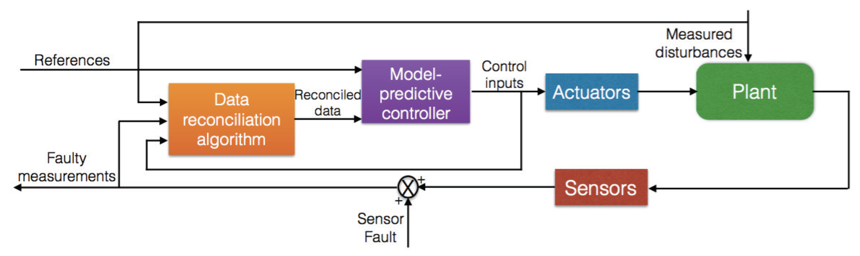
For these reasons, in this work, a fault tolerant control scheme is proposed, where a data reconciliation algorithm is included in the loop and is activated when the control system has reached the steady state. In particular, the data reconciliation unit acts in such a way that the occurred oxygen content sensor fault is made invisible to the model predictive controller, which is fed with the reconciled data. The idea of exploiting data reconciliation as a means to achieve fault tolerance in a control system is novel. Indeed, data reconciliation methods have been employed in control systems either with the goal of minimizing the noise level in process measurements or with the target of detecting faults in combination with data-based fault detection methods. In particular, in [17,18], data reconciliation was exploited to reduce the noise level in measurements and improve the performance of the control strategy for a continuous stirred tank. In [19], data reconciliation was applied with the same purpose in a distributed control system for a distillation column. Instead, in [20], data reconciliation was used in synergy with PCA for monitoring and sensor fault detection in a modelled ammonia synthesis plant. In [21], data reconciliation improved the estimation of process variables and enabled improved sensor quality control and identification of process anomalies.
As to the effectiveness of the proposed data-reconciliation based fault-tolerant control scheme, this has been shown by integrating data reconciliation with an improved version of the model predictive control (MPC) strategy earlier developed in [2] for a specific type of biomass boiler—the KPA Unicon BioGrate boiler (KPA Unicon Group Oy, Pieksämäki, Finland). Indeed, the MPC strategy presented in this work is based on a more detailed model of the BioGrate boiler, which also includes the dynamics of the oxygen content in the flue gas. The data reconciliation algorithm is based on the constrained optimization of a quadratic cost, which exploits the process static model derived from the dynamic one used for the MPC design. The performance of the overall fault tolerant control system has been evaluated by running simulations on recorded data concerning the measurement of the oxygen content in the flue gas of an actual process under faulty conditions. A schematic diagram of the integrated data reconciliation-model predictive control (DR-MPC) strategy is shown in Figure 1.
The remainder of the paper is organized as follows. Section 2 describes the process and an improved version of the MPC strategy developed in [2] for the BioGrate boiler. 
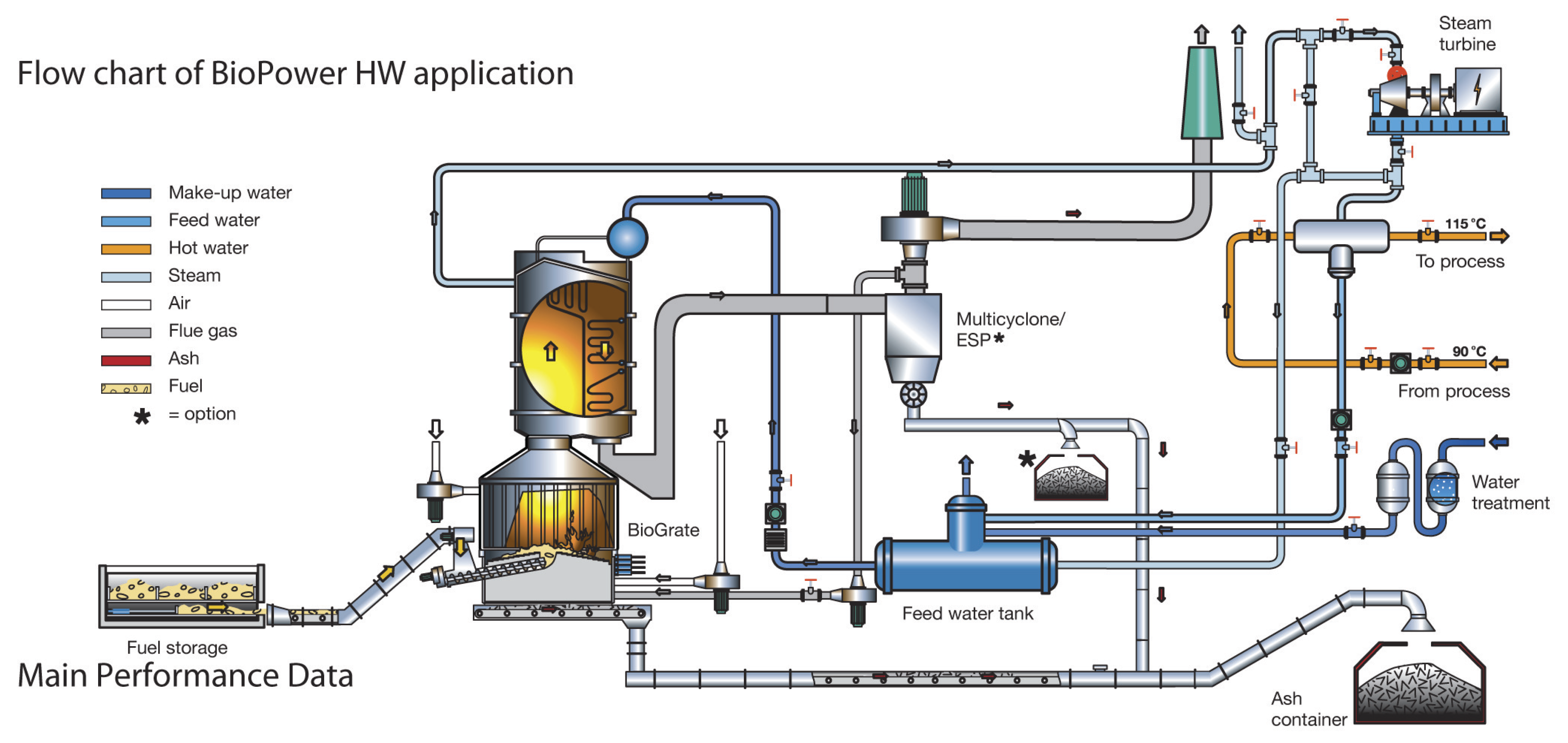
Section 2.1 provides the process description of the BioGrate boiler. Section 2.2 describes the mathematical model of the process. Section 2.3 presents the MPC strategy. Section 3 describes the data reconciliation algorithm implemented on the BioGrate boiler. Section 4 shows the effectiveness of the proposed DR-MPC strategy through the simulation results obtained by using faulty measurements recorded from the real industrial process.

2. Process and Control Description of the BioPower Combined Heat and Power Process

2.1. Process description of the BioGrate boiler

The BioGrate boiler consists of a furnace and a steam-water circulation system as illustrated in Figure 2. The furnace comprises conical-shaped grate rings that are surrounded by heat-insulating refracting brick walls. The grate consists of several rings, half of which rotate while the other half are stationary. Two consecutive rotating rings rotate in opposite directions. This setup ensures a uniform distribution of fuel throughout the grate. Fuel is fed from the bottom of the grate where it spreads towards the outer rings and undergoes combustion. The refracting brick walls radiate the heat generated during combustion back to the grate. The furnace is equipped with air register systems for combustion. Primary air flows from the bottom in a direction perpendicular to the fuel feed movement (cross-flow reactor) to ensure efficient mixing of air and fuel. The secondary air flows from the nozzles in the grate-wall to completely combust volatiles present in the over-bed region [22].
The steam-water circulation system absorbs the heat from the furnace and the flue gas to heat water-steam flowing through it. The important components of the steam-water circulation system include an economizer, a drum and evaporator system and two superheaters. The feedwater is pumped into the economizer where the water absorbs the remaining heat from the flue gas before the flue gas is released into the atmosphere. The heated water is then transferred to the drum and evaporator system. The evaporator consists of downcomers and risers that are located in the walls of the furnace. It absorbs heat from biomass combustion and produces a mixture of water and steam. The steam, separated in the drum, is then passed to the two superheaters where it is further heated with the flue gas to form superheated steam. The superheated steam is transferred to the steam turbine to generate electricity.
The main objective of the BioPower 5 CHP plant is to produce power for the generator and for the hot water network. The split ratio of 2.9 MW electricity and 13.5 MW of heat is defined by the drum pressure and turbine back-pressure. The difference between the consumed and produced power disturbs the pressure in the drum, and the control strategy equalizes the steam production and consumption by controlling the drum pressure, which is achieved by manipulating the fuel and air supply to the furnace.

2.2. Model Description of the BioGrate Boiler

The set of mathematical equations describing the process is given as ([2]):
( 1 ) x ˙ 1 ( t ) = c d s x 1 ( t ) c t h d β t h d u 2 ( t ) + c d s , i n u 1 ( t ) , ( 2 ) x ˙ 2 ( t ) = c w e v β w e v x 2 ( t ) + c w , i n d 1 ( t ) , ( 3 ) x ˙ 3 ( t ) = x 3 ( t ) + q w f ( c t h d β t h d u 2 ( t ) c d s x 1 ( t ) ) 0.0244 c w e v β w e v x 2 ( t ) , ( 4 ) x ˙ 4 ( t ) = x 4 ( t ) + d 2 ( t ) , ( 5 ) x ˙ 5 ( t ) = 1 α m e t a l ( x 3 ( t ) x 4 ( t ) ) , ( 6 ) x ˙ 6 ( t ) = x 6 ( t ) + c d s , O 2 x 1 ( t ) + c w e v , O 2 x 2 ( t ) + c t h d , O 2 u 2 ( t ) + c s a , O 2 u 3 ( t ) + c d s , i n , O 2 u 1 ( t ) ,
where x 1 ( t ) , x 2 ( t ) , x 3 ( t ) , x 4 ( t ) , x 5 ( t ) and x 6 ( t ) are the fuel bed height, the moisture content in the furnace, the power generated from the biomass combustion, the filtered steam demand, the drum pressure and the oxygen content in flue gas, respectively; u 1 ( t ) , u 2 ( t ) and u 3 ( t ) are the fuel flow rate, the primary air flow rate and the secondary air flow rate, respectively; d 1 ( t ) and d 2 ( t ) are measured disturbances and consist of the moisture content in the fuel and the steam demand, respectively; c d s , c t h d , c d s , i n , c w e v and c w , i n are model coefficients identified from process data; β t h d describes the dependence on the position of the moving grate; β w e v is the coefficient for a dependence on the position from the centre to the periphery of the moving grate; α m e t a l is a coefficient that depends on the material type of the metal tubes of the evaporator system; and c d s , O 2 , c w e v , O 2 , c t h d , O 2 , c s a , O 2 and c d s , i n , O 2 are the parameters for the linearized model of the oxygen content.
Equation (1) describes the dynamics of the amount of dry fuel in the furnace. The first two terms on the right side represent the thermal decomposition rate, whereas the last term describes the fuel feed to the furnace. Equation (2) represents the dynamics of water evaporation. The energy for the water evaporation is mainly provided by the combustion of biomass near the surface of the grate. The temperature near the bottom of the biomass layer is almost independent of the primary air flow; thus, the water evaporation rate is assumed to be independent of the primary air flow as well. Equation (3) is the equation representing the power generated from the biomass combustion. The power is a filtered difference of the power released by the fuel thermal decomposition and the power consumed by water evaporation. The second term on the right-hand side represents the power of the fuel thermal decomposition and the last term describes the power needed for water evaporation. Equation (4) represents the filtered steam demand. Equation (5) represents the dynamics of the drum pressure. The drum level is kept constant by its controller, and, therefore, the variations in the steam volume are neglected. Equation (6) describes the dynamics of the residual oxygen in the flue gas after the complete combustion.
The process models have been identified in [24], and the continuous-time state-space model of the process is:
x ˙ ( t ) = A c x ( t ) + B c u ( t ) + E c d ( t ) , y ( t ) = C c x ( t ) ,
where:
A c = c d s 0 0 0 0 0 0 c w e v β w e v 0 0 0 0 q w f c d s 0.0244 c w e v β w e v 1 0 0 0 0 0 0 1 0 0 0 0 1 α m e t a l 1 α m e t a l 0 0 c d s , O 2 c w e v , O 2 0 0 0 1 ,
B c = c d s , i n c t h d β t h d 0 0 0 0 0 q w f c t h d β t h d 0 0 0 0 0 0 0 c d s , i n , O 2 c t h d , O 2 c s a , O 2 ,
E c = 0 0 c w , i n 0 0 0 0 1 0 0 0 0 ,
C c = 1 0 0 0 0 0 0 0 1 0 0 0 0 0 0 0 1 0 0 0 0 0 0 1 .

2.3. Model Predictive Control for the BioGrate Boiler

The prime objective of the MPC strategy for the BioGrate boiler is to produce the desired amount of power for the electricity generator and for the hot water network, while maintaining the drum pressure, the fuel bed height and the oxygen content in flue gas at constant values. These variables are affected by exogenous factors such as variation in the moisture content of the fuel and the steam demand. The objective of the control strategy is achieved by utilizing the process model defined by (1)–(6) and by manipulating the air flow rates and the fuel flow rates. In order to design the MPC, a sample data model of the process has been obtained by zero-order hold discretization with sampling time T s = 1 s. Hence, from now on, we will refer to the following discrete-time system:
x ( k + 1 ) = A x ( k ) + B u ( k ) + E d ( k ) , y ( k ) = C x ( k ) .
According to (7), the k-step ahead prediction is formulated as:
y ( k ) = C A k x ( 0 ) + j = 0 k 1 H ( k j ) u ( j ) ,
where H ( k j ) contains the impulse response coefficients. Therefore, using (8), the MPC optimization problem consists in minimizing:
ϕ = 1 2 k = 1 N p y ( k ) r ( k ) Q z 2 + 1 2 Δ u ( k ) Q u 2
under the constraints:
x ( k + 1 ) = A x ( k ) + B u ( k ) + E d ( k ) , k = 0 , 1 , , N p 1 , y ( k ) = C x ( k ) , k = 0 , 1 , , N p , u min u ( k ) u max , k = 0 , 1 , , N p 1 , Δ u min Δ u ( k ) Δ u max , k = 0 , 1 , , N p 1 , y min y ( k ) y max , k = 1 , 2 , , N p ,
where r ( k ) is the target value and Δ u ( k ) = u ( k ) u ( k 1 ) . The predictions by (8) are formulated as presented in [11] and the MPC regulator problem of (9) is then solved by convex quadric programming algorithms.
The original system (7) is augmented with disturbance dynamics to achieve the offset-free tracking in the presence of model-plant mismatch or unmeasured disturbances [25]. Hence, the extended system is the following:
( 10 ) x ( k + 1 ) η ( k + 1 ) = A B d 0 A d x ( k ) η ( k ) + B 0 u ( k ) + E 0 d ( k ) + w ( k ) ξ ( k ) , ( 11 ) y ( k ) = C C η x ( k ) η ( k ) + v ( k ) ,
where w ( k ) and v ( k ) are white noise disturbances with zero mean. Thus, the disturbances and the states of the system are estimated as follows:
x ^ ( k | k ) η ^ ( k | k ) = x ^ ( k | k 1 ) η ^ ( k | k 1 ) + L x L η ( y ( k ) C x ^ ( k | k 1 ) C η η ^ ( k | k 1 ) ) ,
and the state predictions of the augmented system (10) are obtained by:
x ^ ( k + 1 | k ) η ^ ( k + 1 | k ) = A B d 0 A d x ^ ( k | k ) η ^ ( k | k ) + B 0 u ( k ) + E 0 d ( k ) .
Since η ( k ) are observable, their estimates are used to remove their influence from the controlled variables. The disturbance model is defined by choosing the matrices B d and C η . Since the additional disturbance modes introduced by disturbance are unstable, it is necessary to check the detectability of the augmented system. The augmented system (10) is detectable if and only if the nonaugmented system (7) is detectable, and the following condition holds:
rank I A B d C C η = n + n η ,
where n is the dimension of A and n η is the dimension of A d . In addition, if the system is augmented with a number of integrating disturbances n η equal to the number of the measurements p ( n η = p ) and, if the closed-loop system is stable and constraints are not active at a steady state, there is zero offset in controlled variables.

3. The Data Reconciliation Algorithm for the BioGrate Boiler

The aim of this section is to describe the data reconciliation algorithm and how it works as a fault tolerant component in the steady-state closed-loop system.
By processing the control inputs, the measured disturbances, and the measured outputs of the process—including the faulty one—the data reconciliation algorithm provides the reconciled measurements as the solution of a problem consisting in the minimization of a quadratic cost under a linear equality constraint. In addition to the measurement of the flue gas oxygen content, the other measurements benefit from corrected values. The quadratic cost is a function of the difference between the faulty measurement and the actual measurement (i.e., the fault-free value of the measurement). The linear constraint is the steady-state equation of the regulated plant, where the states which are not directly measurable are replaced by the respective soft-sensors.
In order to formally state the constrained optimization problem, the vector h ( k ) is defined as:
h ( k ) = y ( k ) x ^ 2 ( k ) x ^ 4 ( k ) u ( k ) d ( k ) ,
where y ( k ) , x ^ 2 ( k ) , x ^ 4 ( k ) , u ( k ) , and d ( k ) , respectively, are the measured outputs, the estimates of x 2 ( k ) and x 4 ( k ) , the control inputs, and the measurable disturbances. Likewise, the vector h f ( k ) is defined as:
h f ( k ) = y f ( k ) x ^ 2 ( k ) x ^ 4 ( k ) u ( k ) d ( k ) ,
where y f ( k ) denotes the faulty measured output or, more precisely, the measured output, where, in particular, the measurement of the oxygen content is affected by the fault occurred in the related sensor: i.e.,
y f ( k ) = y 1 ( k ) y 2 ( k ) y 3 ( k ) y 4 f ( k ) .
With the notation introduced in (15)–(17), the cost functional is defined as follows:
J = ( h ( k ) h f ( k ) ) W ( h ( k ) h f ( k ) ) ,
where W denotes a positive definite diagonal matrix, whose entries are identified from the indstrial data from a BioPower CHP power plant.
The linear constraint is derived from the process steady-state equations:
( A I ) x ( k ) + B u ( k ) + E d ( k ) = 0 ,
where I denotes the identity matrix, through the following reasoning. While the control input u ( k ) and the disturbance d ( k ) are directly available, the states must be replaced by their measurement—fault-free or actual ones, respectively—or by their estimates. In particular, the states x 1 ( k ) , x 3 ( k ) , and x 5 ( k ) are replaced by the fault-free measurements y 1 ( k ) , y 2 ( k ) , and y 3 ( k ) . The state x 6 ( k ) is replaced by the actual measurement y 4 ( k ) . Moreover, the states x 2 ( k ) and x 4 ( k ) are replaced by their estimates x ^ 2 ( k ) and x ^ 4 ( k ) . Hence, the linear constraint (19) can be restated in compact form as a function of h ( k ) , provided that a state-space basis transformation T is applied with the aim of re-ordering the state variables consistently with the definition of h ( k ) and the replacements described above. Namely, with T such that:
x ( k ) = T 1 x ( k ) = x 1 ( k ) x 3 ( k ) x 5 ( k ) x 6 ( k ) x 2 ( k ) x 4 ( k ) ,
and M is defined by:
M = ( A I ) B E ,
where A = T 1 A T , B = T 1 B , and E = T 1 E , (19) can be rewritten as:
M h ( k ) = 0 .
In order to minimize the quadratic cost (18) with respect to the difference h ( k ) h f ( k ) , under the linear equality constraint (20), one can straightforwardly apply the Lagrange multiplier method. Then, the Lagrangian function is:
L ( ( h ( k ) h f ( k ) ) , λ ) = ( h ( k ) h f ( k ) ) W ( h ( k ) h f ( k ) ) + λ M h ( k ) ,
where λ denotes the vector of the Lagrangian multipliers. Therefore, solving the constrained optimization problem reduces to solving the system of equations:
2 h ( k ) h f ( k ) W + λ M = 0 , M h ( k ) h f ( k ) + M h f ( k ) = 0 ,
which provides, for the reconciled variable:
h r e c ( k ) = h f ( k ) W 1 M ( M W 1 M ) M h f ( k ) .

4. Results

Two case studies are presented to demonstrate the effectiveness of the integrated DR-MPC based strategy. Simulation studies utilise industrial data from a BioPower 5 CHP power plant and the system is identified and implemented in the MATLAB (R2016b, MathWorks Inc., Natick, MA, USA) environment, as described in Section 2.2. The first case study discusses the performance of the DR-MPC during an intermittent oxygen content sensor fault. The second case study analyses the performance of the system during complete failure of the sensor.

4.1. Case Study I

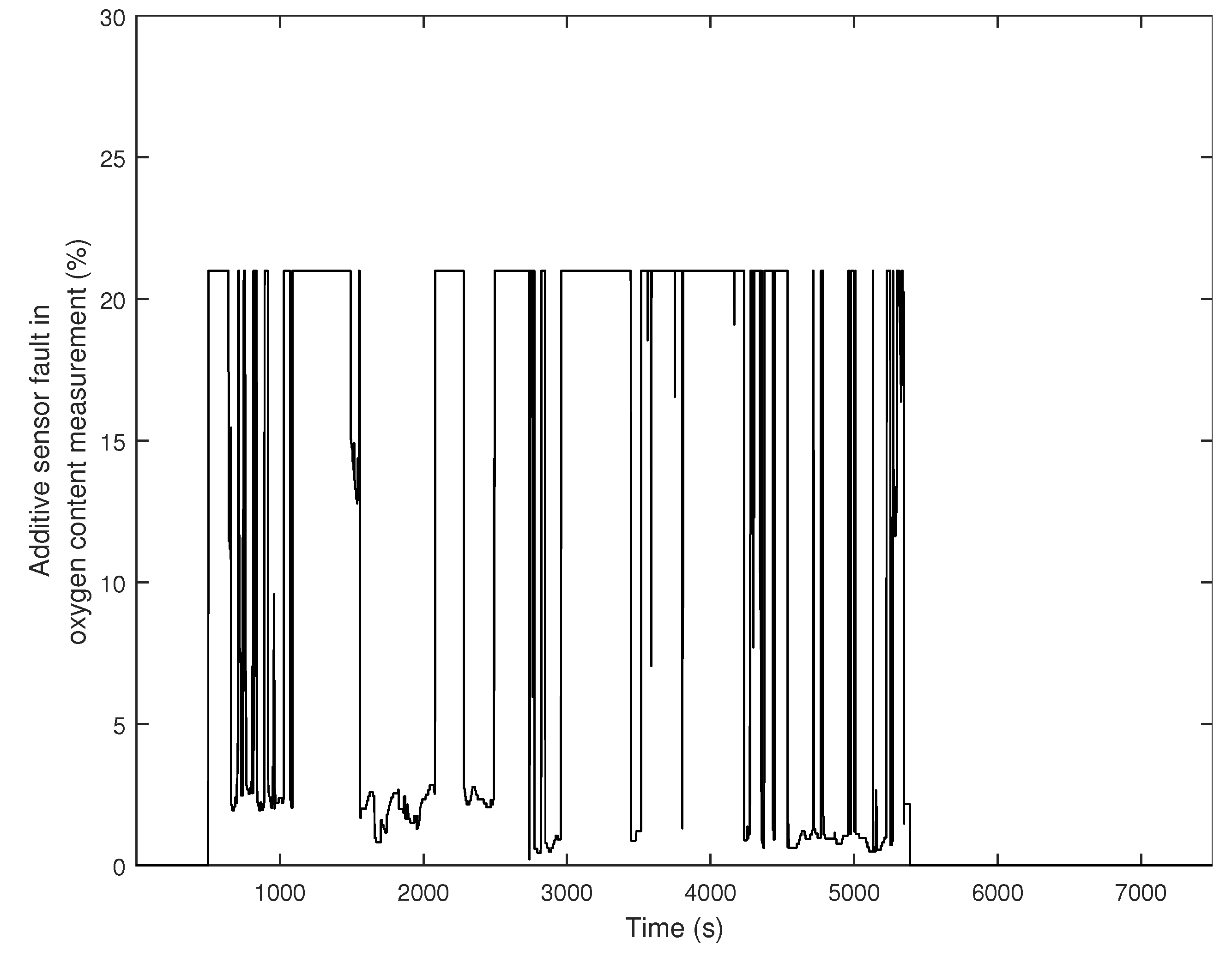
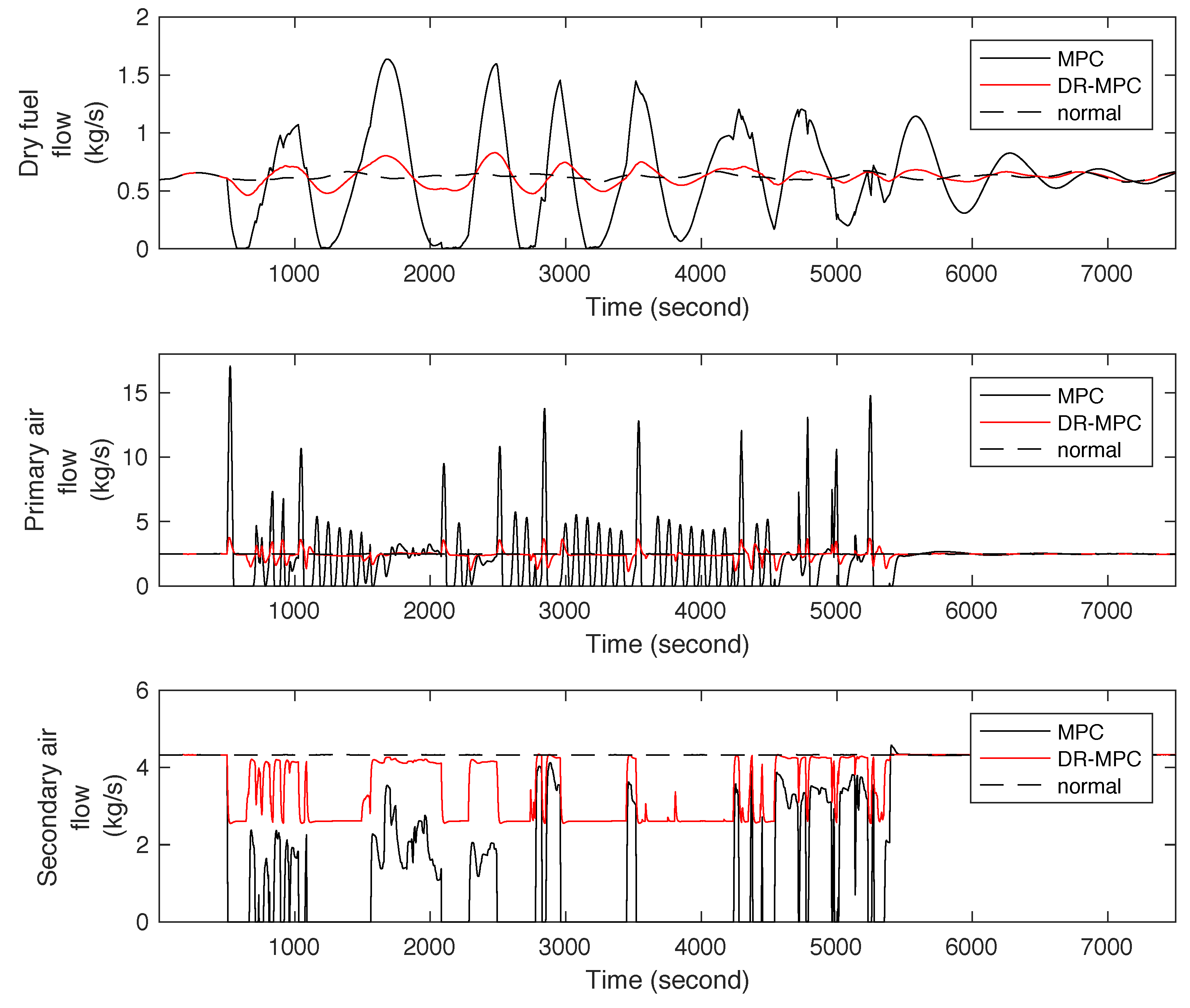
This case study describes the effectiveness of the integrated DR-MPC system during an additive intermittent fault that occurs in the flue gas oxygen content sensor from 501 s to 5400 s. The occurrence of this fault is presented in Figure 3. The effectiveness of the system is demonstrated by comparing the performances of the DR-MPC and an MPC strategy. The faultless “normal” operation of the flue gas oxygen content sensor is also demonstrated with the MPC strategy for both case studies.
In both simulation setups, the weighting matrices of the MPC controller are Q z = diag { 0.001 , 0.001 , 0.1 , 0.01 } and Q u = diag { 0.1 , 0.1 , 0.1 } , while the boundary conditions are u m i n = [ 0 0 0 ] , u m a x = [ 5 20 20 ] , Δ u m i n = [ 0.8 0.8 0.8 ] , Δ u m a x = [ 0.8 0.8 0.8 ] , y m i n = [ 0 0 0 ] and y m a x = [ 1 35 55 30 ] . The setpoint values for combustion power, drum pressure, fuel bed height and oxygen content are 15 MW, 50 bar, 0.5 m and 4%, respectively. The matrix W in the data reconciliation algorithm is defined as W = diag { 2.9914 , 3.0297 , 0.0605 , 3.0216 , 2.9852 , 2.9808 , 3.0000 , 3.0000 , 3.0000 , 3.0000 , 3.0000 } × 10 6 .
The simulation is performed for a period of 7500 s.
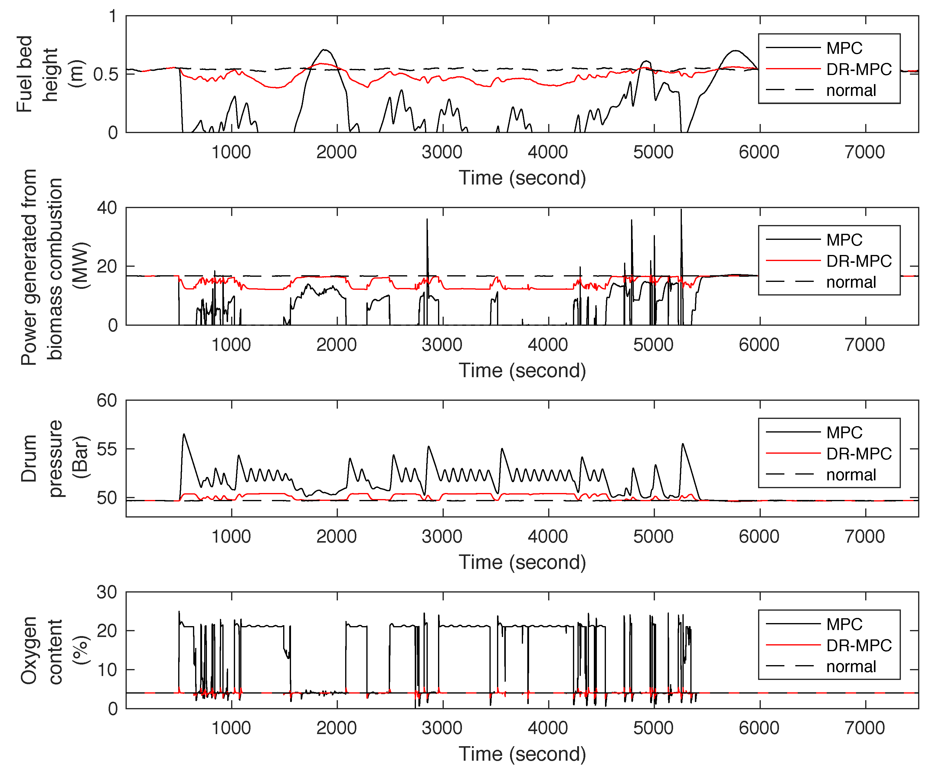
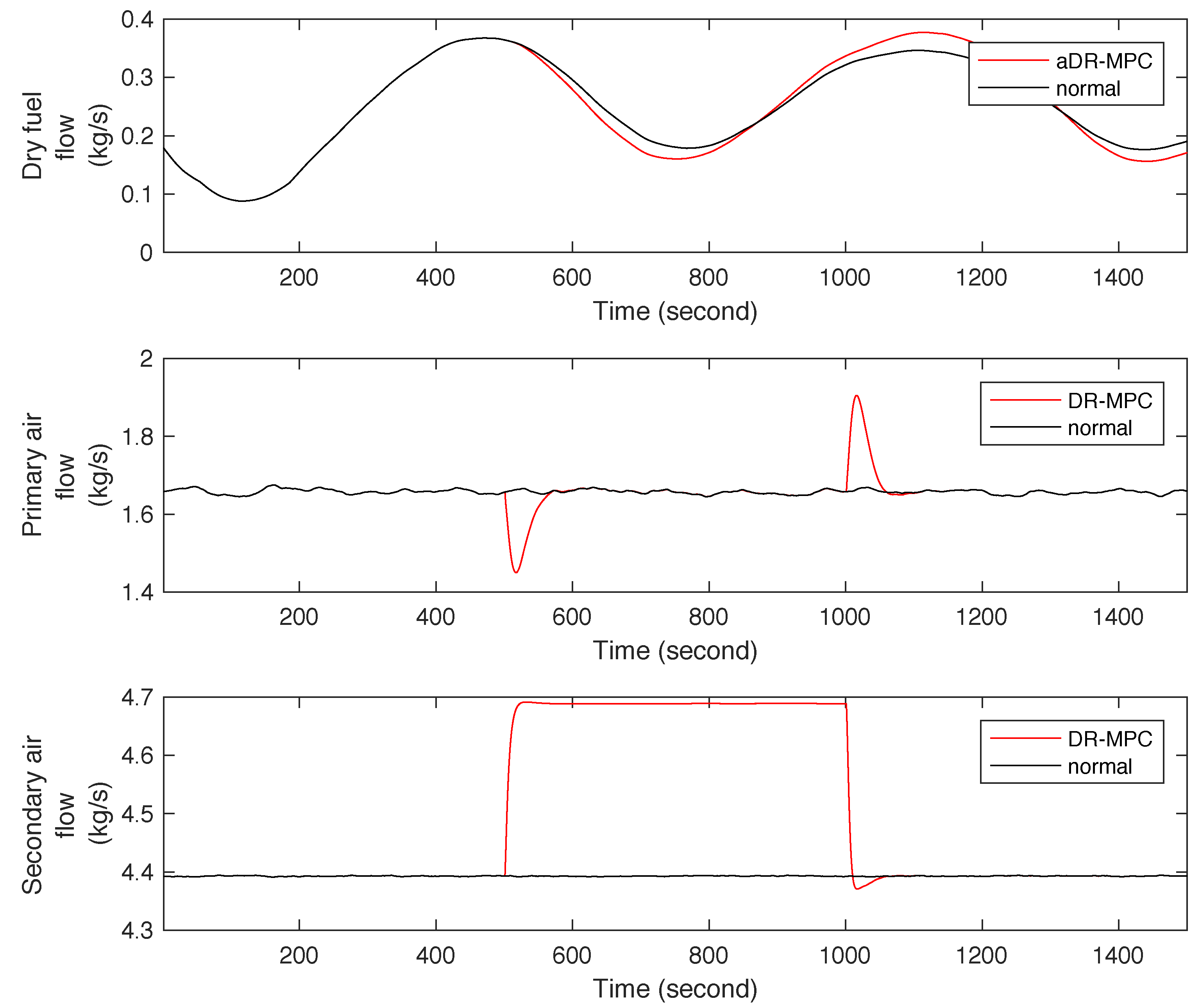
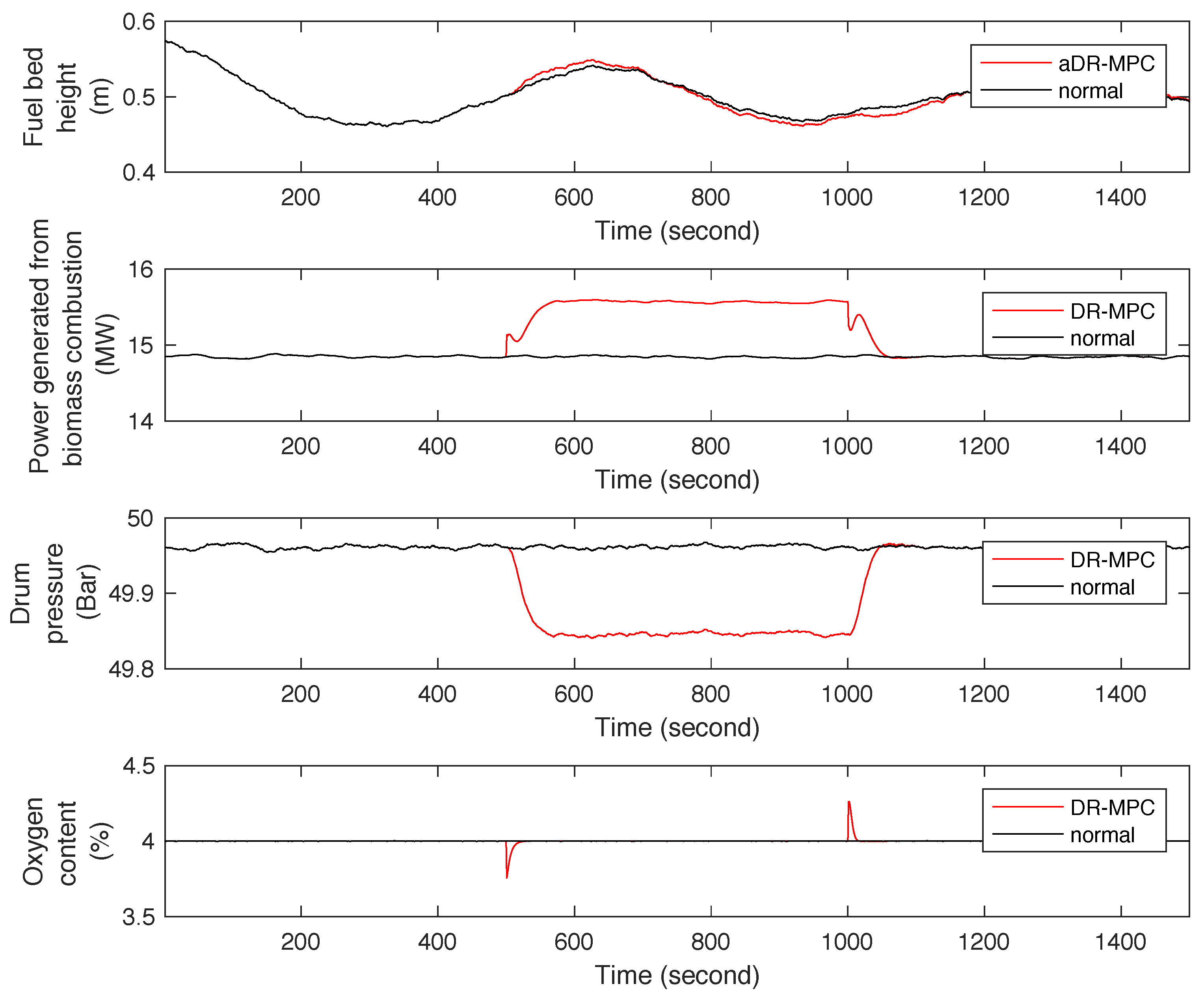
 Figure 4 and Figure 5 present the resulting behaviour of controlled outputs and control inputs, respectively. The results demonstrate that the closed-loop performance of the MPC strategy (black lines) is significantly deteriorated by the fault as it introduced undesirable oscillations to the control inputs and controlled outputs: The calculated soft-sensor value of the combustion power [24] greatly differs from its nominal value, due to the faults in the flue gas oxygen content measurement. In contrast, the integrated DR-MPC (red lines) was able to notably reduce the effects of this fault on the considered process inputs and outputs. In other words, with the data reconciliation, the fault does not affect the steady-state behavior of the system. The integrated DR-MPC works as follows: Firstly, Equation (21) is used to calculate the reconciled measurements shown in Figure 4. Secondly, Equation (12) is utilized to estimate the states and the disturbances of the system. Thirdly, the optimization problem (9) is solved, giving the new inputs as illustrated in Figure 5. Finally, new state predictions are given by Equation (13). The oscillation of the fuel bed height is caused by the smaller weight of 0.001 used by the MPC for the fuel flow and primary air flow rates in comparison to 0.1 of the drum pressure. Moreover, there is the small degradation of the measurements with the DR-MPC in comparison to the ’normal’ faultless situation.
The flue gas oxygen content measurement is still needed: in its normal operation, it measures oxygen content fast (less than second) that is needed for fast dynamics of excess air control and to prevent pollution.

4.2. Case Study II

In this case study, the performance of the integrated DR-MPC strategy is evaluated during the occurrence of an oxygen content sensor failure. The failure occurs between 500 s and 1000 s. The tuning matrices of the MPC controller, the weighting matrix of the data reconciliation algorithm, and the input and output constraints are given the same values of the previous case study. Figure 6 and Figure 7 show the performance of the integrated DR-MPC.
The MPC strategy cannot perform under the absence of measurement data from the oxygen content sensor due to the failure. Instead, when the DR-MPC strategy is active, the reconciliation algorithm provides a reconstructed signal for the oxygen content measurement. As a result, the closed-loop system is prevented from being unstable. When comparing DR-MPC with the other available methods, usually the controller reconfiguration is needed.
In summary, the case studies demonstrated that the fault effects on the BioPower process, originating from the oxygen content sensor malfunction, can be effectively minimised by integrating the data reconciliation method into the MPC strategy.

5. Conclusions

In this paper, we have introduced an integrated DR-MPC strategy to achieve a control system for the BioPower 5 CHP plant with the property of being tolerant to faults or a complete breakdown of the flue gas oxygen content sensor.
The DR-MPC strategy presented in this work was based on a more detailed model of the BioGrate boiler, which also includes the dynamics of the oxygen content in the flue gas. The data reconciliation algorithm provided the reconciled measurement as the solution of a problem consisting of the minimization of a quadratic cost under a linear equality constraint in the MPC strategy.
The effectiveness of the DR-MPC strategy has been shown by considering both an intermittent fault in the flue gas oxygen content sensor and its failure. The results showed that the closed-loop performance of the MPC strategy was significantly deteriorated by the fault as it introduced undesirable oscillations to the control inputs and controlled outputs. In contrast, the integrated DR-MPC was able to notably reduce the effects of this fault on the considered process inputs and outputs. In the case of the complete breakdown of the oxygen content sensor, the reconciliation algorithm provided a reconstructed signal for the oxygen content measurement .

Acknowledgments

This work was done as a part of the “Integrated condition-based control and maintenance” (ICBCOM) consortium project of the Finnish Funding Agency for Technology and Innovation (TEKES).

Author Contributions

Palash Sarkar conceived and designed the data reconciliation algorithm; Jukka Kortela identified the models and developed the model predictive control; All authors reviewed the work and improved the paper continuously.

Conflicts of Interest

The authors declare no conflict of interest.

Abbreviations

CHPCombined heat and power
CSFACold source flow adjustment
DR-MPCData-reconciliation model predictive control
LMPCLinear model predictive control
MPCModel predictive control
MSWMunicipal solid waste
NOxNitrogen oxides
PCAPrincipal component analysis

References

  1. Aslani, A.; Helo, P.; Naaranoja, M. Role of renewable energy policies in energy dependency in Finland: System dynamics approach. Appl. Energy 2014, 113, 758–765. [Google Scholar] [CrossRef]
  2. Kortela, J.; Jämsä-Jounela, S.L. Model predictive control utilizing fuel and moisture soft-sensors for BioPower 5 combined heat and power (CHP) plant. Appl. Energy 2014, 131, 189–200. [Google Scholar] [CrossRef]
  3. Gölles, M.; Reiter, S.; Brunner, T.; Dourdoumas, N.; Obernberger, I. Model based control of a small-scale biomass boiler. Control Eng. Pract. 2014, 22, 94–102. [Google Scholar] [CrossRef]
  4. Leskens, M.; van Kessel, L.B.M.; Bosgra, O.H. Model predictive control as a tool for improving the process operation of MSW combustion plants. Waste Manag. 2005, 25, 788–798. [Google Scholar] [CrossRef] [PubMed]
  5. United States Environmental Protection Agency. National Emission Standards for Hazardous Air Pollutants for Major Sources: Industrial, Commercial, and Institutional Boilers and Process Heaters; United States Environmental Protection Agency: Washington, DC, USA, 2015.
  6. Benyó, I. Cascade Generalized Predictive Control—Applications in Power Plant Control. Ph.D. Thesis, University of Oulu, Oulu, Finland, 2006. [Google Scholar]
  7. Klimánek, D.; Sulc, B. Evolutionary detection of sensor discredibility in control loops. In Proceedings of the 31st Annual Conference of IEEE Industrial Electronics Society (IECON 2005), Raleigh, NC, USA, 6–10 November 2005; pp. 1–6.
  8. Dunia, R.; Qin, S.J. Joint diagnosis of process and sensor faults using principal component analysis. Control Eng. Pract. 1998, 6, 457–469. [Google Scholar] [CrossRef]
  9. Qin, S.J.; Li, W. Detection, identification, and reconstruction of faulty sensors with maximized sensitivity. AIChE J. 1999, 45, 1963–1976. [Google Scholar] [CrossRef]
  10. Kadlec, P.; Gabrys, B.; Strandt, S. Data-driven soft sensors in the process industry. Comput. Chem. Eng. 2009, 33, 795–814. [Google Scholar] [CrossRef]
  11. Kortela, J.; Jämsä-Jounela, S.L. Fault-tolerant model predictive control (FTMPC) for the BioGrate boiler. In Proceedings of the 2015 IEEE 20th Conference on Emerging Technologies & Factory Automation (ETFA), Luxembourg, 8–11 September 2015.
  12. Havlena, V.; Findejs, J. Application of model predictive control to advanced combustion control. Control Eng. Pract. 2005, 13, 671–680. [Google Scholar] [CrossRef]
  13. Wang, F.; Huang, Q.; Liu, D.; Yan, J.; Cen, K. Improvement of load-following capacity based on the flame radiation intensity signal in a power plant. Energy Fuels 2008, 22, 1731–1738. [Google Scholar] [CrossRef]
  14. Wang, W.; Zeng, D.; Liu, J.; Niu, Y.; Cui, C. Feasibility analysis of changing turbine load in power plants using continuous condenser pressure adjustment. Energy 2014, 64, 533–540. [Google Scholar] [CrossRef]
  15. Wang, W.; Liu, J.; Zeng, D.; Niu, Y.; Cui, C. An improved coordinated control strategy for boiler-turbine units supplemented by cold source flow adjustment. Energy 2015, 88, 927–934. [Google Scholar] [CrossRef]
  16. Kortela, U.; Lautala, P. A new control concept for a coal power plant. Control Sci. Technol. Prog. Soc. 1982, 6, 3017–3023. [Google Scholar]
  17. Leibman, M.J.; Edgar, T.F.; Lasdon, L.S. Efficient data reconciliation and estimation for dynamic process using nonlinear programming techniques. Comput. Chem. Eng. 1992, 16, 963–986. [Google Scholar] [CrossRef]
  18. Abu-el-zeet, Z.H.; Roberts, P.D.; Becerra, V.M. Enhancing model predictive control using dynamic data reconciliation. AIChE J. 2002, 48, 324–333. [Google Scholar] [CrossRef]
  19. Schladt, M.; Hu, B. Soft sensors based on nonlinear steady-state data reconciliation in the process industry. Chem. Eng. Process. Process Intensif. 2007, 46, 1107–1115. [Google Scholar] [CrossRef]
  20. Amand, T.; Heyen, G.; Kalitventzeff, B. Plant monitoring and fault detection: Synergy between data reconciliation and principal component analysis. Comput. Chem. Eng. 2001, 25, 501–507. [Google Scholar] [CrossRef]
  21. Korpela, T.; Suominen, O.; Majanne, Y.; Laukkanen, V.; Lautala, P. Robust data reconciliation of combustion variables in multi-fuel fired industrial boilers. Control Eng. Pract. 2016, 56, 101–115. [Google Scholar] [CrossRef]
  22. Yin, C.; Rosendahl, L.A.; Kær, S.K. Grate-firing of biomass for heat and power production. Prog. Energy Combust. Sci. 2008, 34, 725–754. [Google Scholar] [CrossRef]
  23. Wärtsilä Biopower. Wärtsilä Power Plants: Bioenergy Solutions; Wärtsilä: Vaasa, Finland, 2005. [Google Scholar]
  24. Kortela, J.; Jämsä-Jounela, S.L. Modeling and model predictive control of the BioPower combined heat and power (CHP) plant. Electr. Power Energy Syst. 2015, 65, 453–462. [Google Scholar] [CrossRef]
  25. Pannocchia, G.; Rawlings, J.B. Disturbance models for offset-free model-predictive control. AIChE J. 2003, 49, 426–437. [Google Scholar] [CrossRef]
Figure 1. Integrated data reconciliation-model predictive control based fault-tolerant control (FTC) system.
Energies 10 00194 g001
Figure 2. BioPower 5 combined heat and power (CHP) process [23]: 1—primary air; 2—secondary air; 3—economizer; 4—drum; 5—superheaters; 6—evaporator.
Energies 10 00194 g002
Figure 3. Additive intermittent sensor fault in flue gas oxygen content measurement.
Energies 10 00194 g003
Figure 4. Case I—Closed-loop simulation results: Controlled outputs.
Energies 10 00194 g004
Figure 5. Case I—Closed-loop simulation results: Control inputs.
Energies 10 00194 g005
Figure 6. Case II—Closed-loop simulation results: Controlled outputs.
Energies 10 00194 g006
Figure 7. Case II—Closed-loop simulation results: Control inputs.
Energies 10 00194 g007

