1. Introduction
The installation of a battery energy storage system (BESS) in a microgrid (MG) provides a variety of MG services such as compensating for fluctuations in renewable power generation sources, voltage support, and frequency regulation [
1,
2,
3,
4,
5]. The control strategy of the BESS converter plays a major role in the performance of a BESS. Converter control strategies are classified into two types: linear controllers and nonlinear controllers. The conventional linear control strategy is the proportional-integral (PI) method, which is widely researched and applied in real systems, including BESSs [
6,
7,
8]. Although the PI method is classical and practical, there are still several problems related to the design strategy of PI parameters. Firstly, the PI method is appropriate for a single-input/single-output system, whereas a BESS is a multi-input/multi-output system. Therefore it is difficult to achieve the satisfactory performance by tuning PI parameters [
9]. If the multi-loop PI strategy is adopted in a BESS, it is rather complicated to design the controller; Secondly, a BESS is a typical nonlinear system. Since the PI method design is usually based on a local linearization model or linear controller with compensation, it can only achieve reliable performance and stability in a certain range for BESS converter control [
10]. In order to address the problems of the PI method, advanced nonlinear control methods are recommended for improving BESS converter control performance [
11].
In recent years, various nonlinear control methods have been applied to the voltage-source converter (VSC) such as hysteresis control [
12], sliding-mode control [
13], backstepping design method [
14], one-cycle control [
15], and fuzzy control [
16]. These methods can achieve stronger robustness and a larger stability range compared with PI control. However, their control performance in BESSs may still be unsatisfactory due to their respective drawbacks. For instance, the switching frequency of hysteresis control is not fixed; sliding-mode control has the tremor problem; the major disadvantage of the backstepping method is the explosion of complexity; one-cycle control has a weak ability to resist load disturbances; fuzzy control has poor static characteristics, etc.
Recently the energy-based (EB) method employing the port-controlled Hamiltonian (PCH) principle has attracted more and more attention [
17,
18,
19]. This method is a novel nonlinear robust control strategy based on passivity theory. According to this theory, the passive system, characterized by no energy production, will eventually run to the lowest energy point owing to the dissipation. If the system is expected to reach another specified balance position, an appropriate amount of external energy should be injected by the control to supplement the system energy. This process is called energy shaping. Among all the energy shaping implementation methods, interconnection and damping assignment (IDA) is the most effective strategy [
20]. Unlike other nonlinear control strategies, the EB method based on IDA strategy employs the structural properties of physical systems to obtain an easily implemented control law [
21]. Compared with the conventional PI method, the EB method has superior tracking performance and can achieve stronger stability and robustness in a large region [
22]. The complex design process is the main drawback of any EB control strategy. The designer needs some experience to design the EB control, which limits the actual applications of the EB method. However, owing to its advantages in nonlinear and multivariable systems, the EB method has been studied in the field of robot motion control where it has achieved good results. Recently, some researchers have applied the EB method in the power electronics area [
22,
23,
24,
25,
26,
27]. In [
25] the EB method was used in a pulse width modulation (PWM) rectifier. Nonetheless, no comparison between the performance of the PI and EB methods was provided. In [
26] the EB method was utilized in a grid-connected converter control application. However, the authors did not consider the influence of model mismatch, neither did they provide a comparison between the PI and EB methods. In [
27] the EB method was implemented in an active power filter control application, but robustness to parameter perturbation was not taken into account. Moreover, no design method for PI control was provided, and the performance of the PI method was poor. Up to now, there are almost no papers on the application of the EB method in BESSs. Hence the major contribution of this paper is to employ the EB strategy in a BESS for improving the control performance. Additionally, the step-by-step design strategy of the EB controller is presented, which should be helpful for further studies on EB controllers.
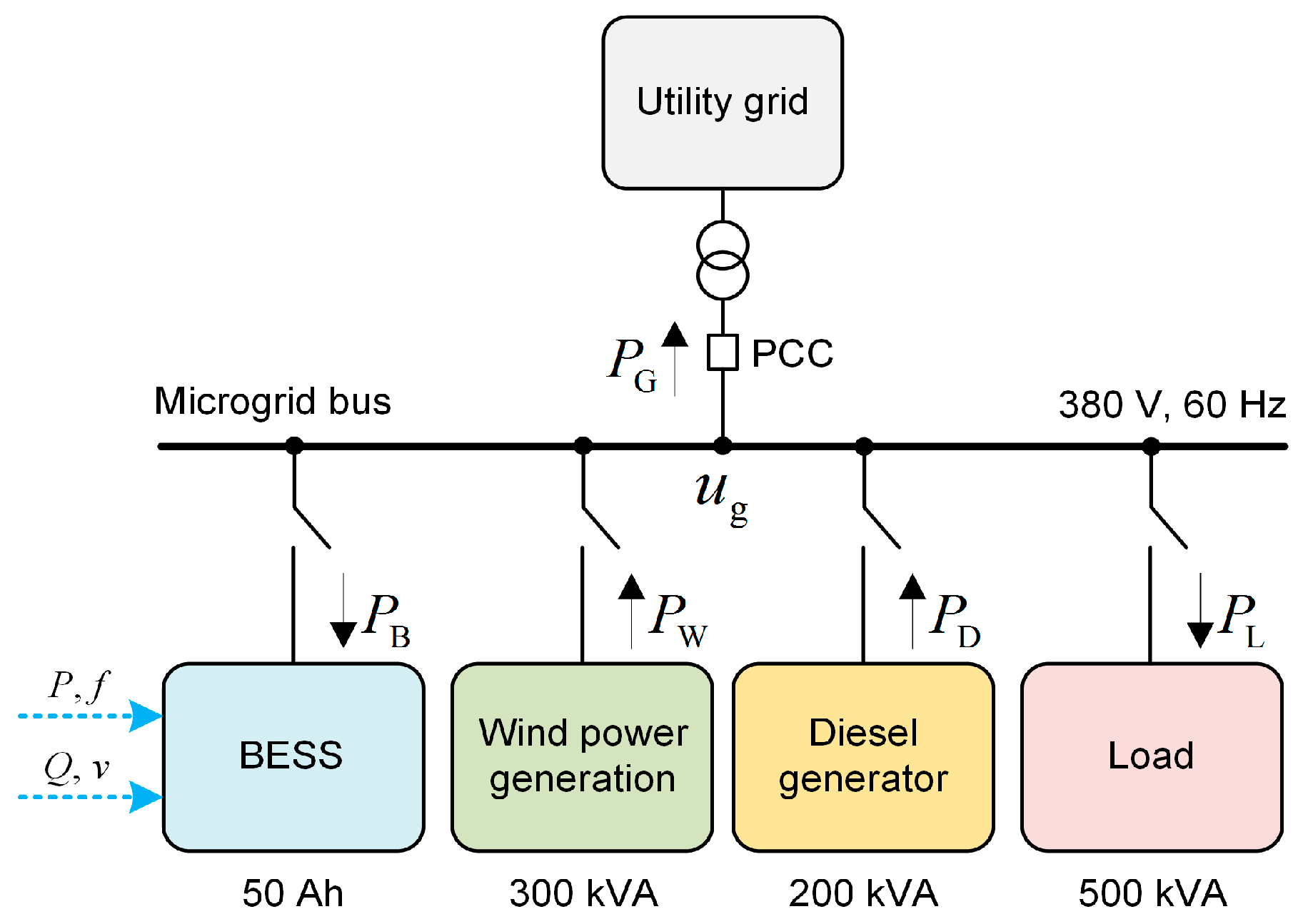
In this study, we consider a test AC MG system with a common structure including a BESS and a wind turbine generator. The BESS can be used for smoothing the wind power fluctuations in the grid-connected mode and regulating frequency in the islanded mode. The BESS consists of a converter system that is used to convert DC power to AC or DC power. Generally, the converter control system of a BESS is based on a PI regulator. In our study, the EB control strategy is used for designing the BESS controller to improve the robustness of the BESS control. The designed EB controller only depends on the converter structure of the BESS such as the DC/DC or DC/AC converters. The MG configuration has no impact on the design of the EB controller. Therefore, our proposed EB control strategy for the BESS can be applied to other MG configurations without any difficulty. In the test MG system, a common single-stage VSC structure is employed for the BESS. It should be noted that although the mathematical model of a BESS could be different due to the converter system, the design process of an EB control for other BESS structures is similar. A case study provides a detailed comparison between the performance of EB and PI control. Several cases are considered and tested by the simulation. The robustness of the EB controller against the system uncertainties is analyzed and compared with the PI control. Moreover, a sensibility analysis of the EB control method is presented to evaluate the influence of the system parameters on the control performance. The case simulation results show that stronger tracking, anti-disturbance, and robustness performance are achieved by the EB method compared to the PI method.
This paper is organized into four parts. Firstly, the structure and control scheme of the test MG system are provided in
Section 2. Secondly, the detailed step-by-step design method for the EB controller in a BESS, including the consideration of the model errors, is proposed in
Section 3. Additionally, the design method of the conventional PI controller used for comparison is briefly presented. Thirdly,
Section 4 presents the case simulation study results. By contrast with the PI control, the advantages of the proposed EB method are demonstrated. Finally, the conclusions are summarized in
Section 5.
3. Design the Current Controller of Battery Energy Storage System Using Energy-Based and Proportional-Integral Regulator
EB control is built on passivity theory. According to the definition above, the BESS is obviously a passive system, and this is because if no energy is supplemented from the power grid, the BESS will eventually run to the lowest energy point owing to the dissipation. Consequently, the EB method can be applied in BESSs naturally. In this section, the detailed step-by-step design method of EB control in a BESS is proposed. The design method of the conventional PI controller used for comparison is briefly presented too.
3.1. Design of the Energy-Based Controller Adopting the Interconnection and Damping Assignment Strategy
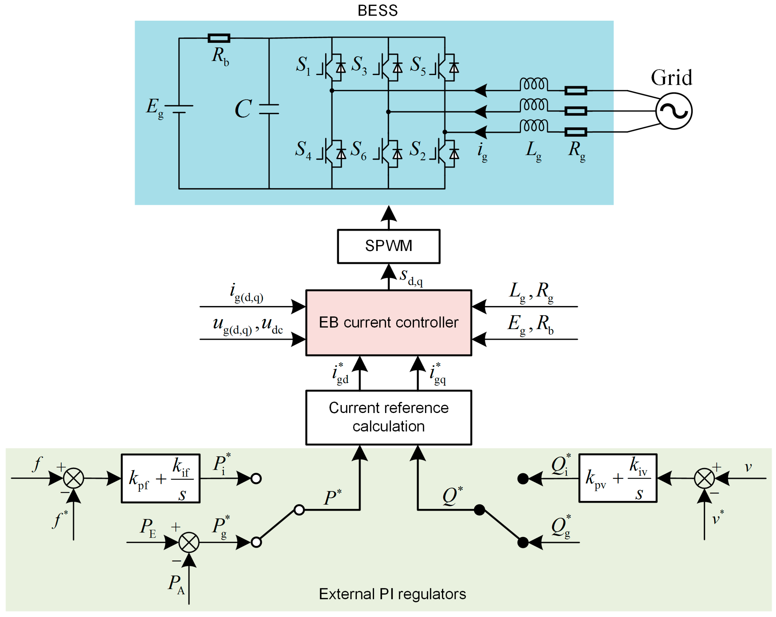
The input of the EB controller is the power reference
and
. By the current closed-loop regulation, the EB method can control the BESS power tracking with the reference power. The BESS controlled by the EB method can apply to ordinary AC MG situations. For one, BESS control is relatively independent of the power generations. Hence EB control can be implemented in different renewable production situations such as wind turbine and photovoltaic power sources. For another, BESS control is essentially a power regulation issue. In the grid-connected mode, BESS power is utilized to smooth the renewable generation output. In the islanded mode, the power references are generated by the external
f-
p and
v-
q PI controllers, which has been illustrated in
Figure 2.
The process of configuring the closed-loop system is called energy shaping in the EB control method. In this study, we adopt the IDA energy shaping strategy which is easy to implement and has respectable performance. The design of the EB controller using the IDA strategy consists of the following steps.
3.1.1. Battery Energy Storage System Modeling
The EB controller design depends on the topology of the BESS. The d-q axis mathematical model for BESS as shown in
Figure 2 is provided in Equation (2). It should be noted that the mathematical model could be different according to the converter system. Nevertheless, the design process of EB control for a BESS is similar and can be extended to the general MG configurations:
According to the IDA strategy, we need to describe a nonlinear system such as a BESS in the PCH model as:
In the PCH model, the binary product of u and y reflects the power of the system to interact with the outside. , is the internal dissipation matrix which reflects the damping characteristics of the system. J(x) and g(x) reveal the structural features of the system. H(x) describes the total stored energy in the system.
Comparing Equations (2) with (3), we can construct the PCH model for BESS as follows:
3.1.2. The Balance Point Establishment
A Hamilton function
is constructed, and it will obtain minimum at the equilibrium point
. Meanwhile, it is the desired energy function with the closed-loop feedback. In EB control, the input is
, and we should make the closed loop dissipative system as:
In Equation (7),
is a function to be determined, which is the injected energy by the control to make the system stable at the equilibrium point. To meet the above requirements, we construct the
in BESS as:
The gradient instead of the partial derivative of
x is employed in the equation. The BESS current reference in the d-q frame can be directly acquired by the power reference, which has been provided in Equation (1). The other equilibrium points of the system can be obtained by:
From Equations (1), (2) and (9) we can gain the other balance points of the system:
3.1.3. The Configuration of Undetermined Function
The suitable
and
should be identified and meet the demand of IDA strategy. Comparing the simultaneous Equations (3) and (7), and the result after simplification is:
Equation (11) is critical in the EB method design, which is used to solve the undetermined coefficients. The undetermined functions in EB controller of BESS are chosen as:
Taking the above equations into Equation (11), and after arranging we can get:
The selection of undetermined coefficients should simplify the formula and meet the Equation (14). Finally, through observation, we choose:
3.1.4. Stability Analysis
Stability issues should be considered for a controller. In order to examine the stability of the EB method, the Lyapunov second method is employed in this study. Considering that
is a positive definite energy function which is only equal to zero at the equilibrium point, it can be chosen as Lyapunov function directly, and this will simplify the stability analysis significantly. The stability of the system is dependent on the first order derivative of
:
Because
is a skew symmetric matrix, then
. Considering that
is positive symmetric matrix, it can be readily obtained:
The derivative of is negative and only equal to zero at the equilibrium point. Judging by Lyapunov second method, the balance point is asymptotically stable. Furthermore, it is evident that when . Hence a large range of asymptotic stability is achieved at the equilibrium point. It is remarkable that exceptional stability is a significant advantage for the EB method.
3.2. Combining Integral Operation
EB control may have static errors due to the impact of model errors and noise. Based on [
29], the integral action is combined to resolve this problem and increase the robustness of the system. Considering that the control variables are
and
, we need to change the positions of
and
from the internal structure matrix
J to control the input
u.
Define
. From Equation (8), it can be found
stands for the error. Hence we add a term as follows:
In Equation (21),
Z is the integral of error. It is evident that
. When
tends to zero, there is no steady error. Define:
Now a new extended PCH model is constructed:
Also, it can be obtained that:
According to [
29], all of the stability properties of
in the original PCH system are preserved in the new extended PCH system. For this extended PCH system:
After substitution, finally we can obtain:
It is worthwhile pointing out that the selection of only depends on the static error. On the whole, the primary disadvantage of EB strategy is that the initial design process of EB method is a little complex and requires experience. However, the implementation of EB method is very straightforward due to the small amount of calculation. Taken together, it is very suitable for multi-input/multi-output system like BESS.
3.3. Design of Proportional-Integral Controller
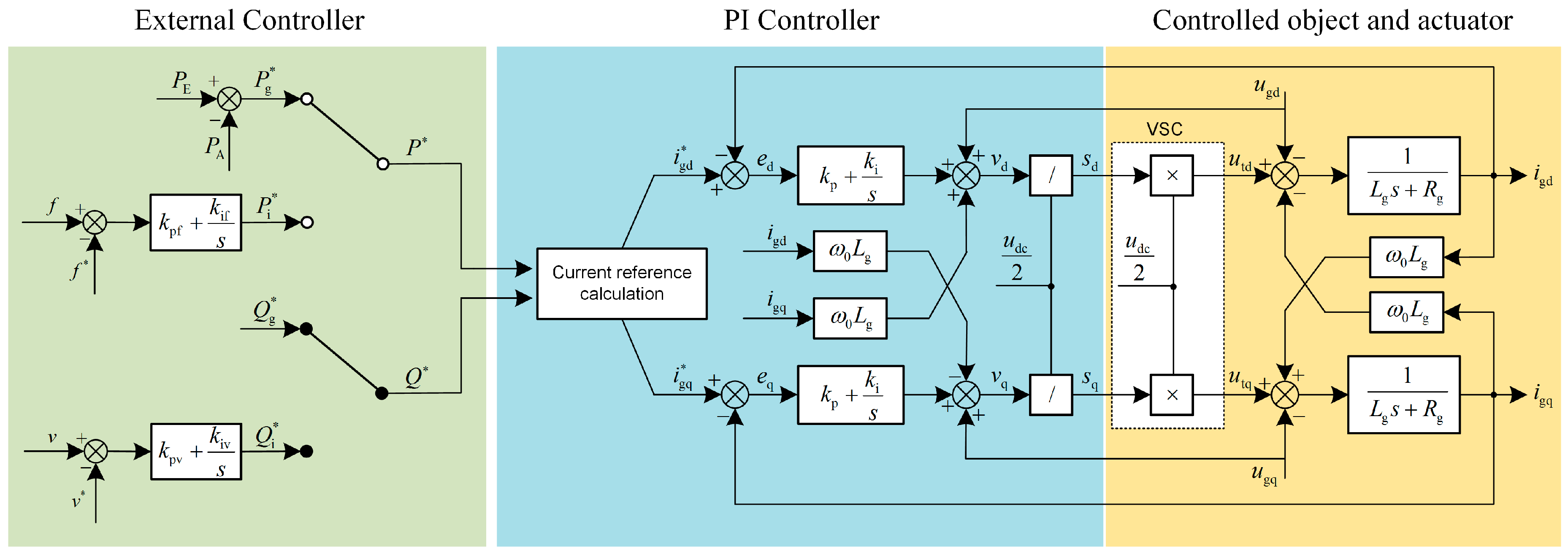
As a contrast to the EB method, the conventional PI controller should be carefully designed. The control diagram of the system in the d-q frame is illustrated in
Figure 3. In the actuator, there are two unfavorable factors for the control, which can be seen in
Figure 3. One is the coupling characteristics of the BESS current between d and q axis, and this will lead to the difficulties for the controller design. Another one is that the grid voltage is a disturbance for the BESS current control, which will deteriorate the transient performance of the system. To resolve these problems, we adopt the classic current feedforward decoupling PI control strategy [
30]. In
Figure 3,
is the current tracking error. After a PI regulator, we decouple the BESS current control in the d-q frame and feed forward the grid voltage
to restrain the disturbance.
is the sum of PI regulator output and feedforward decoupling part. Considering that VSC is equivalent to a proportional amplification, to simplify the design, we divide
by the magnification
to gain the duty ratio
, and this will make the equivalent PWM magnification
.
is the output voltage of VSC.
The classic PI parameter tuning method provided by [
30] is employed in this study. The crucial idea is that PI controller should cancel the adverse pole
. In particular, if the damping ratio
is chosen as 0.707, PI parameters can be obtained as follows:
The closed-loop transfer function is typical second order system, and the key technical indicators can be derived easily. Specifically, the overshoot is 4.3%; the phase margin is ; the rise time is , and the sheared frequency is . Overall, the system has good tracking performance and stability.
4. Case Study Results and Discussions
To verify the performance of EB control, we implemented a detailed case simulation study using the Matlab/Simulink software (MathWorks, Natick, MA. USA). In this study, conventional PI control is employed for comparison. The PI coefficients are carefully designed by the classic parameter tuning method proposed in [
30]. In the simulation, we adopt the fixed-step and ode3 algorithm. The total simulation time is 20 s. Before 1 s, the converter is not working and this period is long enough for the phase locked loop (PLL) to stabilize. At 1 s, the converter begins to work. The other related parameters in the simulation are listed in
Table 1.
Several scenarios are considered for the test MG system, including the step power tracking, ramp power tracking, grid-connected mode and islanded mode. Robustness to the parameter uncertainty must be tested due to the inevitable model mismatch. In this study, we consider two different parameter cases of
Lg and
Rg. This is mainly because it is relatively difficult to obtain accurate values for these two time-variant parameters and sometimes we even change the inductance actively to improve the performance. The result comparison of some important performance indexes in the case study is listed in
Table A1 as a supplement for the simulation figure results. After the case study, we provide a sensibility analysis to test and discuss the sensitivity of the system to the parameters.
4.1. Step Response Test
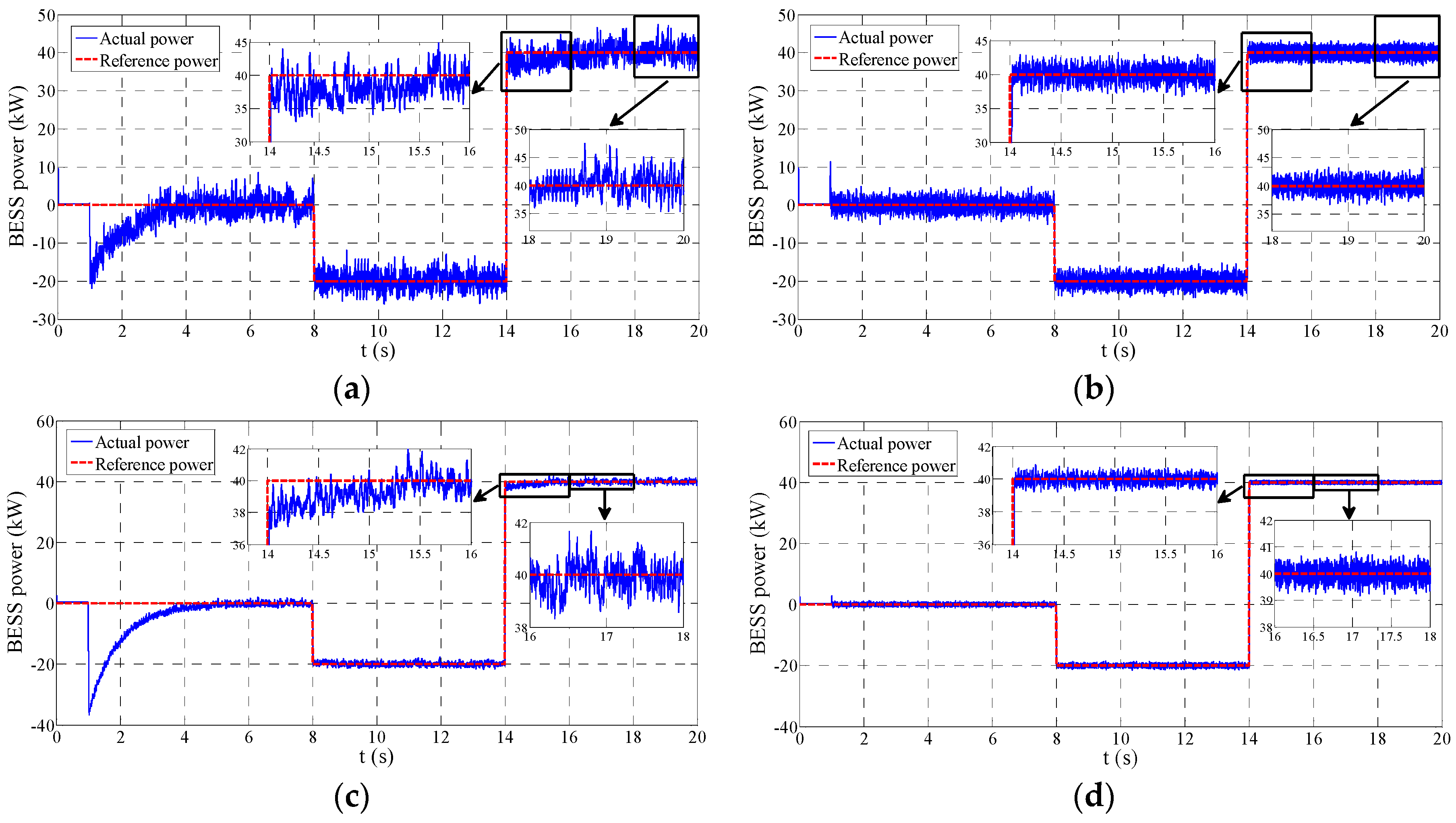
This scenario is used to test the control performance of the converter. In this scenario, the reference power is zero at first and changes to be −20, 40 kW at timepoints of 8 s and 14 s, respectively. Two different parameter cases are considered. Case A1 is the model match situation which means Lg = 1 mH and Rg = 1.1 mΩ. Case A2 is the model mismatch situation of Lg = 4 mH and Rg = 0.2 Ω.
Figure 4a,b shows the step response of the PI and EB methods in the case A1. It can be seen that both of them can track the step reference with no steady error. However, some details merit further consideration. Firstly, at 1 s, when the converter starts to work, it is equivalent to a controller disturbance. At this time, the PI method generates a larger overshoot and needs a long recovery process which lasts nearly 2.5 s. This period is defined as the adjusting time. On the contrary, the overshoot of the EB method is smaller, and the recovery process is less than 0.05 s. Therefore the EB method has a better anti-disturbance performance than the PI method. Secondly, both approaches can track the step reference with a very fast speed (less than 0.02 s) and virtually no overshoots exist. However, the PI method still needs some time to eliminate the steady error (this can be seen at 14 s), whereas the EB method avoids this process entirely. Finally, the EB method has a smoother stable performance which can be observed in the enlarged figure, and this also suggests that relatively small low-frequency harmonic and ripple peak values can be achieved by the EB method. It is worth noting that the dominant harmonic frequency of the EB method is higher than that of the PI method, whereas some additional filter device can easily absorb high-frequency ripples.
Figure 4c,d provides the step response in the case A2. It can be observed that the EB method maintains its exceptional performance both in the transient and steady state. On the contrary, the PI method has a worse recovery process compared with
Figure 4a. The overshoot increases to −36 kW and the adjusting time extends to nearly 4 s. At 14 s the PI method presents a slower tracking process.
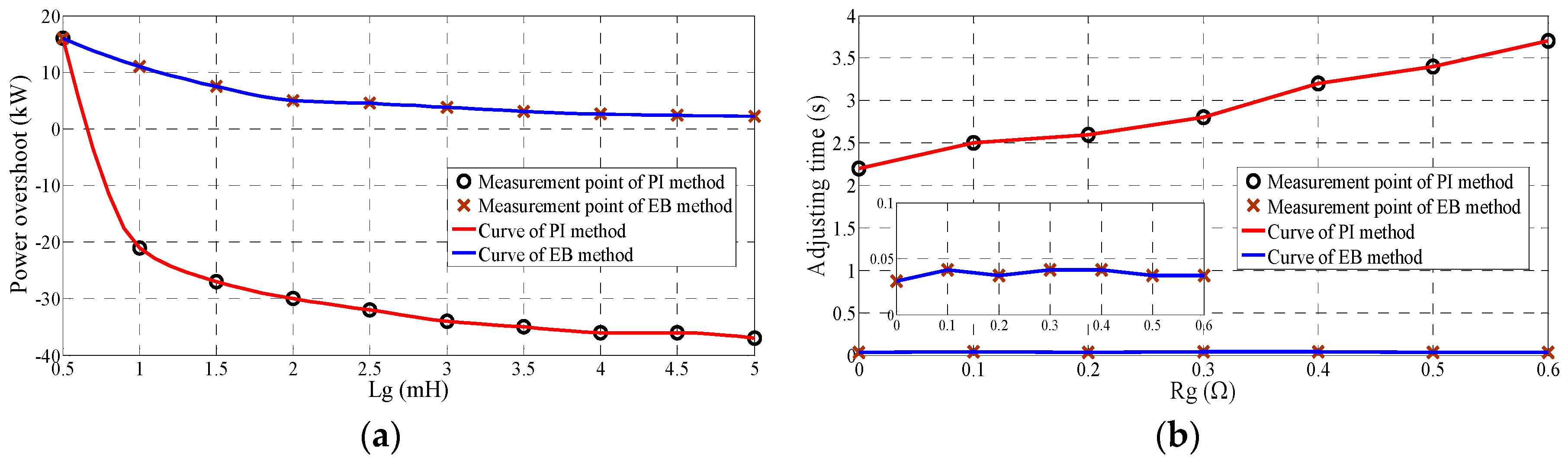
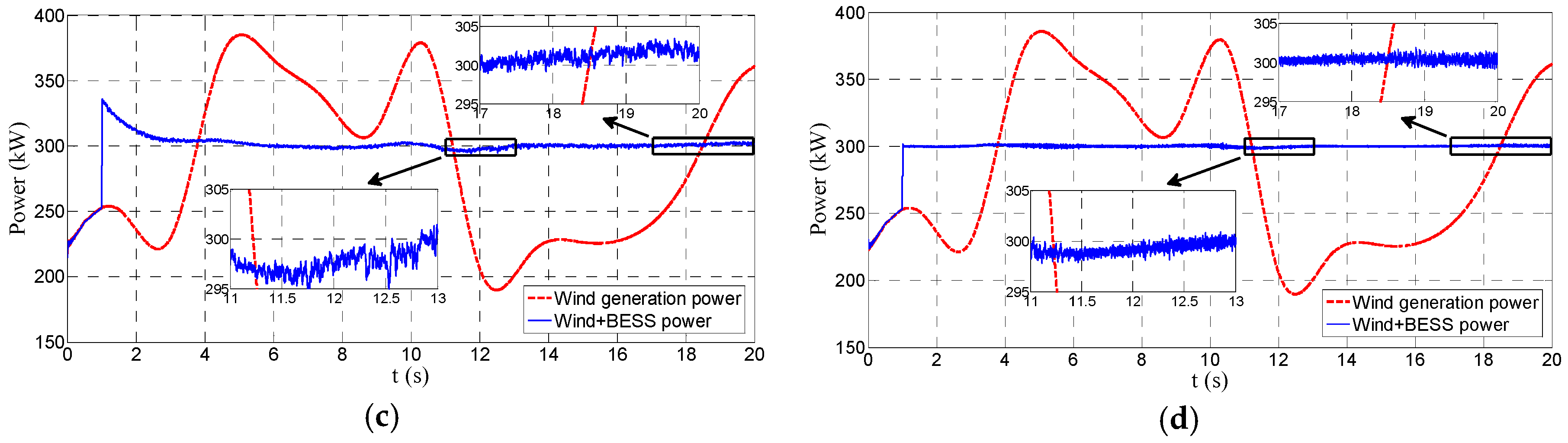
Figure 5a provides the power overshoot (at 1 s) when
Lg changes and
Rg is fixed to 1.1 mΩ.
Figure 5b shows the adjusting time when
Rg changes and
Lg is fixed to 1 mH. It can be found that the performance of the PI method is significantly affected by the parameter change whereas EB method has a superior robustness to parameter uncertainty.
4.2. Ramp Response Test
This scenario is also used to test the control performance of the converter. The converter starts at 1 s, and the reference gradually increases with the slope of 10 kW/s. Case B1 is the situation of
Lg = 1 mH and
Rg = 1.1 mΩ. Case B2 is the condition of
Lg = 4 mH and
Rg =0.2 Ω.
Figure 6 compares the slope response performance of PI and EB methods in these two cases.
It can be seen that the EB method has evidently better tracking ability compared with the PI method. Additionally, the EB method can maintain its satisfactory performance when the parameters vary. Conversely, the performance of the PI method has a significant change both in overshoot and adjusting time.
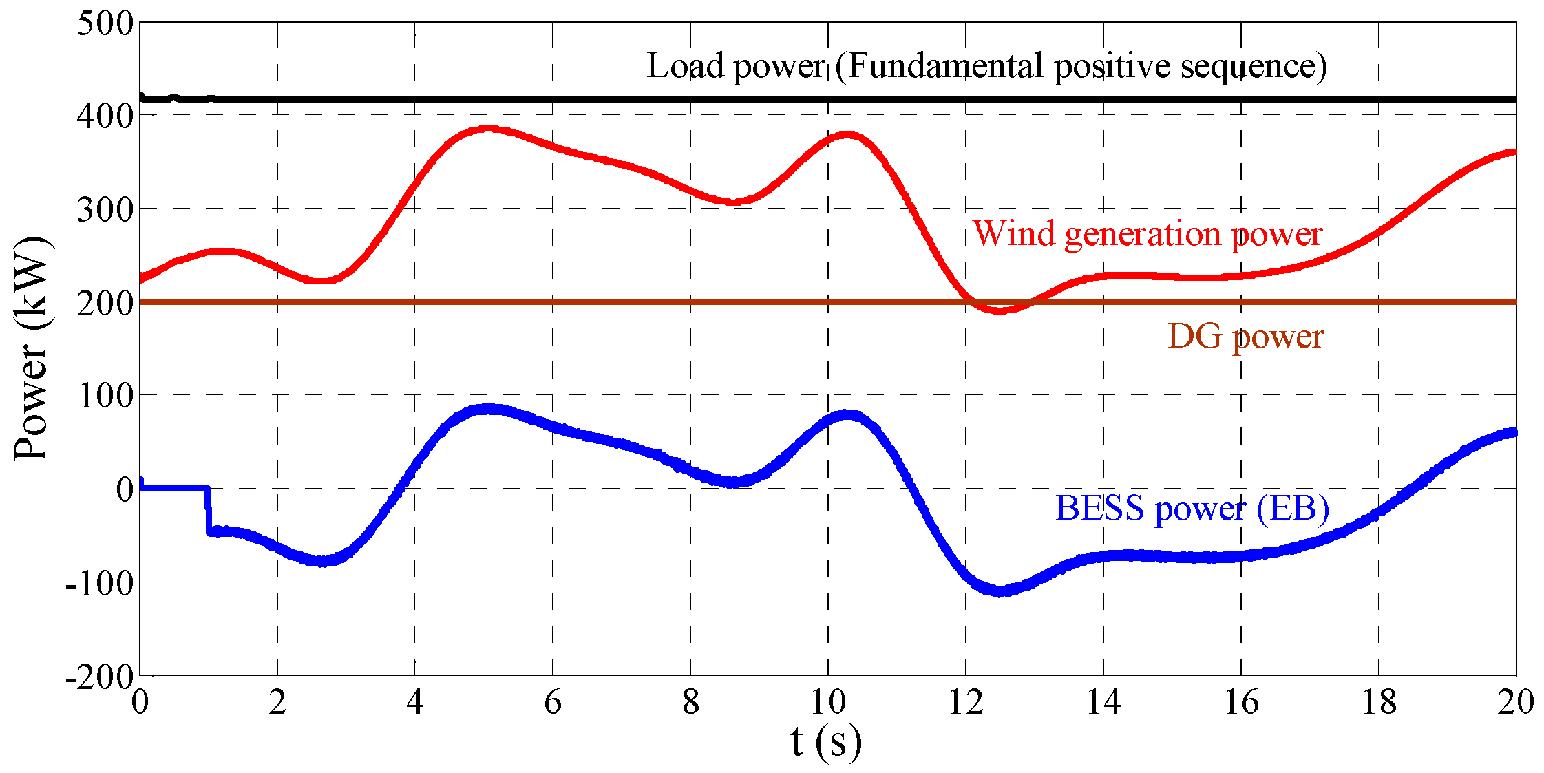
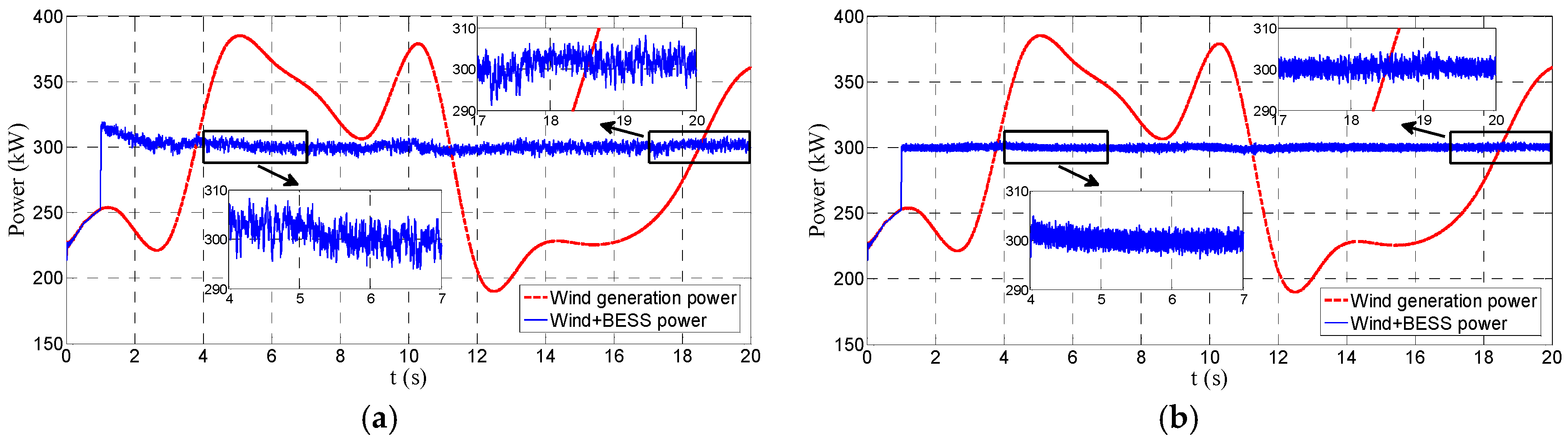
4.3. Grid-Connected Mode Test
Figure 7 shows the power of some main parts of the MG in grid-connected mode test. In this scenario, the fluctuation of the wind generation power is illustrated in
Figure 7. We have defined the charging direction of
is positive as shown in
Figure 1. Hence the fluctuation of
has the same direction with that of wind generation. The load includes linear and nonlinear parts. Linear part is the resistor of 350 kW, and the nonlinear element is a capacitor filtered diode rectifier circuit with a
resistor in DC side. Case C1 is the model match situation which means
Lg = 1 mH and
Rg =1.1 mΩ. Case C2 is the model mismatch situation of
Lg = 4 mH and
Rg = 0.2 Ω.
Figure 8a,b compares the performance of smoothing the fluctuations in wind generation between the EB and PI methods in the case C1. When the converter starts to work at 1 s, the PI method has a disturbance recovery process and the adjusting time is about 2.7 s, whereas the EB method goes into the steady state very fast and almost no overshoot exists.
Furthermore, when the PI method is in the steady state, it shows an obvious slight low-frequency fluctuation. However, the EB method provides a much smoother performance.
Figure 8c,d shows the smoothing performance in the case C2. The EB method keeps the good performance whereas the performance of the PI method is unsatisfactory. It can be noticed that smoothed power of EB method is much flatter than that of the PI method. Moreover, the overshoot of the PI method at 1 s increases to be near 36 kW and the adjusting time is over 4 s.
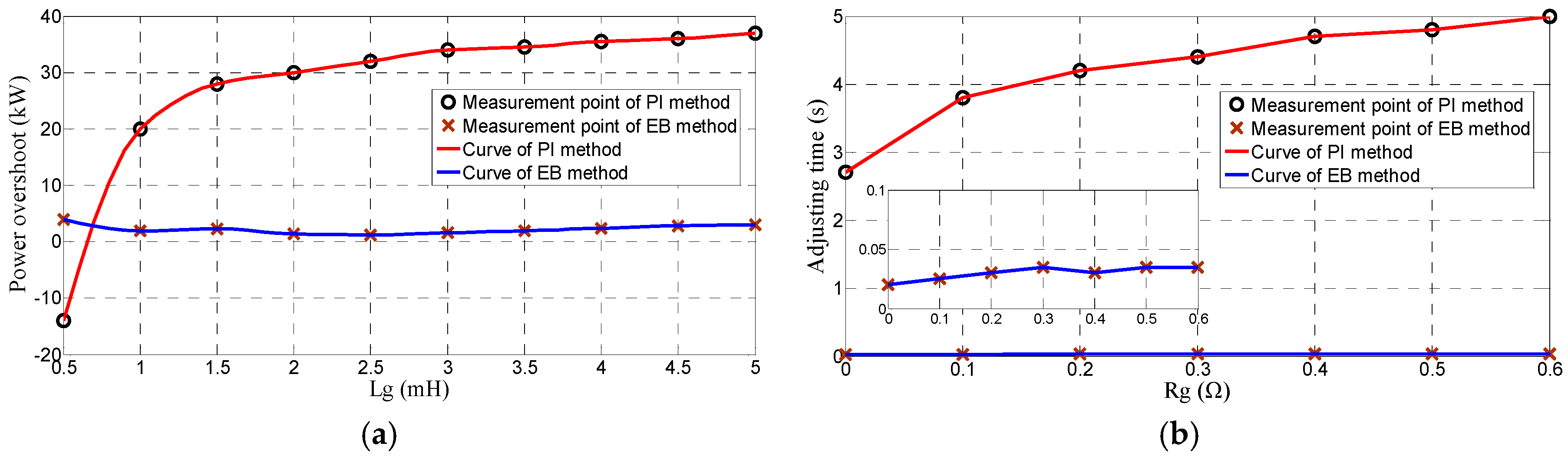
Figure 9a,b provides the overshoot and adjusting time when
Lg and
Rg vary, respectively. It can be found that the EB method has a better robustness to parameter uncertainty and the parameters greatly influence the performance of the PI method.
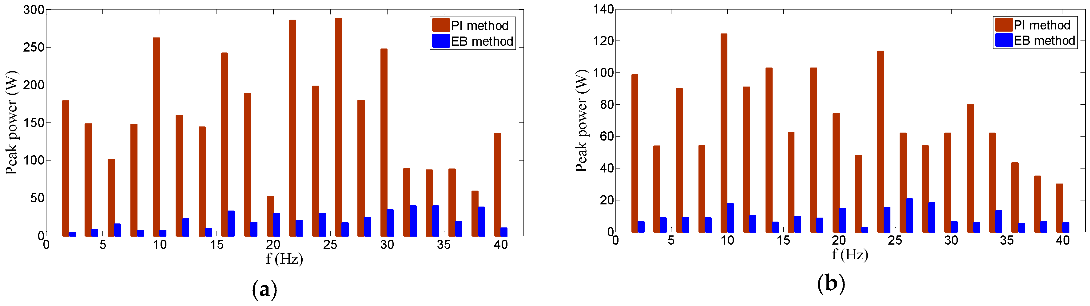
Figure 10 provides the comparison of the low-frequency ripple of the smoothed power between the PI and EB methods during 12–20 s in cases C1 and C2. It can be seen that the smoothed power of the PI method has much more low-frequency ripples than that of the EB method, and this is mainly because the tracking ability of the PI method is insufficient, especially when wind generation changes steeply. In the case C1, the total ripple root mean square (RMS) value of smoothed power by the PI method is 2.5 kW, whereas it decreases to 1.05 kW by the EB method. In the case C2, the whole ripple RMS value of smoothed power by the PI method is 1.6 kW, whereas it is only 0.6 kW for the EB method. Also, it is found that the EB method has a smaller peak ripple value compared to the PI method.
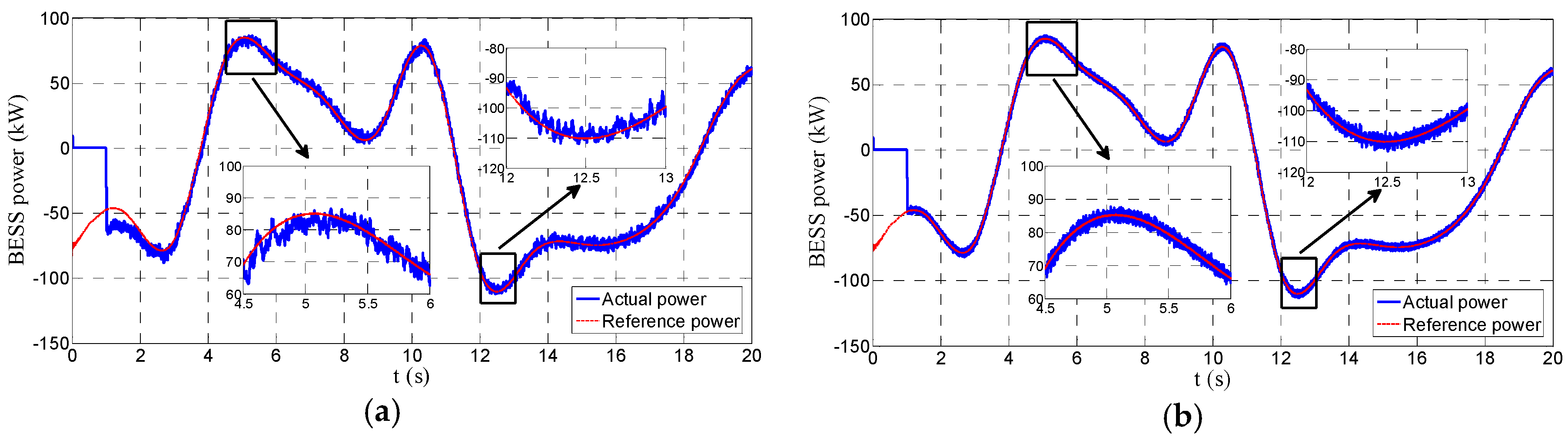
Figure 11 depicts the power tracking performance in the case C1. It can be seen that both the PI and EB methods can follow the reference well. However, the EB method has a stronger tracking capability with a smaller ripple. In particular, there is some tracking error for the PI method when the reference abruptly varies, which is shown in the detailed figure. However, the EB method avoids this problem. Besides, the PI method needs a disturbance recovery process whereas the EB method tracks very fast. Consequently, the anti-disturbance and tracking ability of the EB method are preferable to those of the PI method.
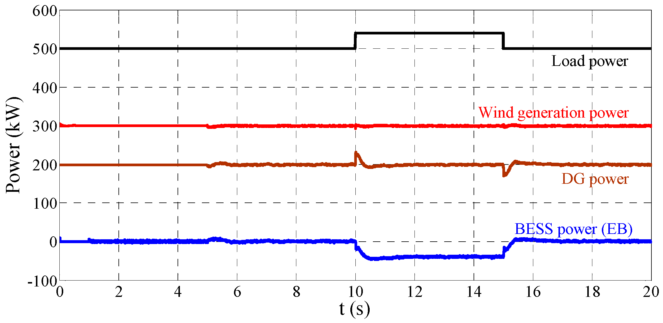
4.4. Islanded Mode Test
BESSs are utilized to regulate the frequency and voltage in the islanded mode. The real power and reactive power references of a BESS are generated by extra
f-
p and
v-
q PI controllers, respectively. In this scenario, we assume the wind generation is constant at
and the initial load is
. At 5 s the MG goes into islanded mode; at 10 s a
resistor is connected to the MG, and it is disconnected at 15 s.
Figure 12 provides the power of some principle components of the MG in the islanded mode test.
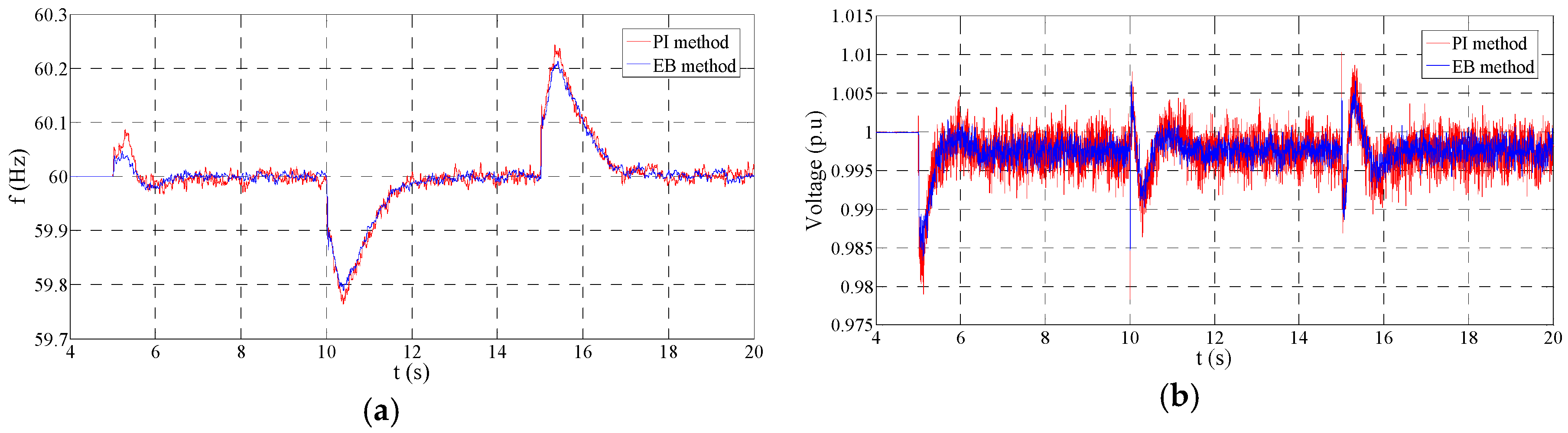
Figure 13a compares the frequency regulation performance between the PI and EB methods, and
Figure 13b demonstrates the contrast on voltage regulation. The performance of the PI and EB controllers is quite similar because the control performance mainly depends on the external
f-
p and
v-
q PI controllers and their outer PI controllers are the same. However, it can be found that the EB controller has a better transient performance and a lower ripple compared with the PI method.
4.5. Sensibility Analysis
To analyze the influence of system parameters on the control performance, we implement a sensibility test for the designed controllers. Both of the grid-connected mode and islanded mode are considered. To evaluate the sensitivity levels of the system to parameter variations, we define the sensitivity analysis factor (
SAF) [
31] as:
In Equation (28), is the variation ratio of evaluation index; represents the change rate of the uncertainties. When SAF > 0, it means that the evaluation index and uncertainty factors change in the same direction; when SAF < 0, they are indicated to vary reversely. The larger is, the evaluation index A is more sensitive to the uncertainty F. The change extent of F is not important, and we are mainly concern about the SAF to the parameter change.
In the grid-connected mode, we select the peak-ripple factor (
PRF) of the smoothed power as the evaluation index, for it can indicate not only the smoothness degree, but also the ripple level. We define the
PRF as:
In Equation (29),
is the peak-to-peak value of the smoothed power;
is the average value of the smoothed power. The lower
PRF is, the smoother power and smaller ripples are achieved. The actual conditions should determine the tolerance level of
PRF. We choose the tolerance margin of
PRF to be 8% in this study which corresponds to a maximum ripple peak-to-peak power of 24 kW. We change several critical system parameters and test the
SAF performance in EB control system. The test results are shown in
Table 2.
From
Table 2, we can find the
PRF performance is not sensitive to the variation of
,
,
,
and
. It is moderately sensitive to the battery nominal voltage
because the control performance has a relationship with the DC voltage. Nevertheless, when
increases by 10% and reaches 880 V which is a very high value for the real system, the
PRF value is still very low. The most sensitive factor is the
in the grid-connected mode.
Figure 14 compares the steady-state
PRF performance between PI and EB methods when
changes. It is worthy to note that the disturbance recovery process of PI method is excluded from the test range. To meet the demand of
PRF < 8%, we should choose
for the EB controller and
for the PI controller.
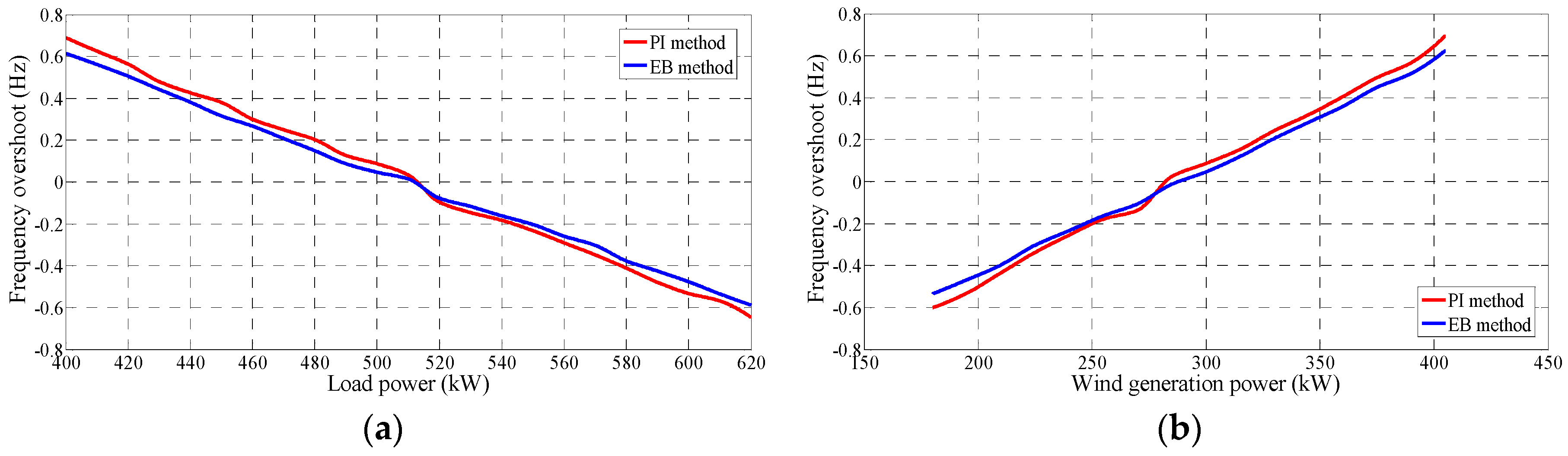
In the islanded mode, we select the frequency overshoot value
during the mode transition period (from 5 s to 6 s) as the evaluation index.
is defined as the difference between the peak frequency and the fixed frequency. The tolerance margin is determined as
in this study. The
SAF performance to the parameter variety in EB control system is provided in
Table 3. We can find the most sensitive parameters are the initial load power
and the wind generation power
.
Figure 15 demonstrates the frequency overshoot when these two parameters vary. To ensure the overshoot within the tolerance region, we can change the load power from −14.54% to 18.68% for the PI control method. Whereas in EB control system the load variation region can be from −15.82% to 20.6%. The wind generation power can change from −33.2% to 25.27% for the PI method. Whereas it can vary from −37.3% to 29% in EB control system. The permitted change area of EB method is larger than that of the PI method.
5. Conclusions
In this study, EB method is applied in BESS to overcome the inherent drawbacks of the PI method and improve the control performance. Detailed step-by-step design method based on IDA strategy has been presented. Firstly, we have constructed the PCH model of BESS. Then the equilibrium point of control variable was solved. Afterward, the undetermined matrix was calculated and acquired. Finally, integral action has been combined to enhance the robustness of the EB method.
Case simulation results have demonstrated that the EB method has better performance both in the steady and transient state than PI method. Specifically, EB method has three advantages compared with the traditional PI method. Firstly, EB method has better tracking ability than PI method. EB method has a superior steady-state performance and a smaller ripple for the smoothed power. Secondly, EB method has better anti-disturbance capability than PI method. In the simulation, the PI method has a slow disturbance recovery process with a significant overshoot. Conversely, EB method only has a slight overshoot and nearly avoids the disturbance recovery process. Finally, EB method has the superior robustness to parameter uncertainty. The performance of the PI method is affected by parameters substantially, whereas EB method maintains a satisfactory performance.
Although the performance of EB control is better than PI control, the main drawback of EB control method is the higher design complexity, which limits the application of EB control in the power converters. However, the implementation of the EB control method is straightforward. The step-by-step designing process of EB control proposed in this study would be useful for the person who wants to study the EB control. The proposed EB control for the BESS does not depend on the MG configuration. The proposed method could be easily applied to the other MG configurations.


