A Heuristic Diagnostic Method for a PV System: Triple-Layered Particle Swarm Optimization–Back-Propagation Neural Network

Abstract

This paper proposes a heuristic triple layered particle swarm optimization–back-propagation (PSO-BP) neural network method for improving the convergence and prediction accuracy of the fault diagnosis system of the photovoltaic (PV) array. The parameters, open-circuit voltage (V_oc), short-circuit current (I_sc), maximum power (P_m) and voltage at maximum power point (V_m) are extracted from the output curve of the PV array as identification parameters for the fault diagnosis system. This study compares performances of two methods, the back-propagation neural network method, which is widely used, and the heuristic method with MATLAB. In the training phase, the back-propagation method takes about 425 steps to convergence, while the heuristic method needs only 312 steps. In the fault diagnosis phase, the prediction accuracy of the heuristic method is 93.33%, while the back-propagation method scores 86.67%. It is concluded that the heuristic method can not only improve the convergence of the simulation but also significantly improve the prediction accuracy of the fault diagnosis system.

1. Introduction

The latest report from the International Energy Agency shows that, with the rapid development of photovoltaic (PV) technology, PV has become a major actor in the electricity sector in several countries; 1.3% of the world’s electricity generation is covered by PV up to January 2016 [1]. With the increase in the scale of PV power generation and the instability of the working surroundings, PV faults become more serious and are attracting wide attention. Faults affect a PV system’s performance and reliability. The causes of PV system faults are mainly temperature fault, partial shading fault, modules aging, the open-circuit or short-circuit of PV modules, and cell damage [2,3,4]. Temperature faults mainly stem from the PV modules’ high surface temperature after absorbing sunlight in contrast to PV array partial shading faults, which are either unpreventable but fluctuating, like clouds, or eliminable, such as fallen leaves and dust. Short-circuit and open-circuit faults are mainly caused by aging problems of PV modules after long-term operation. Determining the fault type in a PV system quickly and effectively is important to maintaining safe and reliable PV power generations.

Several diagnostic methods for PV system have been introduced by scholars, as follows:

Takashima et al. proposed two kinds of fault diagnosis methods for PV arrays: time domain reflectometry (TDR) and earth capacitance measurement (ECM) [5,6]. In the TDR method, with the aid of a normative pulse pump signal in the series PV array, the change in the reflected electrical property is used to judge the fault type [5]. In the ECM method, the earth capacitance of the series PV array is used to determine the module’s fault in the PV array [6].

Chao et al. developed a portable fault diagnosis meter by applying an extension neural network, chip microcontroller and a ZigBee wireless sensor network module [7]. In the method proposed by Chao et al., the fault characteristics of PV array in different fault conditions were obtained first by simulation, after which the real-time illumination and module temperatures were extracted. The data from the simulation and experiment were imported into the extension neural network as the weight matrix to identify the fault types.

Hsieh et al. proposed an intelligent fault diagnostic scheme based on the theory of chaotic signal synchronization [8]. In their diagnostic scheme, MATLAB (Manufacturer: Natick, MA, USA) was used to establish a PV system under different fault conditions. The fault characteristic parameters from the current–voltage (U-I) curve of the PV system were used and recorded, the dynamic error of the fault signals was derived by chaotic signal synchronization, and the captured output voltage signal was used as the recognition characteristic to determine the fault type.

A fault diagnostic method for a PV system based on a back-propagation (BP) artificial neural network has also been proposed [9]. An artificial neural network [10] is a machine learning mechanism for simulating how the human brain learns and identifies problems, and is applicable to fault diagnosis. The BP neural network is the common approach [9,10,11,12,13], being a multilayer fed forward network of three or more layers. The forward network is trained by an error back propagation algorithm, and the front- and back-layer neurons are connected by different weights; however, there is no connection between the neurons of the same layers. In the BP method, when the learning mode is provided to the training network of the BP, the activation value of the neuron is delivered from the input layer to the output layer via the hidden layers, and the input responses of the network are reflected in each neuron of the output layer. The connection weights are revised from the output layer to the input layer via the hidden layer, with the aim of reducing error between the expected and the actual value. With the correction of the error, the accuracy of the input responses of the BP neural network also increases. However, the disadvantage in a BP neural network is that a sample database with large volumes and long training periods is required for convergence. Additionally, improper sample selection or a longer training phase can lower prediction accuracy of a PV fault diagnosis system.

The contributions of our work are:

(1)

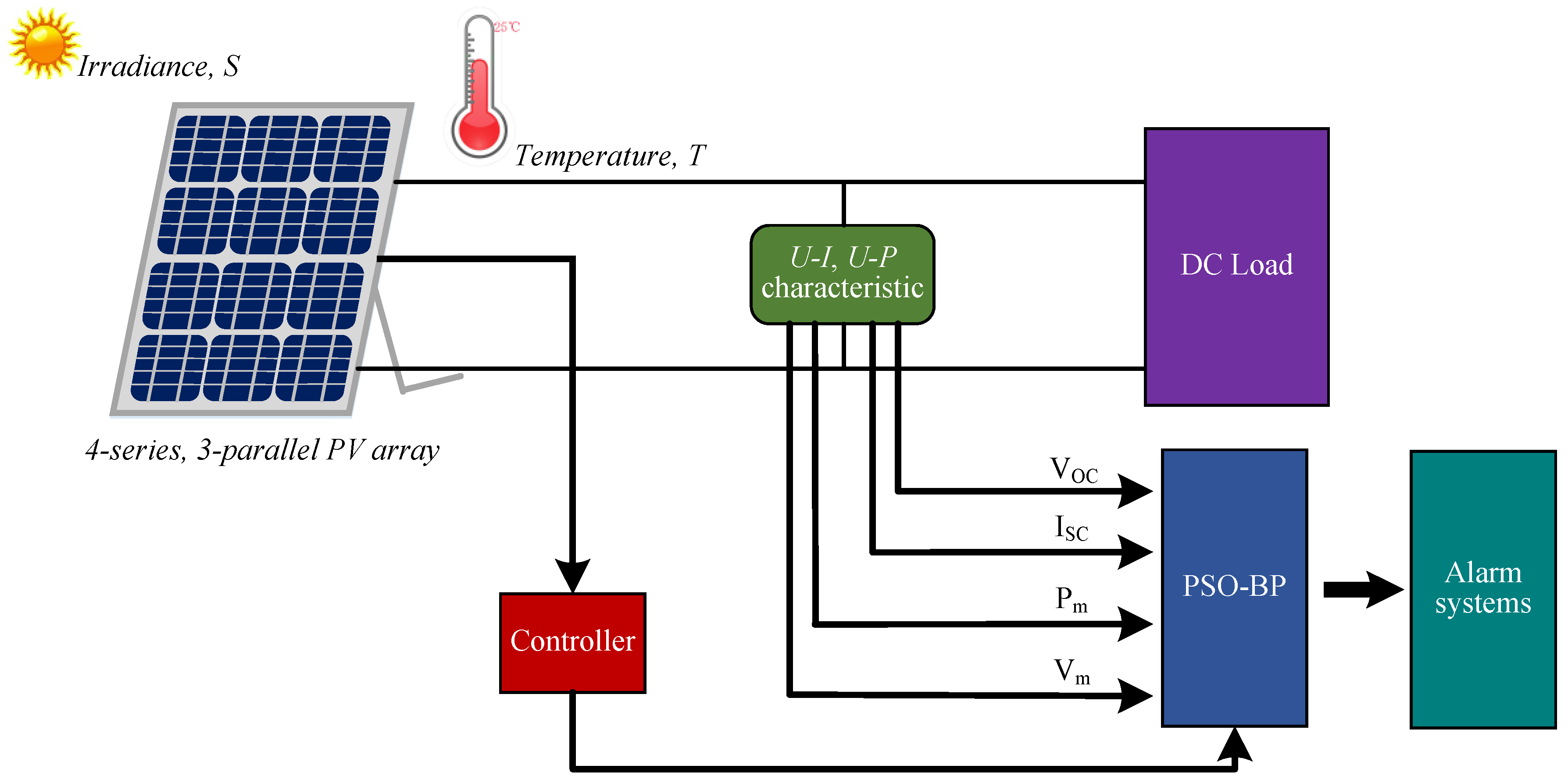
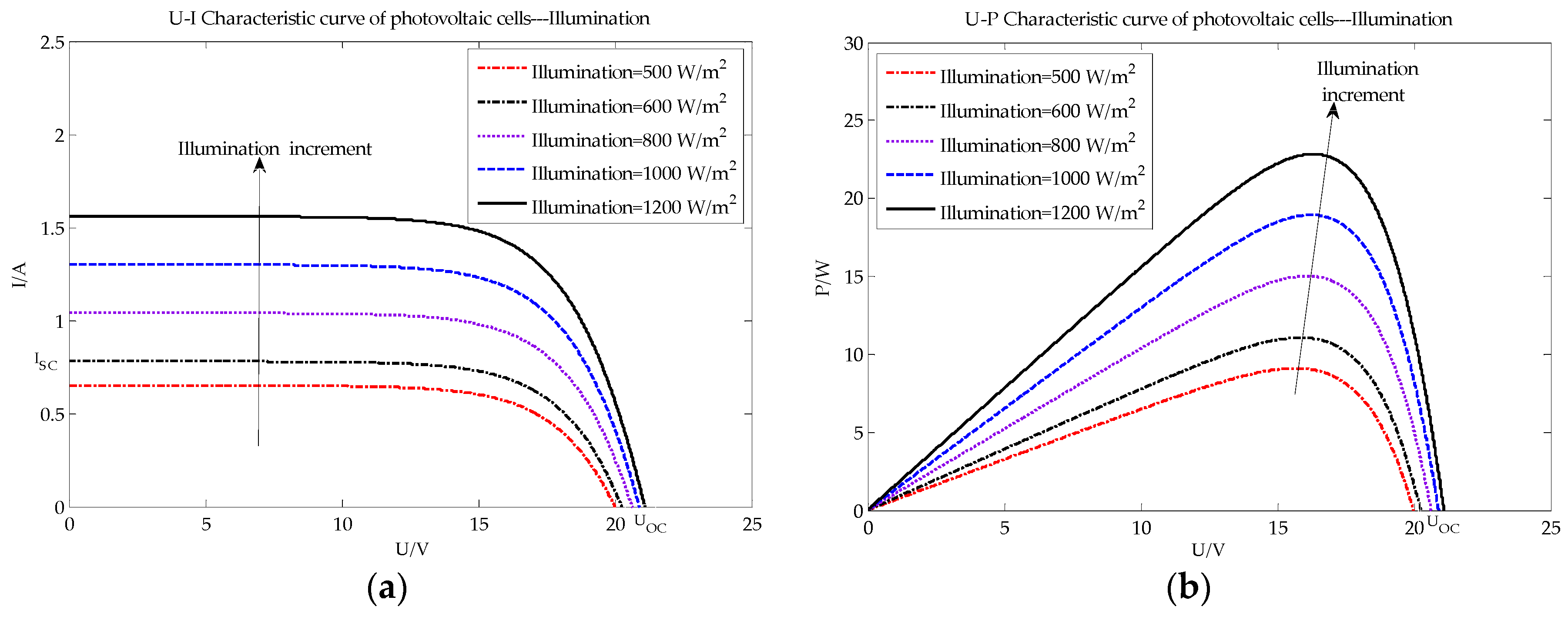
We analyze the performance of PVs under various fault conditions, using open-circuit voltage (V_oc), short-circuit current (I_sc), maximum power (P_m) and voltage at maximum power point (V_m) to construct feature recognition criteria. The criteria reduce the running space and shorten the program execution time of the heuristic diagnostic method.

(2)

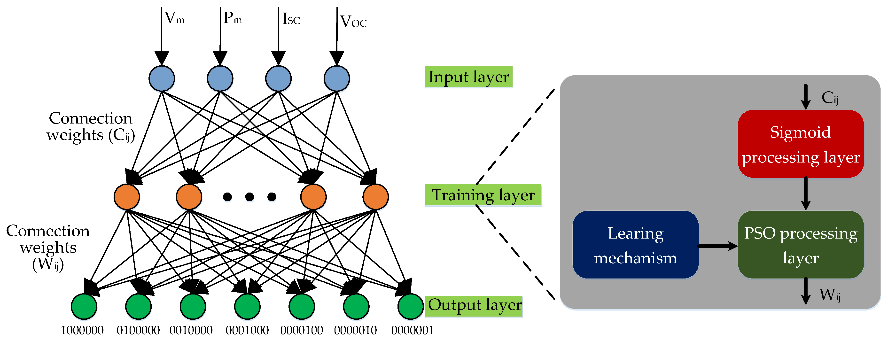
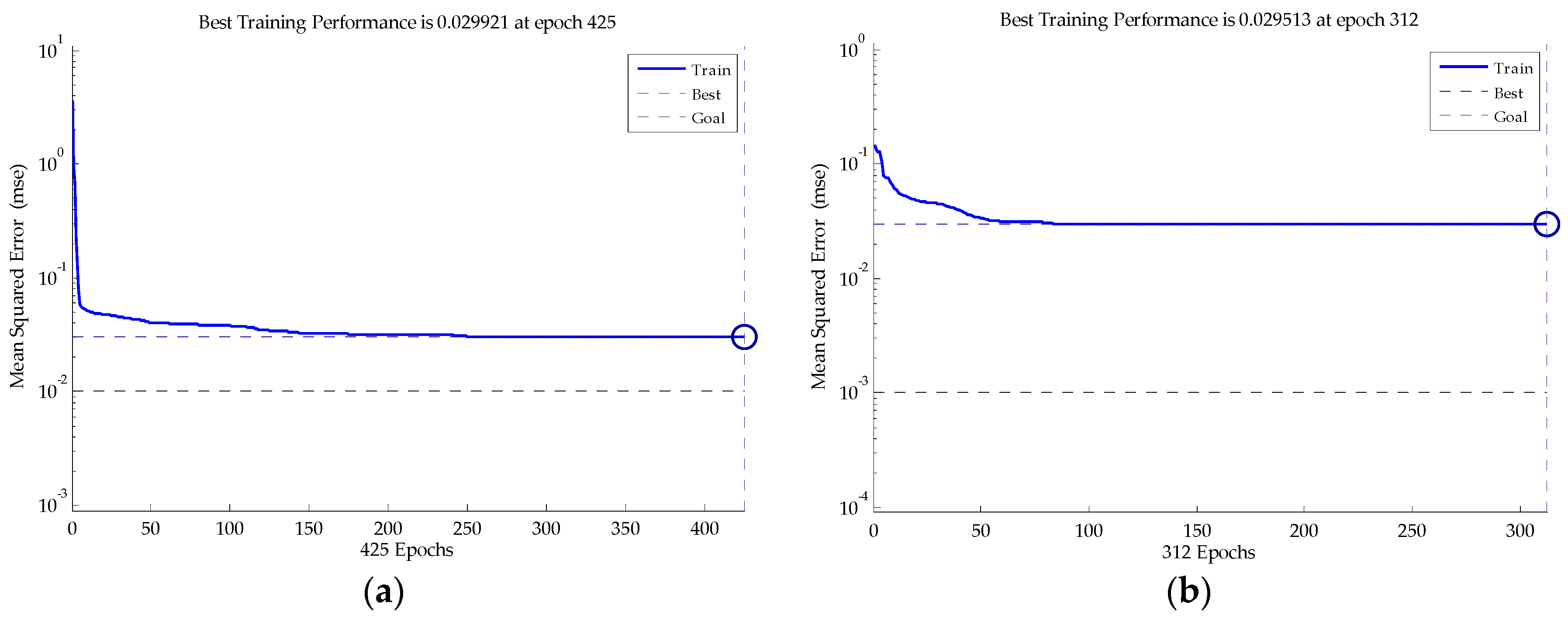
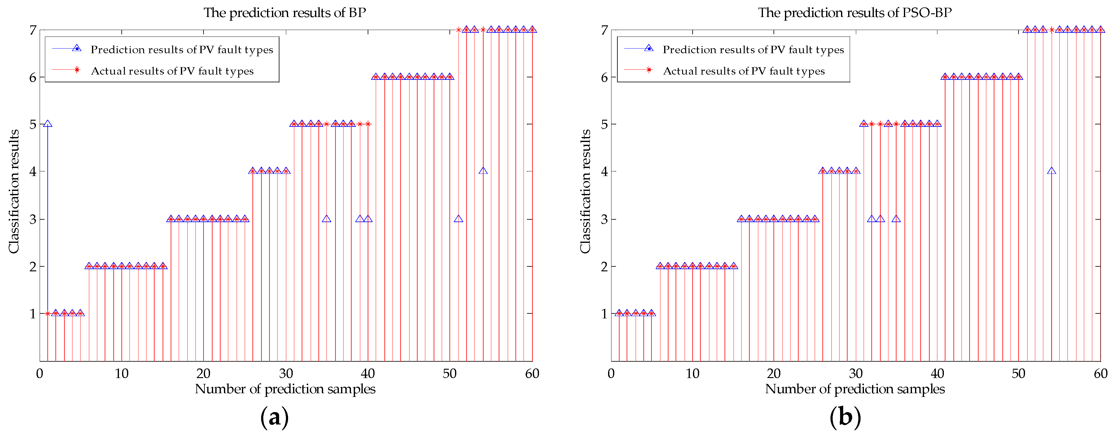
We evaluate the performance of a heuristic particle swarm optimization–back-propagation (PSO-BP) neural network method applied in PV fault diagnosis. The method has the merits of global search ability for particle swarm optimization (PSO) and local search ability for BP. The PSO-BP neural network ameliorates the convergence of the diagnostic method and improves the prediction accuracy of the photovoltaic diagnosis system effectively.

The remainder of this paper is organized as follows. Section 2 describes the fault diagnosis system used in this study and the fault recognition parameters. Section 3 presents our proposed approach: a triple-layered PSO-BP neural network for forecasting faults in PV systems. Section 4 describes the data used in this study. Fault recognition and predictions using PSO-BP are examined with MATLAB in Section 5. Section 6 concludes the paper.

2. Configuration of Proposed System

The schematic diagram of our proposed fault diagnosis system is shown in Figure 1. It is mainly composed of a 4 × 3 (4 in series, 3 in parallel) PV array module, with DC load, alarm systems, and data processing modules acquiring and recording the state of the PV system. A triple-layered heuristic PSO-BP neural network is used as the diagnostic tool.

In order to analyze changing of PV parameters in different fault conditions, a PV module simulation platform based on MATLAB/Simulink was used in this paper, in accordance with the mathematical model in [14]. The specification of this module under a standard test condition (STC) is presented in

Table 1. Electrical parameters of photovoltaic (PV) modules under standard test condition (STC): AM (Air-Mass) = 1.5, irradiance = 1000 W/m², temperature = 300 K.

Electrical Parameters	Value (Unit)
Maximum power	21 (W)
Open-circuit voltage	21.7 (V)
Short-circuit current	1.3 (A)
Voltage at maximum power point	17.6 (V)
Current at maximum power point	1.17 (A)

.

The simulation was carried out under different fault conditions, including temperature faults, partial shade faults, and faults due to aging cells (different series resistances imply differently aging cells [15]). I-U and voltage-power (U-P) characteristic curves were produced, as shown in Figure 2, Figure 3 and Figure 4, respectively.

With the increase of the cell’s temperature, as seen in Figure 2, I_sc increases while the V_oc, P_m and V_m decrease. The main causes of these changes are as follows: the bandgap is negatively correlated with the ambient temperature; with increasing ambient temperature, the Fermi energy of the PV gradually approaches the center of the forbidden band; and the PV diffusion coefficient is positively correlated with the I_sc and Fermi energy.

As Figure 3 shows, due to the PV effect, the photons exceeding the PV cells’ bandgap excite a large number of electron hole pairs, which then generate electromotive force and current. Therefore, with increasing illumination of the PV cells, the I_sc, V_oc, P_m and V_m increase.

Figure 4 graphs the PV array with different series resistances. As the series resistance decreases I_sc and V_oc have minor changes, while P_m and V_m increase.

These results indicate that V_oc, I_sc, P_m and V_m can be used to determine whether there is a fault in the PV array, as well as the corresponding cause of the fault. Here, V_oc, I_sc, P_m and V_m are used as identification parameters for the PV fault diagnosis system, and are expressed as an input matrix $X$.

$$X=\left[{\mathrm{V}}_{oc}{I}_{sc}{\mathrm{P}}_m{\mathrm{V}}_m\right].$$

(1)

3. Proposed Fault Diagnosis Method

The PSO-BP neural network is a model combining features of the global search ability of PSO with the local search ability of a BP neural network [16]. In order to get the solution of PSO quickly, a heuristic model of the PSO-BP neural network is used in this paper to predict the faults of the PV array. In our model, the test data are normalized and delivered to the benchmark input layer, and are subsequently trained and proceed with a sigmoid function in the benchmark training layer, on which the classification and learning mechanism are built. In practice, the recorded real-time fault data of the PV system proceed in the same way and are imported into the PSO processing layer to optimize fault classification. The results of the optimization are obtained in the output layer. The schematic diagram of the triple-layered heuristic diagnostic method is shown in Figure 5.

(1) Normalize the different magnitudes of the recorded fault characteristics

Owing to the different units and magnitudes of V_oc, I_sc, P_m and V_m, we normalize the input matrix $X$ by the linear transformation method [17]:

$$z_{ij}=\left(x_{ij}-x_{\min }\right)\cdot \frac{y_{\max }-y_{\min }}{x_{\max }-x_{\min }}+y_{\min }$$

(2)

where $x_{ij}$ and $z_{ij}$ are the initial and normalized input matrices, $x_{\min }$ and $x_{\max }$ are the minimum and maximum values of each row of $X$ respectively, and $y_{\min }$ and $y_{\max }$ are the minimum and maximum values of each row in the normalized matrix. In this paper $y_{\min }=-1$, $y_{\max }=1$.

(2) Encode the fault states of the PV fault diagnosis system

To verify the feasibility of the PV fault diagnosis system, this paper investigates seven kinds of PV faults and encodes them by 0 and 1 for identification purposes, as shown in

Table 2. The operative states of the PV array and its corresponding 0–1 coding matrix.

Fault States	States Code	0–1 Code
Normal	1	1000000
Temperature fault	2	0100000
Partial fading fault	3	0010000
Cells aging	4	0001000
Combination of temperature and partial shade faults	5	0000100
Combination of temperature fault and cells aging	6	0000010
Combination of partial shade fault and cells aging	7	0000001

.

(3) Process the normalized fault characteristics using sigmoid function, and select the optimal results as the multi-dimensional search space of PSO

A suitable number of neurons in the hidden-layer and activation functions are conducive for the PSO-BP neural network to quickly and effectively complete the training with less training times and higher convergence rates [18,19].

The sigmoid function is expressed as

$$S\mathrm{ig}\left(\mathrm{x}\right)=\frac{1}{1+e^{-\alpha \mathrm{x}}}.$$

(3)

The linear function is expressed as

$$Linear\left(\mathrm{x}\right)=k\cdot \mathrm{x}+c.$$

(4)

The required number of hidden neurons of the BP neural network is calculated by the following formula [9,20]:

$$n=floor\left(\sqrt{n_i+n_o}+a\right)$$

(5)

where $floor(\times )$ is a round-down function, such as $floor\left(1.2\right)=1$, $n$ is the number of neurons in the hidden layer, $n_i$ is the number of neurons in the input layer, $n_o$ is the number of neurons in the output layer, and $a$ is an empirical constant.

The connection weight $C_{ij}$ connects neuron i of the hidden layer and neuron j of the input layer of the BP neural network by the sigmoid function, while the connection weight ${\mathrm{W}}_{ij}$ connects the output layer and the hidden layer by the linear function. The training deviation and epochs corresponding to the neurons are illustrated in Figure 6. The line with red dots indicates the number of epochs when the BP neural network is trained by increasing the neurons of the hidden layer, while the line with black squares illustrates the training accuracy of the BP neural network with the increase of the hidden layer neurons. As shown in Figure 6, when the number of neurons in the hidden layer is 12, the training accuracy of the BP neural network is over 80%, and the number of epochs is about 100 steps.

The expression of the output matrix that is transmitted from the input layer to the output layer via the hidden layers is as follows:

$$Z_{out}=\mathrm{Sig}\left(Z_{in}{C}^T\right)$$

(6)

$$P_{in}=Z_{out}$$

(7)

$$P_{out}=f_1\left(P_{in}\right)$$

(8)

$$L_{in}=P_{out}$$

(9)

$$L_{out}=Linear\left(L_{in}{W}^T\right)$$

(10)

where $Z_{in}$ is a normalized input matrix, $Z_{in}=[z_{xy}]$, $Z_{out}$ is the output matrix processed by transposed matrix $C^T$ and sigmoid function between the input layer and the sigmoid processing layer; $P_{in}$ is the input matrix from the sigmoid processing layer to the PSO processing layer, $P_{out}$ is the output matrix optimized by PSO, $f_1$ is the PSO processing method, $L_{in}$ is the input matrix from the PSO processing layer to the output layer, and $L_{out}$ is the output matrix processed by transposed matrix $W^T$ and the linear function between the PSO processing layer and output layer.

(4) Update the position and velocity of the particles processed by sigmoid function, and the parameters in PSO

In the PSO method, the optimal training results are selected as the initial N-dimensional search space. The particles processed by the sigmoid function start from the initial position $S_i$ with the velocity $V_i$. The initial best position of the particles is set as $pbes{t}_0$, and the initial best position of the whole swarm is set as $gbes{t}_0$ [21].

In the updating phase, supposing pbest and gbest of the i-th particle in N-dimensional space are $P_i=\left(p_{i1},p_{i2},\cdots ,p_{iN}\right)$ and $G_i=\left(g_{i1},g_{i2},\cdots ,g_{iN}\right)$, the updating rule of the particle’s position $s_{i\cdot n}$ and velocity $v_{i\cdot n}$ is given by following equation series [22,23,24]:

$$v_{i\cdot n}\left(t+1\right)=\omega v_{i\cdot n}\left(t\right)+c_1{r}_1\left[p_{i\cdot n}\left(t\right)-s_{i\cdot n}\left(t\right)\right]+c_2{r}_2\left[g_{i\cdot n}\left(t\right)-s_{i\cdot n}\left(t\right)\right]$$

(11)

$$s_{i\cdot n}\left(t+1\right)=s_{i\cdot n}\left(t\right)+a\cdot v_{i\cdot n}\left(t+1\right)$$

(12)

$$\omega ={\omega }_{\max }-\frac{{\omega }_{\max }-{\omega }_{\min }}{T_{\max }}\cdot t$$

(13)

$$v_{i\cdot n}\left(t\right)=\{\begin{array}{l}{v}_{\max },v_{i\cdot n}\left(t\right)>v_{\max }\\ -v_{\max },v_{i\cdot n}\left(t\right)<-v_{\max }\end{array}$$

(14)

where ${\omega }_{\min }\le \omega \le {\omega }_{\max }$ is defined as inertia weight factor. When $\omega \to {\omega }_{\max }$ the particle has stronger global searching ability, has a bigger search space, and can find a new solution domain. However, higher values of $\omega$ may skip the optimal solution domain. While $\omega \to 0$, the particle has stronger searching ability locally, which is beneficial to obtain the optimal solution of the particle in the solution space, but the search time will be accordingly long. $0<t\le T_{\max }$ is the iteration time. $c_1$ and $c_2$ are constants for the cognitive factor and social factor, respectively. When $c_1=0$, the particle does not have cognitive ability and lacks local search, the particle has the ability to expand the search space, and the PSO is known as a social-only model, which has faster convergence and global optimization capability, but falls more easily into the local optimum. When $c_2=0$, there is no interaction between the particles in the particle swarm, and the PSO is known as a cognition-only model. Because the particles moves blindly, the model easily leads the convergence slowly, and it is difficult to obtain the global optimal solution [24,25]. Independent random numbers $r_1$ and $r_2$ are uniformly distributed in the range of [0, 1]. $v_{i\cdot n}\in \left\{-v_{\max },v_{\max }\right\}$, where $v_{\max }$ is the maximum particle velocity, $p_{i\cdot n}\left(t\right)$ is the best previous position of particle i along the n-th dimension in iteration t, $g_{i\cdot n}\left(t\right)$ is the best previous position among all the particles along the n-th dimension in iteration t, and $a$ is the constraint factor, $a=1$.

(5) Calculate and evaluate the particles’ fitness in the particle swarm

To calculate the particles’ initial fitness in the PSO method, take the mean square error of the network as the fitness function, the current position of the particle as the particle’s own best position, and the current position of the particle swarm as the initial particle swarm best position. The mean square error is defined as follows:

$$MS{E}_j=\frac{1}{2}{\displaystyle \sum _{i=1}^N{\left(y_{ij\cdot rel}-y_{ij\cdot out}\right)}^2}$$

(15)

where j is the fault states code of PV system, $j=1,2,\cdots ,7$. $MS{E}_j$ is the error for the j-th pattern vector, $y_{ij\cdot rel}$ the desired value of the output, and $y_{ij\cdot out}$ the actual output of the j-th output neuron.

If the new particle position is better than the current pbest, update the particle’s new position with the latest pbest. If the particle swarm’s new position is better than gbest, update the particle swarm’s new position with the latest gbest.

(6) Judge whether the maximum iterations are achieved or the training error is less than the prescribed standard error in PSO

If the maximum iterations are achieved or the training error is less than the prescribed standard error, search for the best position of the particle swarm in the vicinity of the current gbest using the BP neural network; if the search result is better than the current gbest, then output the search result. Otherwise, output the current gbest to obtain the optimized neural network, or go back to step 3, until the requirements of the fault diagnosis method are met.

4. Data Collection

To verify the reliability of the PV array model built in MATLAB/Simulink (R2012a, MathWorks, Natick, MA, USA), simulation was performed under the standard conditions. 210 set of the values of V_oc, I_sc, P_m and V_m when $Illumination\in \left[100\mathrm{W}/m^2,2000\mathrm{W}/m^2\right]$, $Temperature\in \left[273.15\mathrm{K},373.15\mathrm{K}\right]$ and the series resistance of cells $R_s\in \left[0.5\Omega ,5.5\Omega \right]$ are used as the data sample of the PSO-BP neural network, 150 sets were used as the training sample for the PSO-BP neural network, and the remaining 60 sets were used as the test sample. The values used for important parameters of the PSO-BP neural network are shown in

Table 3. Some important parameters in the PSO-BP neural network.

Parameters (Symbol)	Value	Parameters (Symbol)	Value
Population (M)	40	Cognitive factor ($c_1$)	2
Maximum iteration ($T_{\max }$)	200	Social factor ($c_2$)	3
Maximum inertia weight (${\omega }_{\max }$)	1.8	Maximum particle velocity ($v_{\max }$)	0.05
Minimum inertia weight (${\omega }_{\min }$)	1.7

.

5. Results and Analysis

The collected data were introduced to the BP neural network proposed in [9,11] and the PSO-BP neural network proposed in this paper and analyzed by MATLAB. The training mean squared error based on 150 training samples and the prediction results of the 60 test samples in the fault diagnosis system, are shown in Figure 7 and Figure 8.

As can be seen from Figure 7, in the training phase, the BP neural network method takes about 425 steps to achieve convergence, while the heuristic PSO-BP method only needs 312 steps. The mean squared error of the heuristic method is also smaller than that of the BP neural network method. The heuristic PSO-BP neural network method gives a quick and effective optimization training process, and ensures that the fault diagnosis system has greater accuracy.

In Figure 8, it is shown that for the 60 test samples in the fault diagnosis system, there are six misprediction points and the predictive accuracy is only 86.67% with the BP neural network method, while there are only four misprediction points with the heuristic method, which has predictive accuracy of 93.33%. Therefore, the heuristic PSO-BP neural network method can be used to more accurately predict fault type in a PV array.

In order to compare the advantages and disadvantages of the two algorithms, we selected 10 set of typical data from the test samples. The results are shown in

Table 4. Prediction accuracy comparison for the two algorithms.

Sample	Content				Actual Fault Code	Predict Result		Right or Wrong 1
	Voc (V)	Isc (A)	Pm (W)	Vm (V)		BP	PSO-BP	BP	PSO-BP
1	20.9756	1.2943	18.9784	16.3230	1000000	0000100	1000000	×	√
2	21.0542	1.2903	19.0131	16.3905	1000000	1000000	1000000	√	√
3	16.4707	1.5209	16.1174	12.2254	0100000	0100000	0100000	√	√
4	18.8417	0.3103	4.0822	14.7464	0010000	0010000	0010000	√	√
5	20.8974	1.2976	14.3561	13.2862	0001000	0001000	0001000	√	√
6	20.2456	0.7783	11.0650	15.8445	0000100	0010000	0010000	×	×
7	21.0960	1.0863	16.1384	16.5977	0000100	0010000	0000100	×	√
8	21.1328	1.2863	18.9137	16.3732	0000010	0000010	0000010	√	√
9	21.2950	1.9482	28.3066	16.2328	0000001	0010000	0000001	×	√
10	20.8974	1.2981	17.3409	15.1531	0000001	0001000	0001000	×	×

¹ The final two columns indicate whether the prediction results are correct or wrong using the BP neural network method and the PSO-BP neural network method; “√” means the prediction result is correct; “×” means the prediction result is wrong.

.

6. Conclusions

Based on the analysis of the output characteristics of the PV system, V_oc, I_sc, P_m, and V_m were extracted as the identification parameters for the fault diagnosis system. The PSO-BP neural network method was applied to improve the fault diagnosis system and predict fault type for 60 test samples of six typical fault types, including PV temperature fault, partial shade fault, aging cells, the combination of temperature and shade, the combination of temperature fault and aging cells, and the combination of shading and aging cells. Simulation results show that the heuristic PSO-BP neural network method not only improves the convergence of the prediction algorithm, but also significantly augments the prediction accuracy of the fault diagnosis system. Furthermore, the intelligent algorithm used in this paper can predict the fault type in real time without additional hardware support.

Owing to the complexity and uncertainty of the fault information of PV system, the method proposed in this paper needs to be further studied in the future for on-line diagnosis of more fault types.

References

1. Masson, G.; IEA PVPS Task 1. 2015 Snapshot of Global Photovoltaic Markets; IEA Photovoltaic Power Systems Programme: St. Ursen, Switzerland, 2016; pp. 4–10. [Google Scholar]
2. Singh, P.; Ravindra, N.M. Temperature dependence of solar cell performance—An analysis. Sol. Energy Mater. Sol. Cells 2012, 101, 36–45. [Google Scholar] [CrossRef]
3. Bai, J.B.; Cao, Y.; Hao, Y.Z.; Zhang, Z.; Liu, S.; Cao, F. Characteristic output of PV systems under partial shading or mismatch conditions. Sol. Energy 2015, 112, 41–54. [Google Scholar] [CrossRef]
4. Kaushika, N.D.; Rai, A.K. An investigation of mismatch losses in solar photovoltaic cell networks. Energy 2007, 32, 755–759. [Google Scholar] [CrossRef]
5. Takashima, T.; Yamaguchi, J.; Otani, K.; Kato, K.; Ishida, M. Experimental studies of failure detection methods in PV module strings. In Proceedings of the IEEE 4th World Conference on Photovoltaic Energy Conversion, Waikoloa, HI, USA, 7–12 May 2006; pp. 2227–2230.
6. Takashima, T.; Yamaguchi, J.; Ishida, M. Disconnection detection using earth capacitance measurement in photovoltaic module string. Prog. Photovolt. 2008, 16, 669–677. [Google Scholar] [CrossRef]
7. Chao, K.H.; Chen, P.Y.; Wang, M.H.; Chen, C.T. An intelligent fault detection method of a photovoltaic module array using wireless sensor networks. Int. J. Distrib. Sens. Netw. 2014, 2014, 1–12. [Google Scholar] [CrossRef]
8. Hsieh, C.T.; Shiu, J. Study of intelligent photovoltaic system fault diagnostic scheme based on chaotic signal synchronization. Math. Probl. Eng. 2013, 2013, 816296. [Google Scholar] [CrossRef]
9. Wang, Y.Z.; Li, Z.H.; Wu, C.H.; Zhou, D.Q.; Fu, L. A survey of fault diagnosis for PV array based on BP neural network. Power Syst. Prot. Control 2013, 41, 108–114. [Google Scholar]
10. Wu, Y.C.; Lan, Q.L.; Sun, Y.Q. Application of BP neural network fault diagnosis in solar photovoltaic system. In Proceedings of the IEEE International Conference on Mechatronics and Automation, Changchun, China, 9–12 August 2009; pp. 2581–2585.
11. Mellit, A.; Kalogirou, S.A. Artificial intelligence techniques for photovoltaic applications: A review. Prog. Energy Combust. 2008, 34, 574–632. [Google Scholar] [CrossRef]
12. Mas’ud, A.A.; Albarracín, R.; Ardila-Rey, J.A.; Muhammad-Sukki, F.; Illias, H.A.; Bani, N.A.; Munir, A.B. Artificial Neural Network Application for Partial Discharge Recognition: Survey and Future Directions. Energies 2016, 9, 574. [Google Scholar] [CrossRef]
13. Rumelhart, D.E.; Hinton, G.E.; Williams, R.J. Learning internal representations by error propagation. In Parallel Distributed Processing: Exploration in the Microstructure of Cognition, 1st ed.; MIT Press: Cambridge, MA, USA, 1986; pp. 318–362. [Google Scholar]
14. Singh, P.; Singh, S.N.; Lal, M.; Husain, M. Temperature dependence of I–V characteristics and performance parameters of silicon solar cell. Sol. Energy Mater. Sol. Cells 2008, 92, 1611–1616. [Google Scholar] [CrossRef]
15. Meyer, E.; Dyk, E.E.V. Assessing the reliability and degradation of photovoltaic module performance parameters. IEEE Trans. Reliab. 2004, 53, 83–92. [Google Scholar] [CrossRef]
16. Zhang, J.R.; Zhang, J.; Lok, T.M.; Lyu, M.R. A hybrid particle swarm optimization–back-propagation algorithm for feedforward neural network training. Appl. Math. Comput. 2007, 185, 1026–1037. [Google Scholar] [CrossRef]
17. Khadse, C.B.; Chaudhari, M.A.; Borghate, V.B. Conjugate gradient back-propagation based artificial neural network for real time power quality assessment. Int. J. Electr. Power 2016, 82, 197–296. [Google Scholar] [CrossRef]
18. Dasgupta, B.; Schnitger, G. The power of approximating: A comparison of activation functions. In Advances in Neural Information Processing Systems; Giles, C.L., Hanson, S.J., Cowan, J.D., Eds.; Morgan Kaufmann Publishers Inc.: Burlington, VT, USA, 1993; pp. 615–622. [Google Scholar]
19. Ismail, A.; Jeng, D.-S.; Zhang, L.L.; Zhang, J.-S. Predictions of bridge scour: Application of a feed-forward neural network with an adaptive activation function. Eng. Appl. Artif. Intell. 2013, 26, 1540–1549. [Google Scholar] [CrossRef]
20. Xu, C.Y.; Xu, C.F. Optimization analysis of dynamic sample number and hidden layer node number based on BP neural network. In Proceedings of the Eighth International Conference on Bio-Inspired Computing: Theories and Applications, Hefei, China, 12–14 July 2013.
21. Li, J.Y.; Shi, J.F.; Li, J.C. Exploring Reduction Potential of Carbon Intensity Based on Back Propagation Neural Network and Scenario Analysis: A Case of Beijing, China. Energies 2016, 9, 615. [Google Scholar] [CrossRef]
22. Moradi, M.H.; Abedini, M. A combination of genetic algorithm and particle swarm optimization for optimal DG location and sizing in distribution systems. Int. J. Electr. Power 2012, 34, 66–74. [Google Scholar] [CrossRef]
23. Wang, G.G.; Gandomi, A.H.; Yang, X.S.; Alavi, A.H. A novel improved accelerated particle swarm optimization algorithm for global numerical optimization. Eng. Comput. 2014, 31, 1198–1220. [Google Scholar] [CrossRef]
24. Khare, A.; Rangnekar, S. A review of particle swarm optimization and its applications in Solar Photovoltaic system. Appl. Soft Comput. 2013, 13, 2997–3006. [Google Scholar] [CrossRef]
25. Ratnaweera, A.; Halgamuge, S.K.; Watson, H.C. Self-organizing hierarchical particle swarm optimizer with time-varying acceleration coefficients. IEEE Trans. Evolut. Comput. 2004, 8, 240–255. [Google Scholar] [CrossRef]
Figure 1. Schematic diagram of the fault diagnosis system.
Energies 10 00226 g001
Figure 2. PV characteristic curve under different temperature conditions: (a) U-I characteristic curve of PV array; (b) U-P characteristic curve of PV array.
Energies 10 00226 g002
Figure 3. PV characteristic curve under different illumination conditions: (a) U-I characteristic curve of PV array; (b) U-P characteristic curve of PV array.
Energies 10 00226 g003
Figure 4. PV characteristic curve under different series resistance conditions: (a) U-I characteristic curve of PV array; (b) U-P characteristic curve of PV array.
Energies 10 00226 g004
Figure 5. Schematic diagram of the triple-layered heuristic PSO-BP neural network method.
Energies 10 00226 g005
Figure 6. The training deviation and epochs corresponding to the neurons.
Energies 10 00226 g006
Figure 7. The training mean squared error in two methods. The blue solid line is the mean squared error in the training process, while the dot line is the target mean squared error in the MATLAB. (a) The training mean squared error of the BP neural network; (b) the training mean squared error of the PSO-BP neural network.
Energies 10 00226 g007
Figure 8. The prediction results for the two methods. The blue triangles are the prediction results of the two diagnostic methods, and the red asterisks are the actual fault classifications of the 60 test samples. (a) The prediction results of the BP neural network; (b) the prediction results of the PSO-BP neural network.
Energies 10 00226 g008