Exploring the Environment/Energy Pareto Optimal Front of an Office Room Using Computational Fluid Dynamics-Based Interactive Optimization Method

Abstract

This paper is concerned with the development of a high-resolution and control-friendly optimization framework in enclosed environments that helps improve thermal comfort, indoor air quality (IAQ), and energy costs of heating, ventilation and air conditioning (HVAC) system simultaneously. A computational fluid dynamics (CFD)-based optimization method which couples algorithms implemented in Matlab with CFD simulation is proposed. The key part of this method is a data interactive mechanism which efficiently passes parameters between CFD simulations and optimization functions. A two-person office room is modeled for the numerical optimization. The multi-objective evolutionary algorithm—non-dominated-and-crowding Sorting Genetic Algorithm II (NSGA-II)—is realized to explore the environment/energy Pareto front of the enclosed space. Performance analysis will demonstrate the effectiveness of the presented optimization method.

1. Introduction

Over the past two decades, the energy consumption in buildings accounted for 20–40% of the total worldwide energy consumption [1]. In China, buildings consumed 756 million tons of standard coal, accounting for 19.5% of the total national energy consumption in 2013 [2]. Even with such high energy consumption, the resulting indoor environments are not satisfactory. According to survey data from the International Facility Management Association [3], poor thermal comfort and poor indoor air quality (IAQ) are still the predominant complaints of office occupants.

Various optimization strategies have grown in popularity due to increasing concerns on the thermal comfort, IAQ, and building energy consumption simultaneously. For stratified or partially mixed air distribution systems, it is important to take spatial influence into consideration. Such optimization strategies require the knowledge of various distributed environmental parameters, such as air temperature, air velocity, and contaminant concentrations. Recently, computational fluid dynamics (CFD) combined with optimization algorithms has been the most popular method for optimizing the performance of enclosed spaces. These methods mainly include CFD-based parametric studies, CFD-based data-driven methods, and CFD-coupled optimization algorithms.

Many researchers employed parametric studies [4,5,6] to achieve better performance of enclosed environments. In the parametric studies, one usually fixes all but one variable, and tries to optimize a cost function with respect to the non-fixed variable. Every time a variable is varied, all other variables typically become non-optimal, and hence also need to be adjusted. Such a manual procedure is very time-consuming using CFD simulations, and is often impractical for more than two or three independent variables. Researchers [7,8,9,10,11] also combined data-driven methods with CFD to relieve computing burden. Zhou and Haghighat [7,8] applied artificial neural networks (ANNs) in place of CFD simulation inside genetic algorithm (GA) search loops to improve thermal comfort and IAQ without sacrificing energy costs of ventilation systems in office buildings. The proper orthogonal decomposition (POD) method is a reduced-order method that can also be applied in CFD-based optimization design. Li et al. [10] integrated the POD model of thermo-fluid flow into GA to optimize the air-supply velocity and temperature efficiently. While the data-driven results are encouraging, the model accuracy and generalization capabilities limit their applications.

With respect to CFD-coupled optimization algorithms, Kim et al. [12] established a two-step method for optimal design of the indoor thermal environment. In the first step, the GA search used a simplified simulation with one-point model presuming the perfect mixing of air temperature and humidity. In the second step, detailed CFD simulations were conducted for investigation of the optimal design candidates. Lee [5] also designed a similar two-step method for optimization of indoor climate conditions considering passive and active variables such as climatic conditions. More control-friendly and accurate optimization frameworks are frequently reported in the field of building enclosure design. Commercial optimization packages such as GenOpt, BeOpt, and Opt-E-Plus have been successfully applied in various practical optimizations [13,14,15,16]. Futrell et al. [16] combined Genopt with EnergyPlus to find efficient solutions to the daylighting and thermal performance of a classroom design. Asadi et al. [15] employed TRNSYS and GenOpt to optimize the retrofit cost, energy savings, and thermal comfort of a residential building. However, when the model file was considerably large—which is the general situation for partial differential equation (PDE) related indoor environmental simulation—they became inefficient or even crashed. Of the few papers in the literature that give detailed descriptions of the tools used to combine CFD simulation with optimization algorithm, most require modification and adaptation of existing optimization algorithms. Liu et al. [17,18] used the CFD solver OpenFOAM [19] to establish an adjoint system for the optimal design of indoor environmental parameters. A steepest descent method and GA were implemented, respectively, in the C++-based OpenFOAM.

In this paper, a CFD-coupled optimization method is proposed for finding the environment/ energy Pareto front of an enclosed environment simultaneously. An efficient and control-friendly optimization scheme is developed which can facilitate optimization designs with existing simulation tools and standard Matlab-based algorithms. The key part of this method is a data interactive mechanism which links CFD simulation to Matlab, which means that plenty of optimization algorithms can be conveniently used without requiring code adaptation. On this basis, a validated model of an office room equipped with a thermal displacement ventilation system (TDVS) is established. Additionally, a kind of multi-objective optimization algorithm—non-dominated-and-crowding Sorting Genetic Algorithm II (NSGA-II)—is applied to explore the Pareto optimal front of occupied zones’ thermal comfort, IAQ, and energy cost of heating, ventilation and air conditioning (HVAC) system. Performance investigations will show the effectiveness of the proposed optimization framework.

The rest of the paper is organized as follows. Section 2 depicts the optimization framework based on data interactive mechanism. An optimization case using the proposed framework is investigated in Section 3. Section 4 provides the application results and analysis. Some concluding remarks and future works are given in Section 5.

2. Optimization Framework

2.1. Problem Description

To optimize the performance of enclosed spaces, CFD-coupled optimization methods are proven to be more efficient than other approaches. The designers still lack optimization tools for conveniently combining CFD simulation and optimization algorithms. We begin by looking at the optimization problem definition, then describe the framework developed to address it.

Consider an optimization problem of the form:

$${\mathbf{P}}_{\mathbf{c}}:\underset{x\in \mathbf{X}}{\min }f\left(x\right)$$

(1)

where $f:{\mathbb{R}}^n\to \mathbb{R}$, X is a user-specified constraint set. We here discuss problem ${\mathbf{P}}_{\mathbf{c}}$ for the situation where the objective function f may not be solved directly, but can be approximated numerically by approximating functions $f^{*}:{\mathbb{R}}_{+}^p\times {\mathbb{R}}^n\to \mathbb{R}$, where the first argument is the precision parameter of the numerical solvers. This is generally the case when the objective function is evaluated by a CFD-related simulation, such as Fluent, Airpak, Comsol, etc.

In such simulations, computing the objective function involves solving Navier–Stokes equations that are coupled to other partial/ordinary differential equations or algebraic equations. In general, one can only obtain an approximate numerical solution instead of an exact one. Hence, the objective function $f\left(x\right)$ can only be approximated by an approximating function $f^{*}(\epsilon ,x)$, where $\epsilon \in {\mathbb{R}}_{+}^p$ is a vector that contains precision parameters of the numerical solvers. Consequently, the optimization algorithm may only be applied to $f^{*}(\epsilon ,x)$.

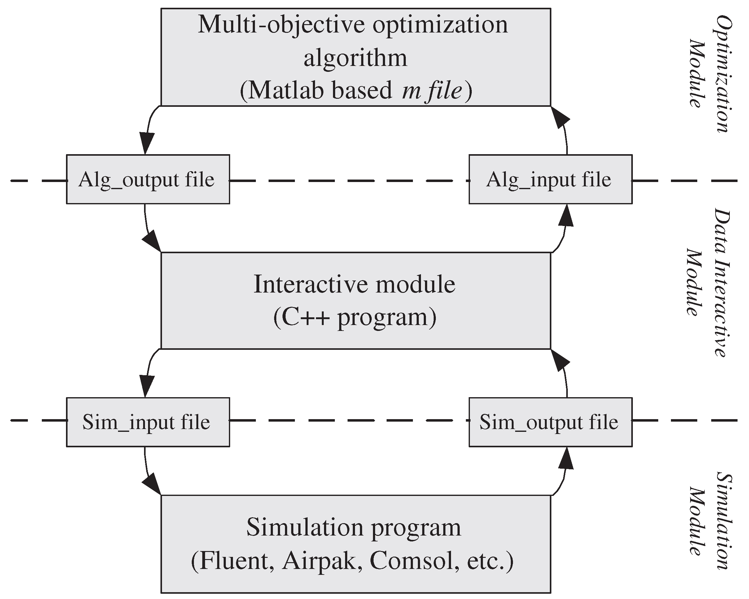
2.2. Data Interactive Mechanism-Based Optimization Strategy

The general optimization framework is described in Figure 1. Within the framework, the problem is divided into three modules: the simulation module consists of any standard simulation program, such as Fluent, Airpak, Comsol, etc.; the optimization module is designed using Matlab, in which various single/multiple-objective optimization algorithms are realized; the data interactive module is constructed by a C++ program, which is used to couple CFD simulation with Matlab-based optimization algorithms without requiring code adaptation.

The data interactive module plays the key role of the proposed optimization strategy. It interfaces with two commercially available computer programs, with no need for source code modifications or complex connections between programs. Text type files (Figure 1) are used for data exchange between the two modules. For each iteration, the data interactive module works as the following scheme:

Start

Read control variables from $Alg\_outputfile$

Delete old $Sim\_inputfile$ of CFD simulation (for Fluent, it is *.cas)

Create a new $Sim\_inputfile$ according to the template file (for Fluent, it is template.cas)

Update the control variables at the proper locations in the new $Sim\_inputfile$

Call Fluent engine to complete the CFD simulation

WHEN the CFD simulation finished automatically

Read the resulted parameters from $Sim\_outputfile$ and write them to $Alg\_inputfile$

End

2.3. Multi-Objective-Based Optimization Algorithm

For dealing with conflict design criteria simultaneously, multi-objective optimization is proven to be more efficient than the single-objective approach. As we reviewed in the Introduction, many multi-objective algorithms—such as NSGA, NSGA-II, etc.—were successfully applied in various practical optimizations [15,16,20,21].

The NSGA is a very effective algorithm, but has been generally criticized for its computational complexity, lack of elitism, and for choosing the optimal parameter value for sharing parameter ${\sigma }_{share}$. The multi-objective algorithm chosen for this study is a modified version (NSGA-II), which has a better sorting algorithm, incorporates elitism, and does not require that a sharing parameter be chosen. Due to these improvements, both convergence and spreading of the solution front are ensured, without requiring the use of any external population. The indoor environment of buildings is very complicated, and is a discontinuous, nonlinear, and distributed parameter system with high uncertainty. NSGA-II is suitable for such optimization issues [22,23].

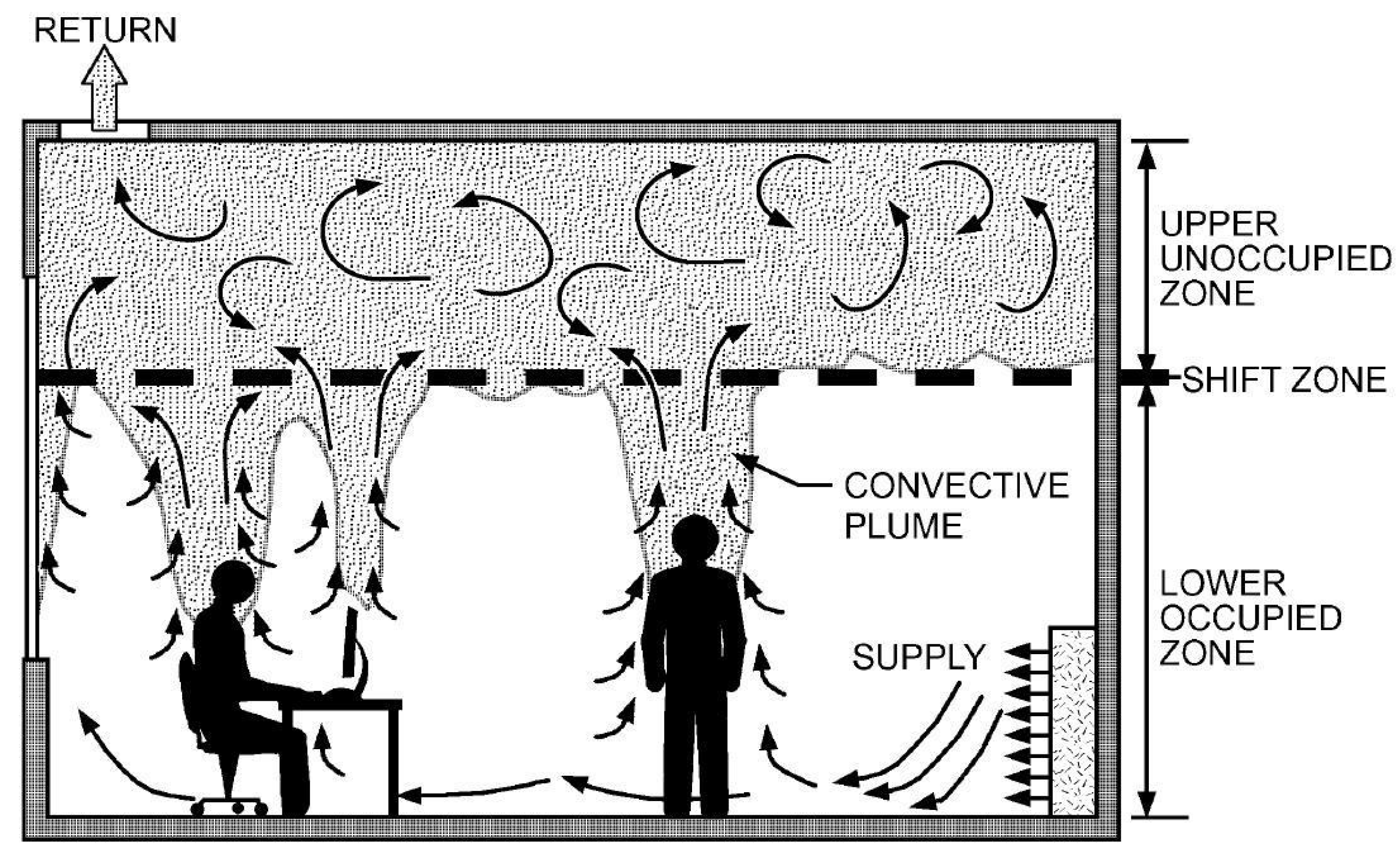
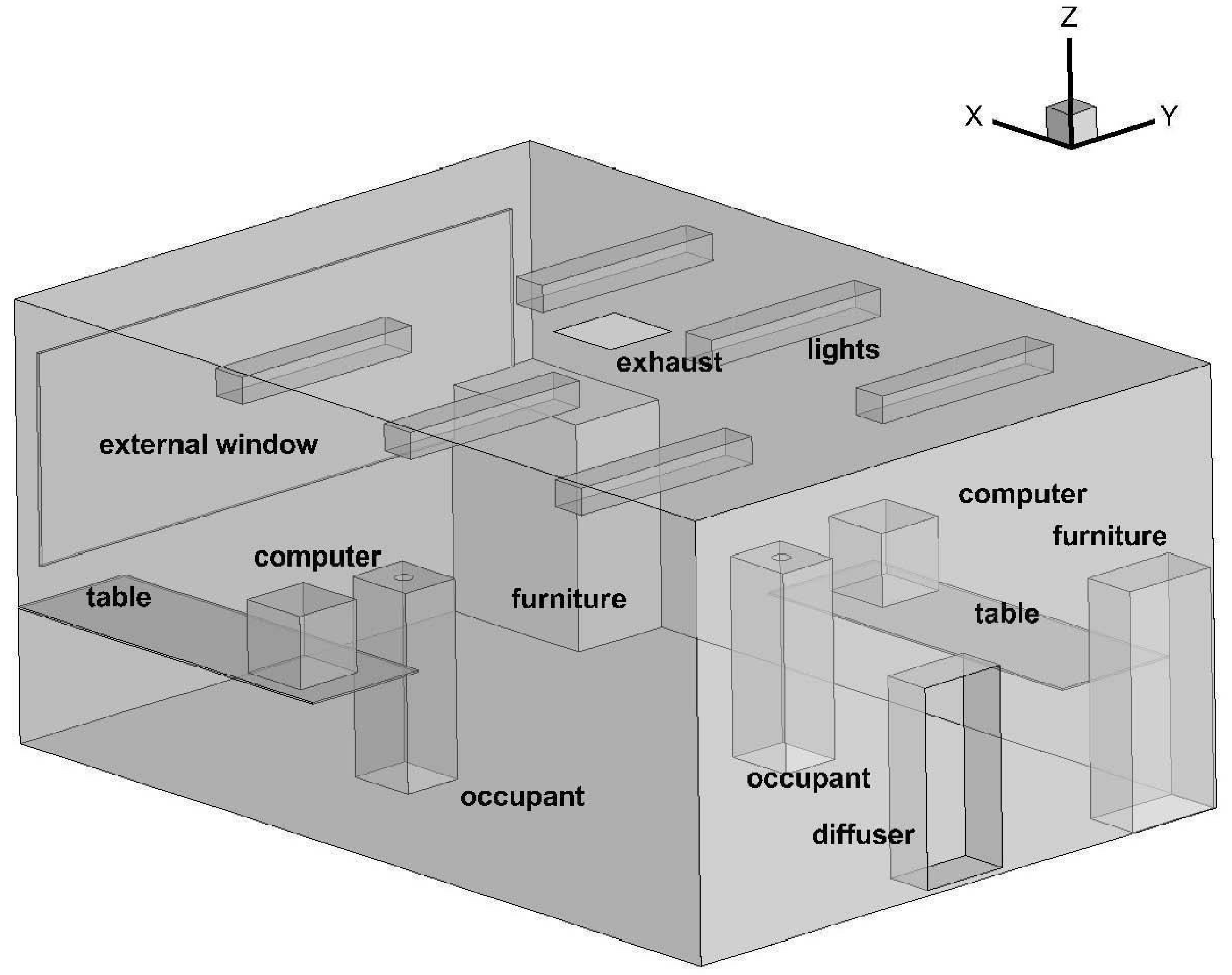
3. Application: An Office Room Equipped with Thermal Displacement Ventilation System

An optimization case is designed using the proposed framework. In this case study, an office room equipped with a TDVS is constructed. As is known, for displacement ventilation systems, a vertical temperature gradient should exist because it indicates a stratified airflow pattern and vertical stratification of contaminants. Consequently, two distinct zones are formed for TDVS (Figure 2): a lower occupied zone with little or no recirculation flow, and an upper zone with recirculation flow [24]. The simplified temperature profile in the space is already well understood by many previous studies. However, to deal with conflicting design criteria, such as thermal comfort, IAQ, and energy savings, the designers still lack necessary analysis to understand the behavior of such multi-objective optimization issues.

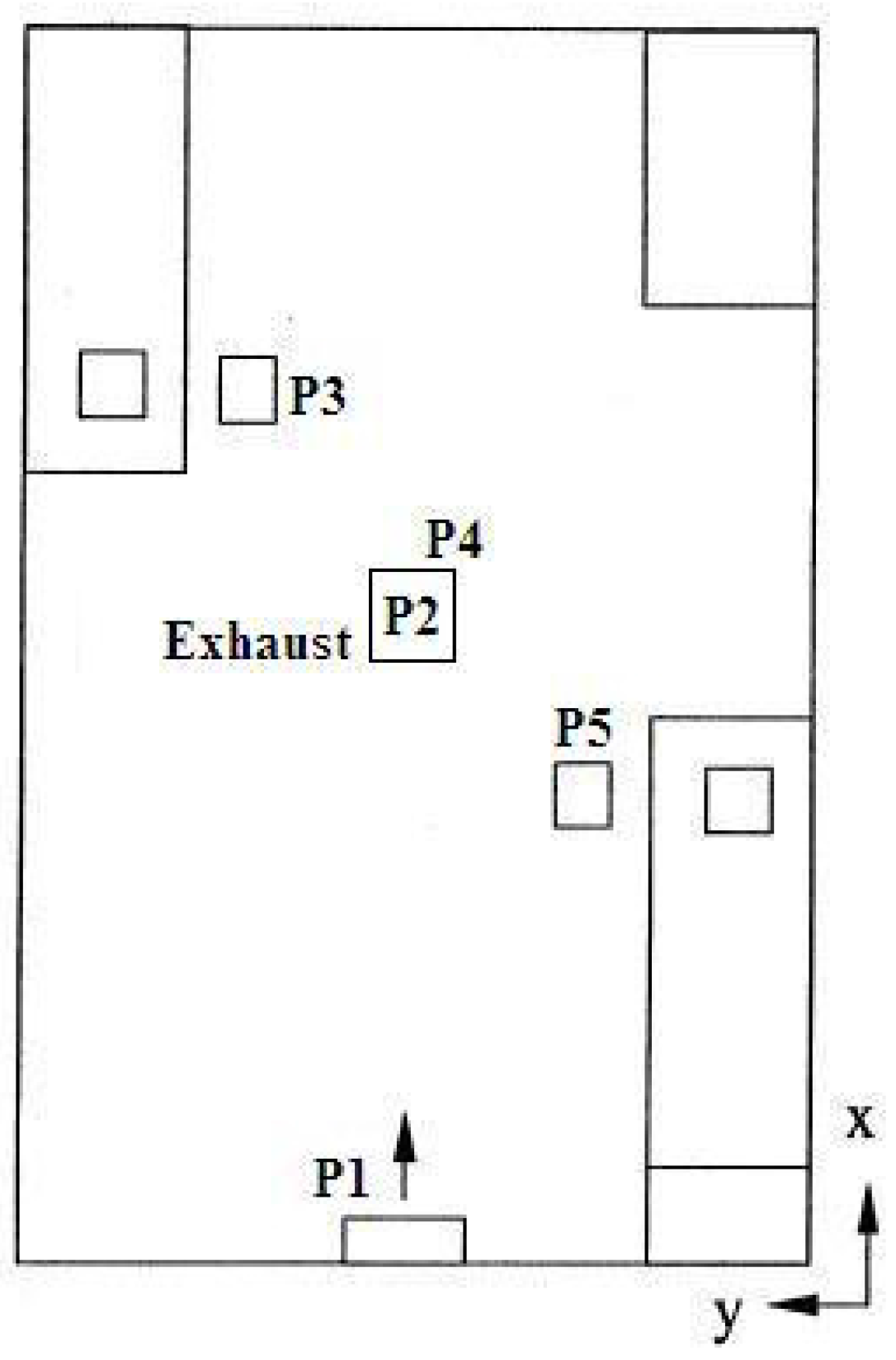
3.1. Model Description

The indoor thermal environment of buildings is a typical kind of complex PDE system. It is because temperature fields are thermally coupled with the airflow distribution that is generally governed by the incompressible Navier–Stokes equations. The continuity, momentum, and energy equations in non-dimensional form are shown as follows:

$$\begin{array}{c}\hfill \left\{\begin{array}{cc}& \nabla \times \mathit{V}=0\hfill \\ & \frac{\partial \mathit{V}}{\partial t}=-(\mathit{V}\times \nabla )\mathit{V}+\frac{1}{Re}{\nabla }^2\mathit{V}-\nabla p+\frac{Gr}{R{e}^2}\theta \delta \hfill \\ & \frac{\partial \theta }{\partial t}=-\mathit{V}\times \nabla \theta +\frac{1}{RePr}{\nabla }^2\theta \hfill \end{array}\right.\end{array}$$

(2)

in the domain Ω $\times [0,\theta ]$, where Ω represents a spatial domain, δ is a unit vector in the direction of gravitational acceleration, the Prandtl number $Pr=\mu c_p/\kappa$, Grashof number $Gr=\beta {\ell }^{3}g\Delta \theta /{\nu }^2$, and Reynolds number $Re=V_{max}\ell /\nu$.

A two-person office room of $5.16$ m length, $3.65$ m width, and $2.43$ m height (Figure 3) is modeled, which was investigated experimentally by Yuan et al. [25]. The room is equipped with two tables, two heated computers, two file cabinets, and six overhead lights. A $3.65$ m × $1.04$ m window is mounted on the left wall. A perforated displacement diffuser (0.5 m × 1.1 m) is placed at the middle of the right side wall near the floor. The exhaust (0.43 m × 0.43 m) is at the center of the ceiling. The two sitting occupants in the test room are simulated by two boxes of 0.4 m × 0.35 m × 1.1 m. Two point sources of CO${}_2$ are introduced at the top of the two boxes to simulate contaminants from the occupants, with an initial velocity of 0.045 m/s in the horizontal direction. The other details of office configuration can be found in

Table 1. The main parameters of the office layout.

Entry	Length	Width	Height	Heat
	$\mathbf{\Delta }\mathit{x}$ (m)	$\mathbf{\Delta }\mathit{y}$ (m)	$\mathbf{\Delta }\mathit{z}$ (m)	Q (W)
Room	5.16	3.65	2.43	-
Diffuser	0.28	0.53	1.11	-
Exhaust	0.43	0.43	0.0	-
Occupant	0.4	0.35	1.1	75
PC	0.4	0.4	0.4	108.5
Table	2.23	0.75	0.01	0.0
Window	0.02	3.35	1.16	0.0
Furniture	0.95	0.58	1.24	0.0
Light	0.2	1.2	0.15	34

and [25].

3.2. Assessment Indices

In this study, we regulate supply air temperature and flow speed of TDVS, aiming to improve the thermal comfort and IAQ in the occupied zones, considering the energy consumption of TDVS. Because CFD simulation offers more detailed information of indoor dynamic behavior than other methods [24], we can extract various of environmental parameters precisely at any location within the computing domain for the optimization issue. Here, three assessment indices are set as follows.

3.2.1. Thermal Discomfort Index

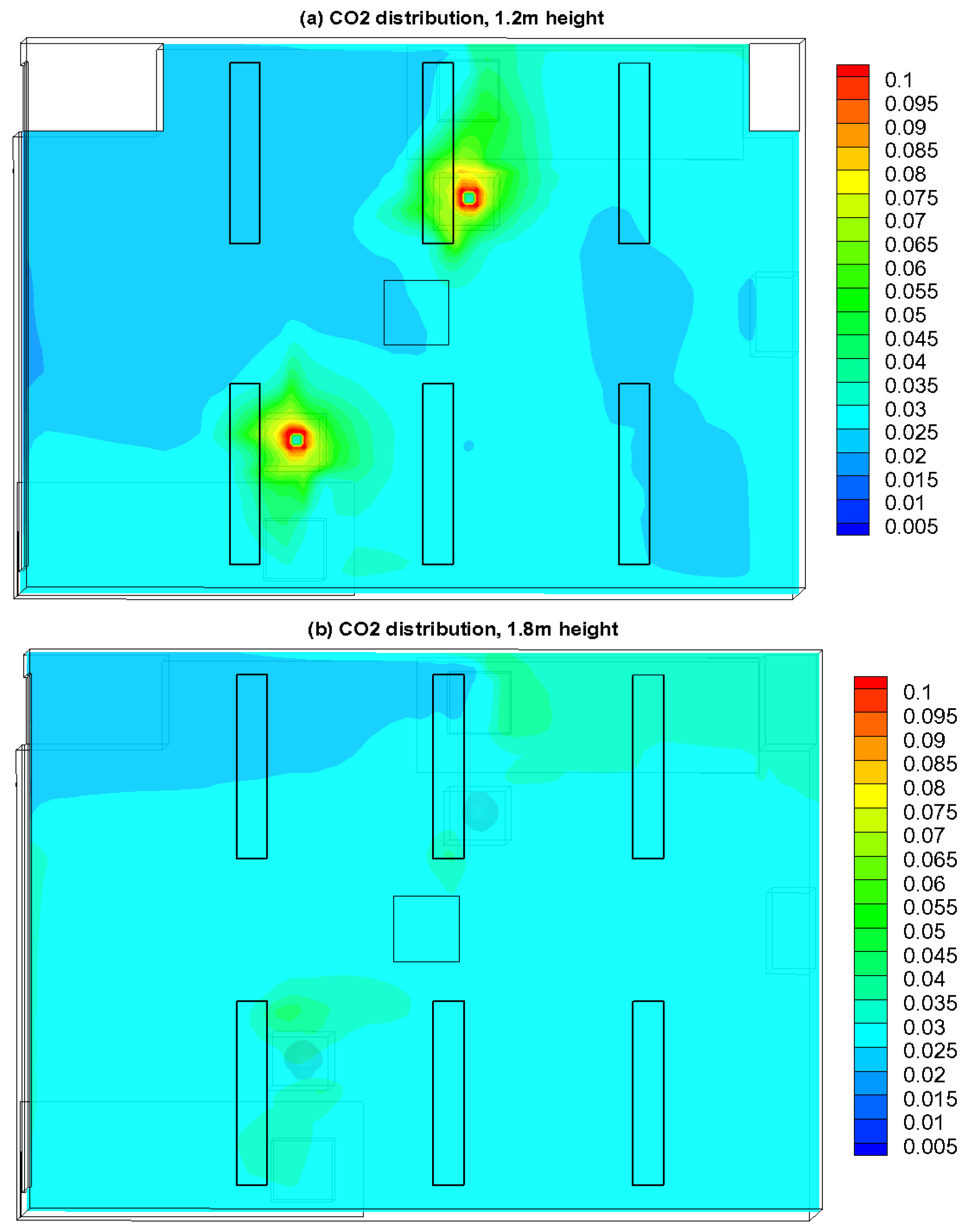
The predicted mean vote-predicted percent dissatisfied (PMV-PPD) model [26] is the most frequently used and best understood model for quantitative thermal comfort analysis. PMV reflects the mean thermal sensation vote on a standard scale for a large group of occupants. In order to predict the thermal comfort conditions, PMV combines six thermal variables related to the indoor air conditions and human behaviors, including air temperature, air humidity, air velocity, mean radiant temperature, clothing insulation level, and human activity. PPD reflects the percentage of thermally dissatisfied persons among a large group of occupants. It can be evaluated by the formula below:

$$PPD=100-95\times \exp (-0.03352\times PM{V}^4-0.2179\times PM{V}^2)$$

(3)

According to ISO7730 and ASHRAE 55-2004 [27], the proper value of the index PMV is between $-0.5$ and $+0.5$ ($PPD\le 10\%$). In this study, the index PPD is preferred to PMV because it provides an objective function to minimize, which is fundamental for running the optimization algorithm.

3.2.2. CO${}_2$-Based Ventilation Effectiveness

Indoor air quality is an important concern in building systems. Supplying fresh outdoor air and removing air pollutants is necessary for the maintenance of acceptable IAQ levels. However, ventilation rates inside buildings must be seriously reduced in order to optimize the cooling or thermal load in an improved manner and save the energy load. To access the effect of airborne contaminants removal, there are several frequently used IAQ indexes, such as Age of Air [28], Contaminant Removal Efficiency ($E_c$), Ventilation Effectiveness ($E_v$) [29], and Re-inhaled Exposure Index ($E_{RI}$) [30]. In this study, CO${}_2$ is injected into the space as airborne contaminants [31], and the index ventilation effectiveness (${\epsilon }_v$) is used for IAQ assessment, which is formulated as:

$${\epsilon }_v=\frac{C_{return}-C_{supply}}{C_{br}-C_{supply}}$$

(4)

where $C_{return}$ is the CO${}_2$ concentration in the return air (mass fraction), $C_{supply}$ is the CO${}_2$ concentration in the supply air, and $C_{br}$ is the CO${}_2$ concentration at breathing level near the occupant.

3.2.3. Energy Consumption

Based on the survey of previous experimental and numerical work on quantifying the energy efficiency of ventilation systems [7,32], we divide the energy usage of the ventilation system into two parts: fan power input and cooling energy consumption.

Basically, fan power input (W) can be determined using the following expression:

$$E_{fan}=\frac{\Delta P\times {\stackrel{·}{V}}_{air}}{1000{\eta }_{fan}}$$

(5)

where $\Delta P$ is the pressure rise through the supply fan (Pa), ${\stackrel{·}{V}}_{air}$ is the overall volumetric flow rate of supply air (L/s), and ${\eta }_{fan}$ is the fan efficiency. For simplicity, the pressure rise and fan efficiency are assumed to be 562.5 Pa and 0.75, respectively.

The cooling energy requirement is subdivided into two portions: the sensible heat load produced within the conditioned space and the cooling load due to the fresh air treatment, which is shown below:

$$E_{cooling}=E_{space}+E_{vent}={\stackrel{·}{m}}_{air}{c}_p(T_{return}-T_{supply})+{\stackrel{·}{m}}_{fresh}(h_{out}-h_{return})$$

(6)

where ${\stackrel{·}{m}}_{air}$ is the total mass flow rate of supply air (kg/s), $c_p$ is the specific heat of air (J/kg·k), $T_{return}$ and $T_{supply}$ are the temperature of return air and supply air (k), respectively, and ${\stackrel{·}{m}}_{fresh}$ is the mass flow rate of outdoor fresh air (kg/s). $h_{out}$ and $h_{return}$ are the specific enthalpy of the outdoor air and return air (J/kg), which can be formulated with relative humidity and temperature as:

$$h=1.01\times t+0.001\times d(2500+1.84\times t)$$

(7)

where d is relative humidity of air.

Some of the parameters mentioned above are directly obtained by CFD simulations, including ${\stackrel{·}{V}}_{air}$, ${\stackrel{·}{m}}_{air}$, $T_{return}$, and $T_{supply}$. The others are set according to literature and experience. ${\stackrel{·}{m}}_{fresh}$ is assumed to be 30% of the total supply air, and the relative humidity is assumed to be maintained at a constant level (50% indoor [32] and 70% outdoor [33]). Air density and specific heat are set to constant values, at 1.225 kg/m${}^3$ and 1006.43 J/kg${}^{\circ }\mathrm{C}$, respectively.

It should be noted that the focus of this study is on the applicability of the proposed optimization strategy, and the energy assessment is simplified in several respects:

*

The energy consumption of water pump and reheat system are neglected;

*

The heat exchange efficiency of each component of the HVAC system is assumed as 1;

*

The pipeline is assumed to be thermally insulated, and air flow inside it has no energy loss.

3.3. Multi-Objective Functions for Optimization

Indoor climate regulation is a multivariate problem having no unique solution. In this study, the goals of the optimization strategy include:

(1)

High thermal comfort level: guarantee a high comfort level in the occupied zone of the office room.

(2)

Acceptable IAQ level: supply fresh outdoor air and remove air pollutants to maintain an acceptable IAQ level.

(3)

Energy savings: save energy cost without sacrificing thermal comfort and IAQ levels.

Accordingly, the optimization problem can be mathematically expressed as:

$$\min \{PP{D}^{max},IA{Q}^{avg},E_{fan+cooling}\}$$

where $PP{D}^{max}$ is the maximum value of PPD in the occupied zones. We believe that $PP{D}^{max}$ is preferred to the average value as objective function, because it allows a more rigorous control of thermal comfort. To provide an objective function of IAQ level to minimize, $IA{Q}^{avg}$ is set as $1/{\epsilon }_v^{avg}$ to represent the average value of ventilation effectiveness at breathing level near the two occupants; $E_{fan+cooling}$ is the sum of $E_{fan}$ and $E_{cooling}$ of the ventilation system.

4. Results and Analysis

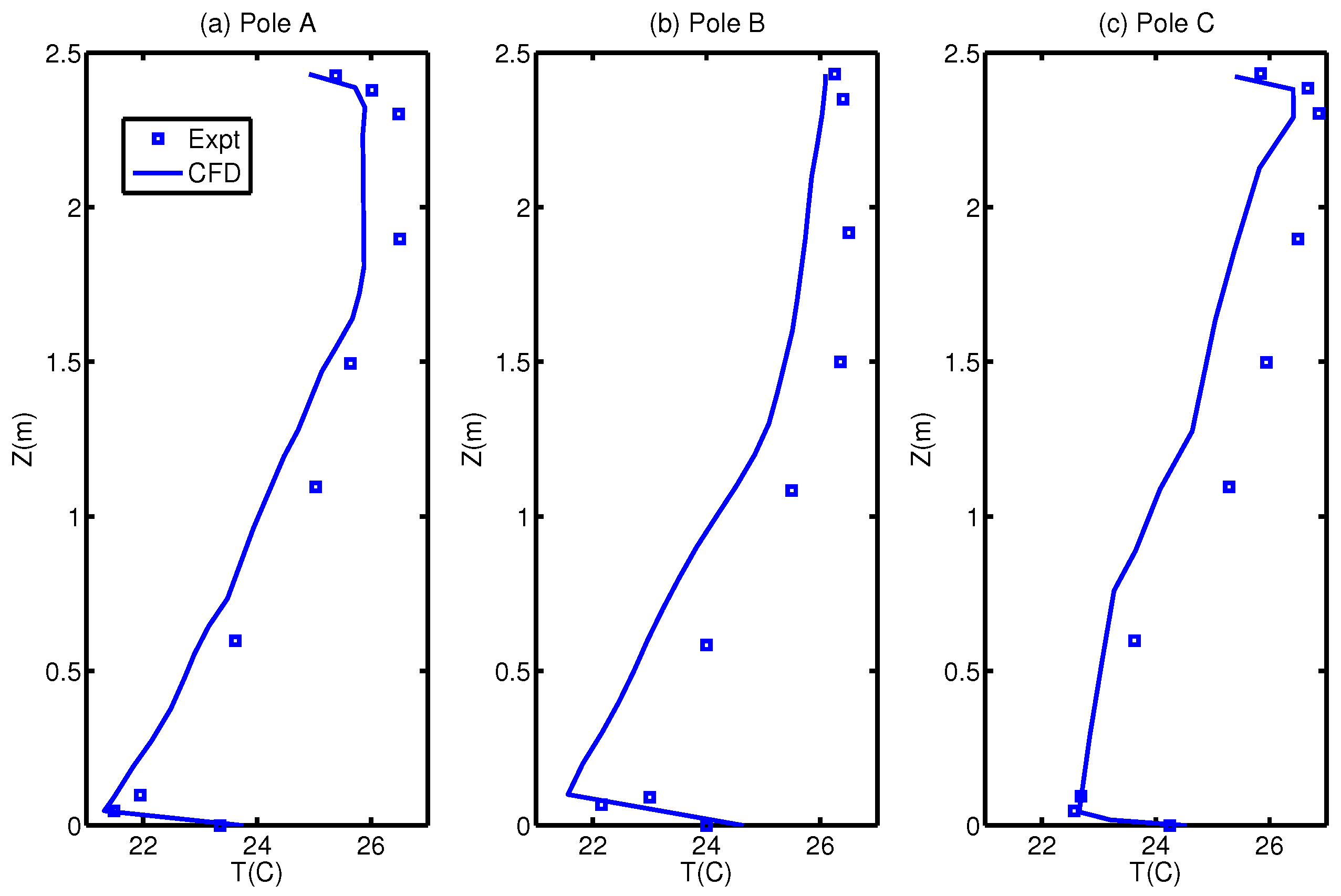
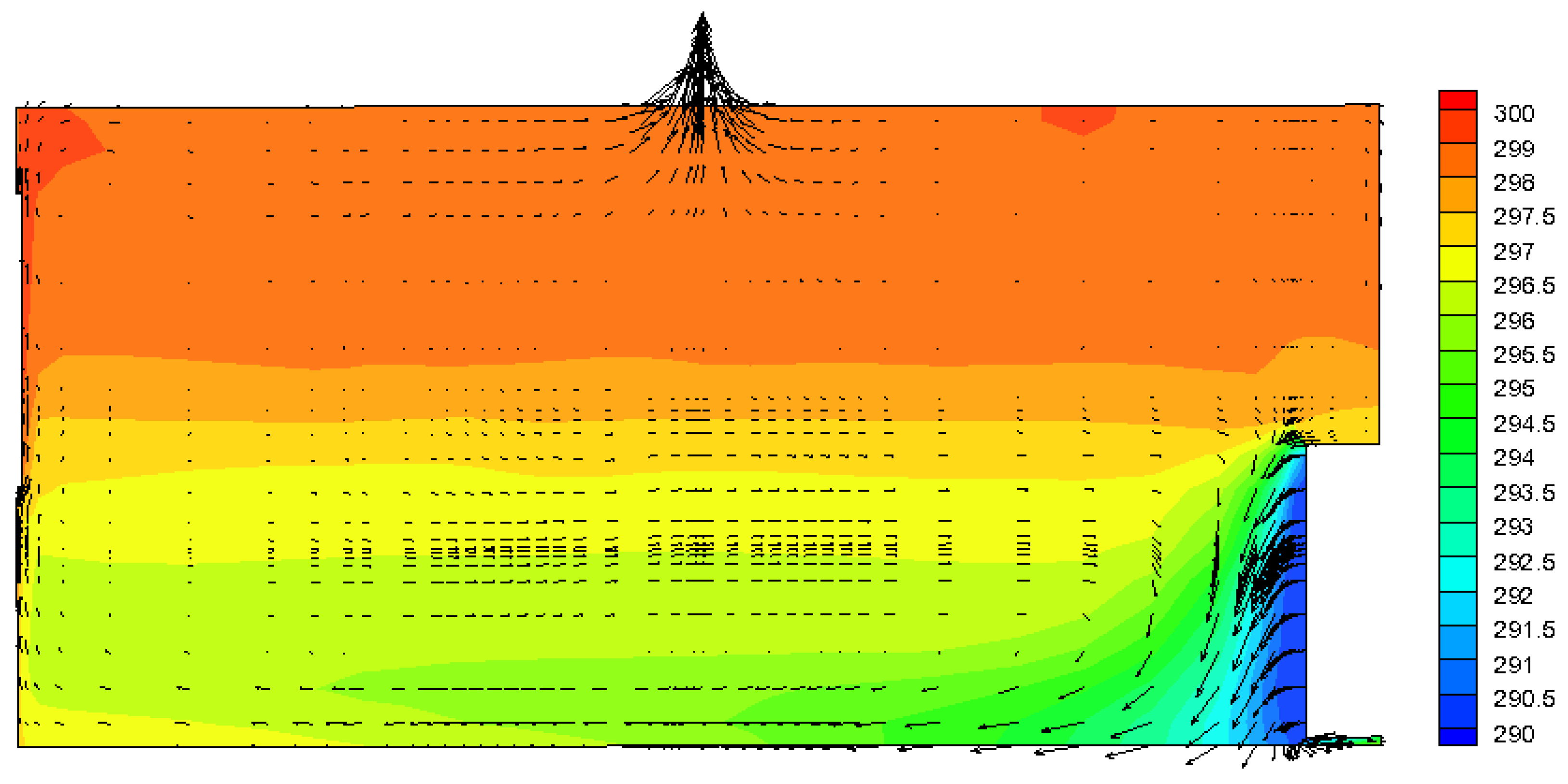
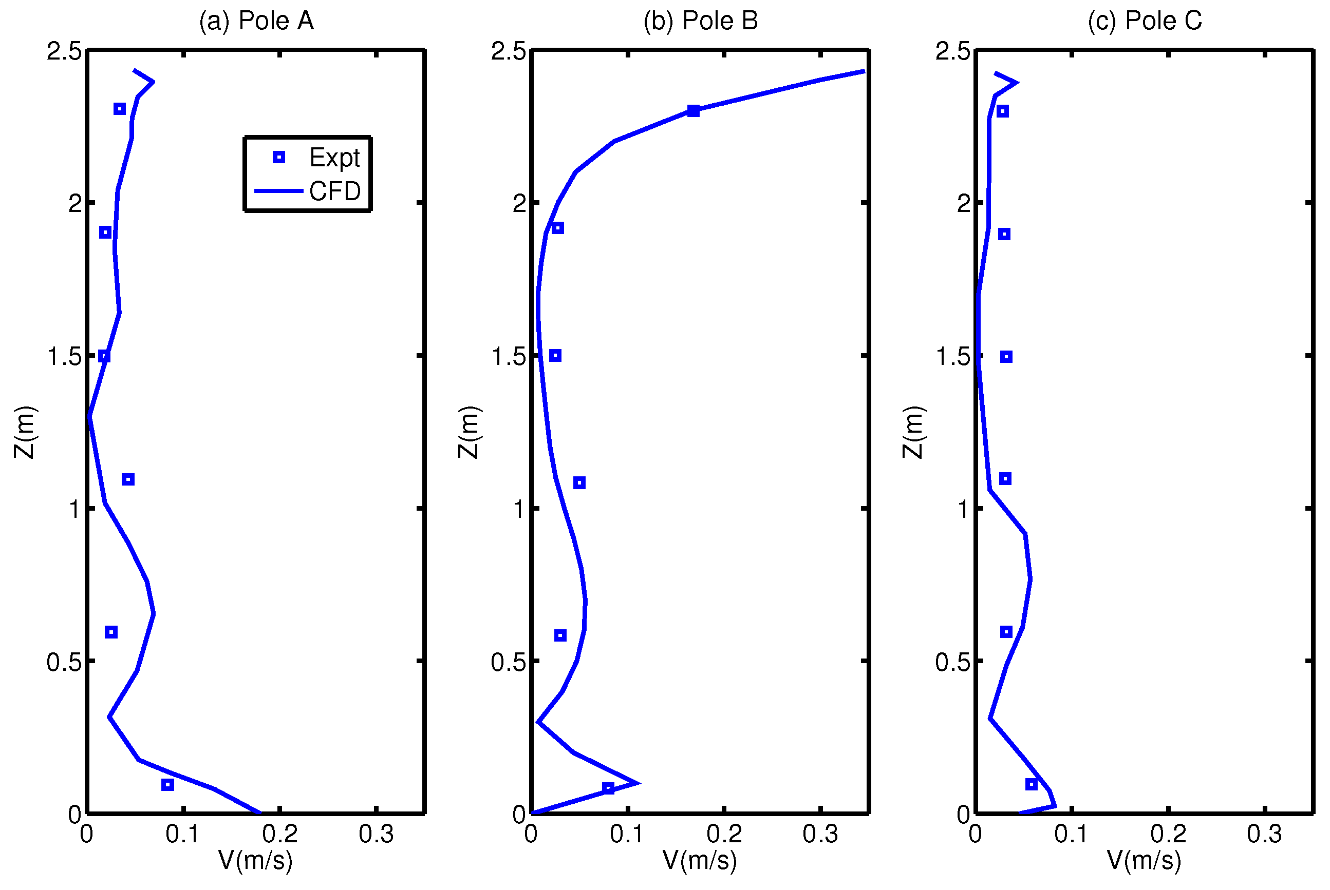
4.1. Validation of Computational Fluid Dynamic Simulation

The main parameters of the simulation are set as follows: RNG $\kappa -\epsilon$ model for turbulence, standard wall functions for near-wall treatment, buoyancy effects under consideration using Boussinesq’s approximation and no viscous heating. The inner surface temperature is set as 24.65 ${}^{\circ }\mathrm{C}$, and CO${}_2$ emission rate is 0.87 L/min. In order to validate the CFD model, the supply air temperature and velocity are set at 17 ${}^{\circ }\mathrm{C}$ and 0.09 m/s as [25]. It is known that the more grids used, the more accurate the results will be. But a fine grid will cost more optimization time and capacity. In this study, the corresponding prediction solved the 3D mass, momentum, energy, and concentration equations on the computing domain containing non-uniform 172,282 nodes. Airpak software with Fluent engine is used to build the validated office model.

Figure 4 shows the simulation results of the CFD model. The steady temperature contour and airflow pattern are recorded at mid-vertical plane through the diffuser. From the figure, the fully-stratified air distribution is clearly observed. To compare the simulation results with measured data, three poles are set in the mid-vertical plane: Pole A (x: 1.75 m, y: 1.825 m), Pole B (x: 2.65 m, y: 1.825 m), and Pole C (x: 3.55 m, y: 1.825 m). The simulated temperature and velocity at the three poles are extracted and compared with the measurements reported in [25] (Figure 5 and Figure 6). The agreement between the computed results and measured data demonstrate the availability of the CFD model.

4.2. Construction of the Optimization Case

Based on the framework described in Section 2.2, the optimization case using the proposed data interactive mechanism is set up. The temperature and airspeed of the diffuser are set as control variables with the variation ranges: 290–298 K and 0.05–1.5 m/s. In order to record environmental parameters during the optimization procedure, five virtual points (P1–P5, see Figure 7) are set in the computing domain. P1 and P2 are set at the diffuser and exhaust of the room, respectively. P3, P4, and P5 are set at the occupied zone that is near the top of simulated occupants. At the end of each iteration, steady temperature, air speed, and CO${}_2$ concentration at the recording points are automatically saved to $Sim\_outputfiles$ (Airpak*.out), which will be read by interactive module for objectives evaluation. We realized the multi-objective-based genetic algorithm (NSGA-II) on the basis of Kalyanmoy Deb’s report [21]. Three objective functions are defined according to Section 3.2’s discussion, which are evaluated by parameters passing using data interactive module every iteration.

As is known, a full CFD calculation is time-consuming. On the basis of ensuring convergence, CFD-related parameters are set to speed up the whole optimization procedure, such as setting an appropriate initial value, applying a first-order discretization scheme, setting the main equations’ convergence criteria to ${10}^{-3}$, and shortening the number of iterations. Further, the population size and maximum number of generations are both chosen as 25.

Table 2. Main parameters of the optimization case. NSGA-II: non-dominated-and-crowding Sorting Genetic Algorithm II.

Category	Parameter	Design Range
CFD	Inlet air speed	0.05–1.5 m/s
	Inlet temperature	290–298 K
	velocity of CO${}_2$ emission	0.045 m/s
	Number of iterations	250
NSGA-II	Number of generations	25
	Population size	25
	Crossover probability	0.8
	Number of elites produced	2

specifies the main parameters of this case study. With the above parameter settings, the whole optimization procedure requires about 72 h to obtain the Pareto front. The computer used to run the simulation is an Intel Core E3 (4 cores, 3.2 GHz) with 8 GB of RAM. It is noted that the optimization time is sensitive to the parameter settings. If we increase some parameter values, such as number of iterations, number of generations, or population size, the optimization procedure will take longer.

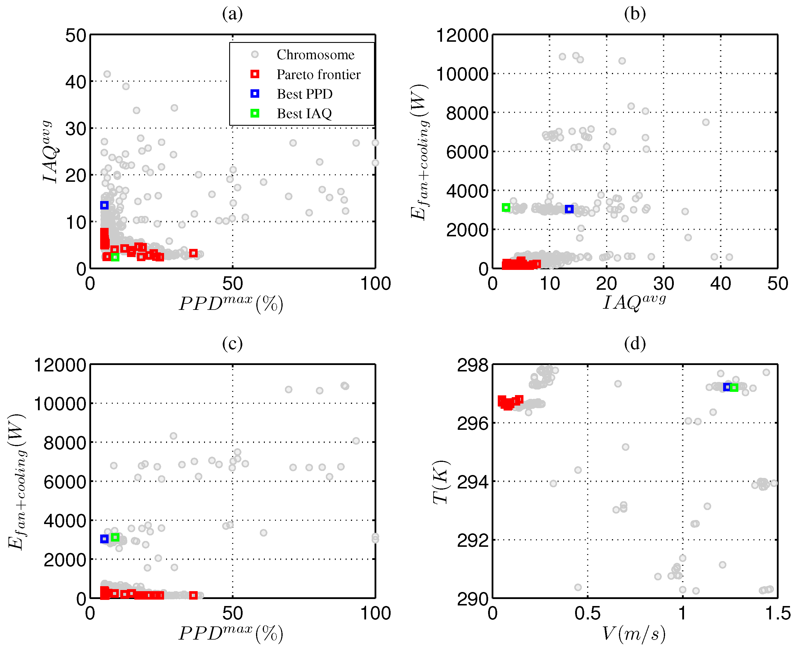
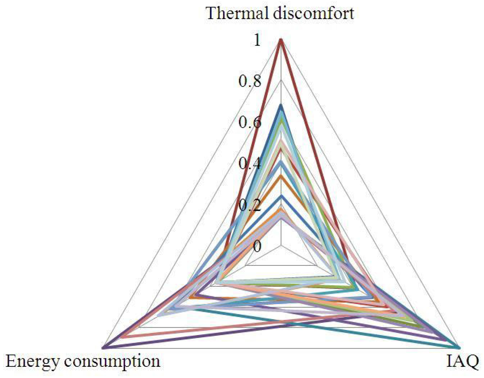
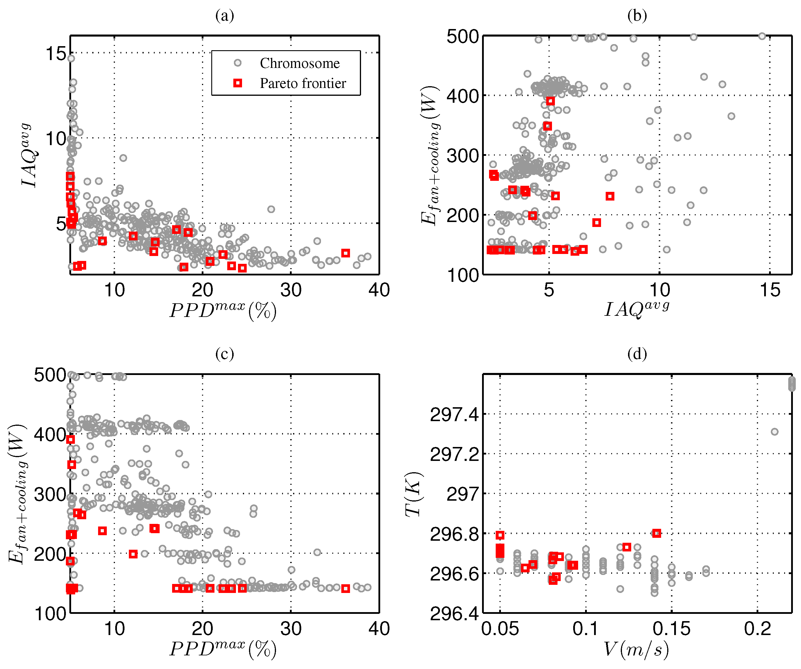
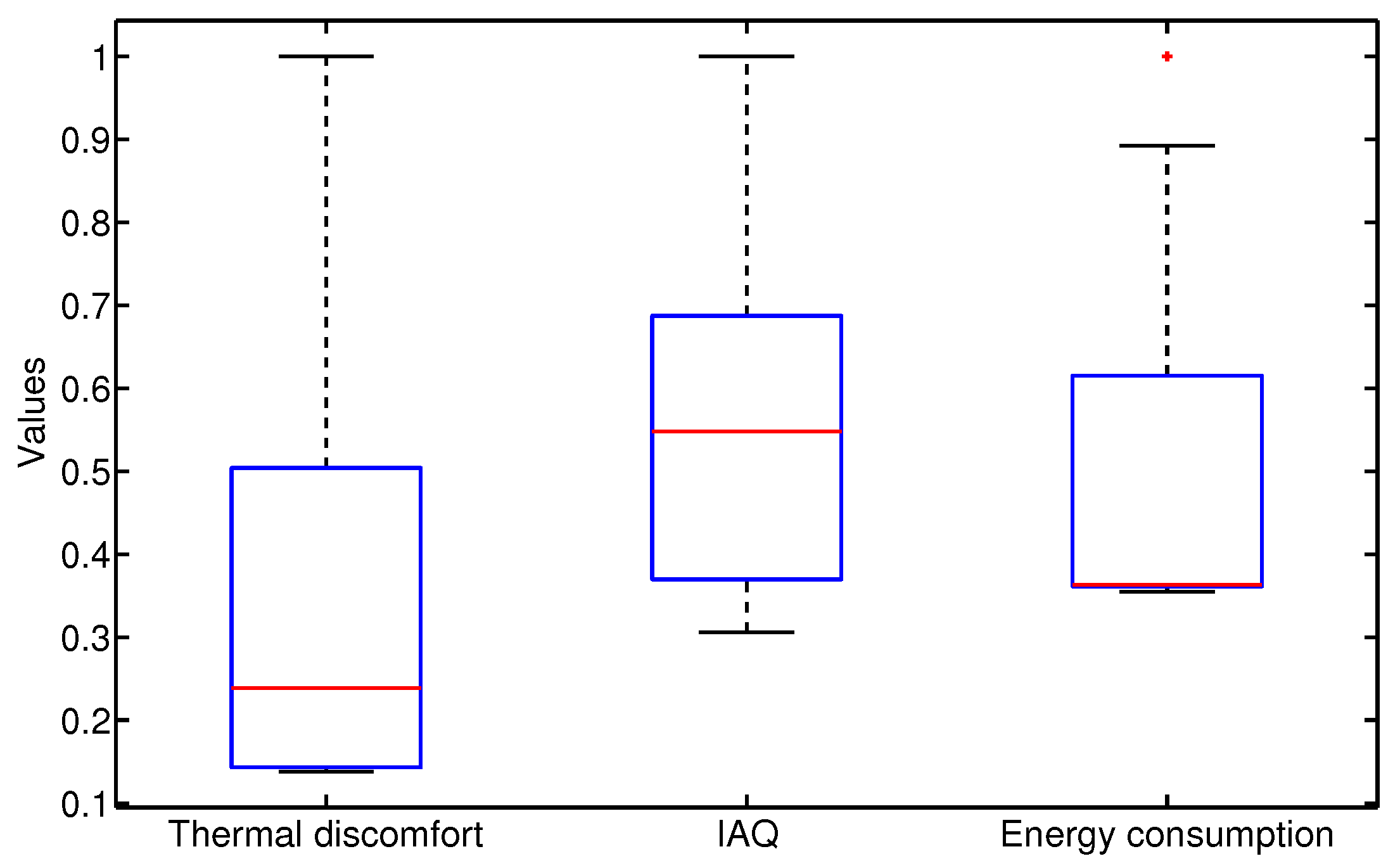
4.3. Analysis of the Pareto Frontiers

The results of the multi-objective optimization are represented graphically, since the visualization of the Pareto front makes the interpretation of the results direct. We compare every two objective functions at a time by projecting the 3D-Pareto front on bi-dimensional (2D) graphs (Figure 8). Each of the 2D-graphs provides information about a specific behavior that allows various aspects of the optimization run to be discussed; i.e., (i) thermal comfort performance; (ii) IAQ performance; (iii) energy consumption performance.

From a total of 648 chromosomes, the 25 pairs of control variables of the last generation identified by the NSGA-II algorithm belong to the Pareto front, and are considered the optimal control variables according to the presented 3D-optimization case. In Figure 8a–c, it is found that each of those variables performs quite differently with respect to the individual objective functions. Among the best solutions, the variations of the index of IAQ level ($IA{Q}^{avg}$) and energy consumption ($E_{fan+cooling}$) are quite limited, while the thermal discomfort index ($PP{D}^{max}$) has a large spread.

From Figure 8d, it is shown that 25 pairs of control variables are clustered in two groups. In the two 2D projections of objective space (IAQ–Energy and PPD–Energy graphs), the cluster effect is also easily identified. By quantitative analysis of the two clusters, the group containing most solutions (23/25) has energy consumption lower than 500 W. The other group containing two solutions (marked with green and blue colors in Figure 8) has much higher energy consumption beyond $2000\mathrm{W}$. However, the green one represents the best solution that acquires the optimal IAQ level (minimum of $IA{Q}^{avg}$: 2.40) and the blue one reaches the optimal thermal comfort (minimum of PPD: 5.00). This means that when thermal and IAQ optimization are coupled with energy consumption optimization, the optimal option is not simple to obtain.

If we limit the energy consumption below 500 W and redraw the figure (Figure 9), 23 solutions remain in the Pareto front with more clear distribution shapes. Theoretically, the set of all variables on the Pareto front are solutions of the multi-objective optimization problem. The outcomes of this specific limitation show that most optimal control variables can reach values of $E_{fan+cooling}$ lower than 400 W, $PP{D}^{max}$ less than 25% (12 solutions less than 10%) and $IA{Q}^{avg}$ less than 10, simultaneously. At the same time, from Figure 9d we can find that most of the optimal air speeds of the diffuser are between 0.05 m/s and 0.1 m/s , and the optimal temperate is between 296.5 K and 297 K. The control variables that fell into above ranges are consistent with the American Society of Heating Refrigerating and Air conditioning Engineer (ASHRAE) standard’s recommendation [24,27]. It is noted that, in practice, both flow rate and supply temperature are connected to meeting the load and are constrained by temperature gradient condition and stratification height condition, which are ignored in this optimization study.

In order to derive the emphasis of different solutions, each building index belonging to the 3D Pareto front is represented on a radar diagram (Figure 10). To ensure that no special axis is dominant over the others, all types of indexes are normalized to the interval (0, 1) by a simple linear scaling function: $X_i=x_i/x_{max},i=1,2,...,23$. The distributions of the building indexes are also represented in boxplots (Figure 11). As discussed above, the variations of the index of energy consumption ($E_{fan+cooling}$) are quite limited. Almost half are clustered at the bottom of the box (near 140 W). Such results show that by satisfying the used PMV and IAQ indexes, the HVAC system’s energy conservation still has the potential if the occupied zone’s environmental parameters can be precisely fed back by sensors.

Finally, one of the best 23 solutions is chosen from the 3D Pareto front for full simulation. The steady CFD simulation is carried out (inlet air speed: 0.07 m/s, inlet temperature: 296.68 K). For this solution, the $PP{D}^{max}$ is reached at about 5.08%, IAQ level ($IA{Q}^{avg}$) is 2.4, and $E_{fan+cooling}$ is calculated as about 140 W. To roughly describe the ventilation effectiveness, the distributions of CO${}_2$ fraction at sitting and standing heights are shown in Figure 12. It should be noted that the study case is a simulation-based model. The optimization results are valid on the basis of some assumptions and simplicities, such as the simplified energy assessment, the temperature boundary conditions, etc.

5. Conclusions

This study presents a CFD-coupled optimization framework to explore the Pareto front of thermal comfort, IAQ, and energy consumption of the indoor environment of buildings. A numerical optimization case is constructed according to the established framework. Results show that the optimized control variables are consistent with the ASHRAE standard’s recommendation. The analysis of the Pareto frontiers also finds the potential of the HVAC system’s energy conservation. It could be generalized that, for designing HVAC operations optimized with respect to multiple nonlinear objectives, advanced optimization techniques such as this study’s framework are required to effectively support designers in selecting and analyzing suitable solutions.

The next research step will be as follows: 1. Compare different multi-objective optimization algorithms with one CFD model. 2. Optimization of air supply location and size in an enclosed environment using the proposed CFD-coupled optimization method.

References

1. Perez-Lombard, L.; Ortiz, J.; Pout, C. A review on buildings energy consumption information. Energy Build. 2008, 40, 394–398. [Google Scholar] [CrossRef]
2. Tsinghua University Building Efficiency Research Center. 2015 Annual Report on China Building Energy Efficiency; China Building Industry Press: Beijing, China, 2015. (In Chinese) [Google Scholar]
3. IFMA Survey Ranks Top 10 Office Complaints; Technical Report; International Facility Management Association (IFMA): Houston, TX, USA, 2012.
4. Novoselac, A.; Srebric, J. A critical review on the performance and design of combined cooled ceiling and displacement ventilation systems. Energy Build. 2002, 34, 497–509. [Google Scholar] [CrossRef]
5. Lee, J.H. Optimization of indoor climate conditioning with passive and active methods using GA and CFD. Build. Environ. 2007, 42, 3333–3340. [Google Scholar] [CrossRef]
6. Heidarinejad, G.; Fathollahzadeh, M.H.; Pasdarshahri, H. Effects of return air vent height on energy consumption, thermal comfort conditions and IAQ in an under floor air distribution system. Energy Build. 2015, 97, 155–161. [Google Scholar] [CrossRef]
7. Zhou, L.; Haghighat, F. Optimization of ventilation system design and operation in office environment, Part I: Methodology. Build. Environ. 2009, 44, 651–656. [Google Scholar] [CrossRef]
8. Zhou, L.; Haghighat, F. Optimization of ventilation systems in office environment, Part II: Results and discussions. Build. Environ. 2009, 44, 657–665. [Google Scholar] [CrossRef]
9. Asadi, E.; da Silva, M.G.; Antunes, C.H.; Dias, L.; Glicksman, L. Multi-objective optimization for building retrofit: A model using genetic algorithm and artificial neural network and an application. Energy Build. 2014, 81, 444–456. [Google Scholar] [CrossRef]
10. Li, K.; Xue, W.; Xu, C.; Su, H. Optimization of ventilation system operation in office environment using POD model reduction and genetic algorithm. Energy Build. 2013, 67, 34–43. [Google Scholar] [CrossRef]
11. Yu, W.; Li, B.; Jia, H.; Zhang, M.; Wang, D. Application of multi-objective genetic algorithm to optimize energy efficiency and thermal comfort in building design. Energy Build. 2015, 88, 135–143. [Google Scholar] [CrossRef]
12. Kim, T.; Song, D.; Kato, S.; Murakami, S. Two-step optimal design method using genetic algorithms and CFD-coupled simulation for indoor thermal environments. Appl. Therm. Eng. 2007, 27, 3–11. [Google Scholar] [CrossRef]
13. Palonen, M.; Hasan, A.; Siren, K. A genetic algorithm for optimization of building envelope and HVAC system parameters. In Proceedings of the 11-th IBPSA Conference, Glasgow, UK, 27–30 July 2009; pp. 159–166.
14. Coffey, B.; Haghighat, F.; Morofsky, E.; Kutrowski, E. A software framework for model predictive control with GenOpt. Energy Build. 2010, 42, 1084–1092. [Google Scholar] [CrossRef]
15. Asadi, E.; Silva, M.; Antunes, C.; Dias, L. A multi-objective optimization model for building retrofit strategies using TRNSYS simulations, GenOpt and MATLAB. Build. Environ. 2012, 56, 370–378. [Google Scholar] [CrossRef]
16. Futrell, B.J.; Ozelkan, E.C.; Brentrup, D. Bi-objective optimization of building enclosure design for thermal and lighting performance. Build. Environ. 2015, 92, 591–602. [Google Scholar] [CrossRef]
17. Liu, W.; Chen, Q. Optimal air distribution design in enclosed spaces using an adjoint method. Inverse Probl. Sci. Eng. 2015, 23, 760–779. [Google Scholar] [CrossRef]
18. Liu, W.; Jin, M.; Chen, C.; Chen, Q. Optimization of air supply location, size, and parameters in enclosed environments using a computational fluid dynamics-based adjoint method. J. Build. Perform. Simul. 2016, 9, 149–161. [Google Scholar] [CrossRef]
19. Jasak, H.; Jemcov, A.; Tukovic, Z. A C++ library for complex physics simulations. In Proceedings of the International Workshop on Coupled Methods in Numerical Dynamics, Dubrovnik, Croatia, 19–21 September 2007.
20. Goldberg, D.E. Genetic algorithm approach: Why, how, and what next? Adapt. Learn. Syst. Theory Appl. 1986, 1985, 247–253. [Google Scholar]
21. Deb, K.; Pratap, A.; Agarwal, S.; Meyarivan, T. A fast and elitist multiobjective genetic algorithm: NSGA-II. IEEE Trans. Evol. Comput. 2002, 6, 182–197. [Google Scholar] [CrossRef]
22. McKinstray, R.; Lim, J.B.; Tanyimboh, T.T.; Phan, D.T.; Sha, W.; Brownlee, A.E. Topographical optimisation of single-storey non-domestic steel framed buildings using photovoltaic panels for net-zero carbon impact. Build. Environ. 2015, 86, 120–131. [Google Scholar] [CrossRef]
23. Murray, S.N.; Walsh, B.P.; Kelliher, D.; O’Sullivan, D. Multi-variable optimization of thermal energy efficiency retrofitting of buildings using static modelling and genetic algorithms—A case study. Build. Environ. 2014, 75, 98–107. [Google Scholar] [CrossRef]
24. American Society of Heating, Refrigerating and Air-Conditioning Engineers (ASHRAE). ASHRAE Handbook 2007: Room Air Distribution; ASHRAE: Atlanta, CA, USA, 2007. [Google Scholar]
25. Yuan, X.; Chen, Q.; Glicksman, L.; Hu, Y.; Yang, X. Measurements and computations of room airflow with displacement ventilation. ASHRAE Trans. 1999, 105, 340–352. [Google Scholar]
26. Fanger, P. Thermal Comfort: Analysis and Applications in Environmental Engineering; McGraw-Hill: New York, NY, USA, 1972. [Google Scholar]
27. American Society of Heating, Refrigerating and Air-Conditioning Engineers (ASHRAE). ANSI/ASHRAE Standard 55-2004: Thermal Environmental Conditions for Human Occupancy; ASHRAE: Atlanta, CA, USA, 2004. [Google Scholar]
28. Etheridge, D.; Sandberg, M. Building and Ventilation: Theory and Measurement; Wiley: New York, NY, USA, 1996. [Google Scholar]
29. Awbi, H. Ventilation of Buildings; Spon Press: London, UK, 2003. [Google Scholar]
30. Melikov, A.; Kaczmarczyk, J.; Cygan, L. Indoor air quality assessment by a “breathing” thermal manikin. In Proceedings of the ROOMVENT 2000, Reading, UK, 9–12 July 2000; pp. 101–106.
31. Persily, A.K. Evaluating building IAQ and ventilation with indoor Carbon Dioxide. ASHRAE Trans. 1997, 103, 193–204. [Google Scholar]
32. Xu, H.; Niu, J. Numerical procedure for predicting annual energy consumption of the under-floor air distribution system. Energy Build. 2006, 38, 641–647. [Google Scholar] [CrossRef]
33. State Bureau of Technical Supervision of the People’s Republic of China. GB50178-1993: Building Climate Division Standard; China Standards Press: Beijing, China, 1993.
Figure 1. The basic optimization frame based on data interactive mechanism.
Energies 10 00231 g001
Figure 2. Thermal displacement ventilation system characteristics [24].
Energies 10 00231 g002
Figure 3. The 3D office layout.
Energies 10 00231 g003
Figure 4. The steady temperature contour (K) and airflow pattern computed by the CFD program (the midsection through the diffuser).
Energies 10 00231 g004
Figure 5. Temperature comparisons between the CFD results and experimental data at: (a) Pole A; (b) Pole B; and (c) Pole C.
Energies 10 00231 g005
Figure 6. Velocity comparisons between the CFD results and experimental data at: (a) Pole A; (b) Pole B; and (c) Pole C.
Energies 10 00231 g006
Figure 7. Locations of five recording points in the computing domain, top view.
Energies 10 00231 g007
Figure 8. Bi-dimensional projections of the 3D objective space: (a) predicted percent dissatisfied (PPD)-indoor air quality (IAQ); (b) IAQ–Energy; (c) PPD–Energy; and (d) control variables space.
Energies 10 00231 g008
Figure 9. Limited bi-dimensional projections of the 3D objective space: (a) PPD–IAQ; (b) IAQ–Energy; (c) PPD–Energy; and (d) control variables space.
Energies 10 00231 g009
Figure 10. Radar diagram of the 23 best solutions identified by the optimization scheme.
Energies 10 00231 g010
Figure 11. Boxplot of the three indexes achieved by the 23 best solutions on the 3D Pareto front.
Energies 10 00231 g011
Figure 12. Resulted CO 2 fraction distribution at: (a) sitting height (1.2 m ); and (b) standing height (1.8 m).
Energies 10 00231 g012